Randomly connected neural networks for self-supervised monocular depth estimation

ABSTRACT

A plethora of deep learning-based methods have been proposed for self-supervised monocular depth estimation. The majority of these models utilise a U-Net-based architecture for disparity estimation. However, this architecture may not be optimal, and as shown in self-supervised approaches, replacing standard U-Net encoder with more complex architectures like the ResNet encoder achieves superior performance. In monocular depth estimation, the success of the method is attributed to the model architecture design capable of extracting high order features from a single image and the loss function for enforcing a strong feature distribution. In this work, a novel randomly connected encoder-decoder architecture has been designed for self-supervised monocular depth estimation. To enable efficient search in the connection space, the ‘cascaded random search’ approach is introduced for the generation of random network architectures. We introduce a new U-Net topology capable of utilising the semantic information of feature maps. For high quality image reconstructions, a loss function has been proposed, which efficiently extends perceptual and adversarial loss to multiple scales. We conduct performance evaluation on two surgical datasets, including comparisons to state-of-the-art self-supervised depth estimation methods. The performance evaluation analysis verifies the superiority of our randomly connected network architecture.

KEYWORDS:

• Depth estimation
• monocular
• deep learning
• self-supervised
• 3D reconstruction

1. Introduction

Depth estimation is one of the fundamental problems in computer vision constituting of predicting the distance of each point in a captured scene relative to the camera. Depth is essential in a divergent range of applications including robotic vision, surgical navigation and mixed reality. Although humans perceive depth relatively easily, the very same task for a machine has proven to be quite challenging. Depth estimation involves the detection and matching of salient features between multiple views of a scene. Recently, deep learning models have become very attractive in the depth perception workflow, providing end-to-end solutions for depth and disparity estimation Liang et al. (2018). The learning in these methods can be either supervised in proceedings done (Fu et al. 2018) (Eigen et al. 2014) (Cao ZW and Shen 2018) or self-supervised (Godard et al. 2017), (Xie et al. 2016), (Garg et al. 2016).

The best-performing models tend to be trained via supervised methods since they directly learn to regress the disparity values. However, they require ground truth, which is very arduous to capture and unfeasible to re-collect every time the dynamics of a scene change and re-train a model. Additionally, transfer learning also fails when target data does not match the training (Yosinski et al. 2014). This hinders their application in surgical scenes where data is limited and scenes are substantially different from the natural scenes counterpart. Hence, self-supervised methods are preferred, since no ground truth is required for training. Instead, they are trained by conducting novel view synthesis and optimising for photometric re-projection error (Godard et al. 2017). However, this error can be optimised even if the geometry is inconsistent (i.e. incorrect disparity values in low textured areas), thus, requiring stronger view synthesis loss functions that can penalise inconsistencies in such regions.

In monocular depth estimation, most self-supervised methods (Godard et al. 2019)(Pilzer et al. 2018)(Watson et al. 2019) adopt the U-Net-based encoder-decoder architecture DispNet (Mayer et al. 2016), which generates a high-resolution photometric output. However, this may not be the most optimal model. Hence, many approaches replace the standard U-Net encoder with more complex architectures like the ResNet encoder achieves superior performance. In the literature, very little is done to explore architecture design in self-supervised monocular methods. Since, monocular settings does not involve inference from multiple views, the success of deep learning methods is therefore attributed to the network architecture design and its ability to extract meaningful features. In addition to architecture design, a strong learning signal must be provided for the salient features to be encoded. Hence, the corresponding loss functions used for optimisation need to be engineered accordingly.

To improve self-supervised monocular depth estimation approaches, it is imperative to engineer both the architecture components and the loss function carefully to enable strong features to be learnt, regardless of the data type. The aim of this paper is to design a bespoke model and loss function for self-supervised monocular depth estimation, capable of learning strong features advancing the standard DispNet architecture used widely. Our main contributions are the following:

• We design a novel architecture for dense monocular disparity estimation using random neuron connections, further augmented with attention for feature extraction. To the best of our knowledge, we design the first randomly connected encoder-decoder architecture.

• We introduce the ‘cascaded random search’ approach for generation of randomly connected architectures, which enables better search in the connection space.

• We introduce a new U-Net topology to improve the expressive power of skip connection feature maps, both spatially and semantically.

• We design a loss function, which efficiently extends deep feature perceptual and adversarial losses to multiple scales for high fidelity view synthesis and error calculation.

The proposed monocular model is trained in a self-supervised manner, using stereo data similar to Godard et al. (2017), which we use as our base method for comparison. We did not use the more recent (Godard et al. 2019), which train on monocular videos as our base because of its inability to be trained on scenes with static cameras or small camera movements, which is prevalent in the surgical domain, thereby deteriorating performance when trained on surgical datasets. Our study proves that a randomly connected network architecture combined with a well-designed loss function can outperform the state-of-the-art. The performance evaluation was conducted on minimally invasive surgery (MIS) data, Hamlyn data (Giannarou et al. 2013) and the SCARED stereo benchmark (Allan et al. 2021). The proposed method can be easily extended to stereo disparity estimation and employed for any image-to-image translation task.

2. Related work

In literature, approaches for depth estimation fall into two categories, namely, supervised, which require ground truth data, and self-supervised, which do not rely on any ground truth. In supervised depth estimation, dense depth maps have been produced via a two-stage process, where in the first stage a deep neural network produces a coarse depth map followed by the second stage where another deep neural network refines it Eigen et al. (2014). The authors treated the problem as a regression task and defined losses that were invariant to image scale. Other methods were later released that built upon Eigen et al. (2014), such as Cao ZW and Shen (2018), which treated the problem as a classification task of the valid pixels in the ground truth depth maps. Furthermore, Fu et al. (2018) treated it as a regression problem and introduced a novel type of loss based on ordinal regression. Supervised approaches depend upon high quality, ground truth depth during training, which is subject to availability. Lastly, since they learn to directly regress depth values, if the range of depth changes, they need to be re-trained. Given the range of depth in surgery (mm) is substantially different from natural scenes (m), their adaptability is hindered and transfer learning will have limited effect (Yosinski et al. 2014).

However, self-supervised methods do not require this. Their learning focuses on the reconstruction of images based on warping of the input image with the output predicted disparity map. The methods in Xie et al. (2016) and Garg et al. (2016) both utilise this image reconstruction-based losses to train their deep learning models for 3D reconstruction. In Garg et al. (2016), the reconstruction loss is not fully differentiable; hence, Taylor approximation is performed to linearise the loss with respect to the model, which adds further complexity to the method. In Godard et al. (2017), bilinear sampling is performed, similar to that of Jaderberg et al. (2015), thus resulting in a differentiable loss. The loss components described in Godard et al. (2017) have become somewhat standard in self-supervised depth estimation. Poggi et al. (2018) further extended Godard et al.’s (2017) work to trinocular-based depth estimation, further improving the performance. Pilzer et al. (2018) experimented with cycle adversarial loss to enhance the photometric error. However, the photometric loss can be optimised for multiple range of disparity output values, and such adversarial losses are unable to penalise for artefacts formed in edges of the generated images.

Furthermore, these self-supervised methods are all based on the DispNet architecture. Godard et al. (2017) showed replacing the encoder parts with ResNet-18 & 50 (He et al. 2015) models achieved better performance. This is attributed to (1) their innovative method of (residual) network connections (similar to why other methods like DenseNets (Huang et al. 2017) are successful). (2) The pre-trained Imagenet feature distribution, which leads to stronger optimisation, is applicable to natural scenes but limited on surgical. Hence, upon evaluating (1) further, we wanted to optimise encoder design for having more innovative connections, thereby improving the expressive power of the model for feature extraction. Hence, to remove limitations on the network connection space, we explore randomly connecting the convolution operations in a deep-learning model. Inspired by Xie et al. (2019), they utilised traditional random graph generators from graph theory i.e. Watts Strogatz (WS) algorithm (Watts and Strogatz 1998) to define randomly connected networks, which they then convert to neural networks for classification training. However, Xie et al.’s (2019) work was limited to classification architectures, and they limit their connection space to only have a single random graph topology to build the full model. We extend their work to generate randomly connected encoder-decoder architectures with varying topologies that can be utilised for any image-to-image translation task.

In this work, we are making the hypothesis that a random search on the network’s connection space could yield ideal network candidates and achieve comparable results to the state-of-the-art. This is because the connections between operations are simply the weight values, which are updated during the training process via gradient descent optimisation. Thus, performing an optimisation step, i.e. gradient descent on connections that were randomly searched, will narrow down the architecture search space automatically. Since, training them will still yield ideal weight values.

3. Methods

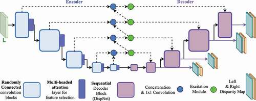
The proposed disparity estimation model follows that of an encoder-decoder structure and takes a single image as input. The encoder is a randomly connected fully convolutional neural network. It comprises of convolutional blocks that perform down-sampling of the input data and the decoder part performs up-sampling of the encoder feature maps to generate the left and right disparity maps hierarchically. Furthermore, we introduce skip connections with learn-able weights for improving the expressive power of the encoder. The overall architecture is shown in Figure 1. For training, we experiment with the loss function introduced in Godard et al. (2017) as our base loss function and propose a multi-scale adversarial image generation loss function.

Figure 1. The proposed encoder-decoder architecture. The solid and the dotted lines denote forward propagation and skip connections, respectively. The purple lines signify the output left and right disparity maps generated at 4 scales, each increasing hierarchically with a scale factor of 2.

3.1. Monocular depth estimation model

Randomly Connected Encoder: The encoder is initiated with a random graph, which is generated once in the beginning and subsequently converted to a directed acyclic graph (DAG). We modify Xie et al. (2019) to enable development of randomly connected encoder-decoder architectures for depth estimation. To define a randomly connected encoder-decoder architecture, we first divide the network into blocks as shown in Figure 1. This allows down-sampling to take place and provides more control on the size of the feature maps produced. Each block comprises its own random connections with $n$ number of nodes (i.e. operations) within it. The nodes within this graph are then mapped to their respective operations. The operations in the encoder layer are defined by a single convolution layer of a user-defined filter size, followed by normalisation and activation. The activation operation we use is eLU (Clevert et al. 2016). The process of random graph generation as illustrated in Figure 2 is the following:

• Step $a$ – Generate a list of $n$ nodes in a block and two fixed nodes, namely, an input and an output node. The two fixed nodes are placed in addition to the $n$ nodes within the block to allow inflow and outflow of feature maps;

• Step $b$ – Using the WS algorithm, randomly connect the nodes in the block;

• Step $c$ – Convert the nodes in the block to their respective operations;

• Step $d$ – On the aggregated feature maps from the output node, utilise multi-head self-attention for feature selection;

Figure 2. The process of generating a randomly connected deep-learning architecture. The red and the grey nodes are the input and the output nodes of the block, respectively. The black nodes are the convolution operations. The purple module is a multi-head self-attention module.

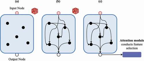
Once these blocks have been initiated, they are simply used as modules in the overall architecture as shown in Figure 1. In all cases, if there are more than one connections as input into a node, then the incoming feature maps are aggregated via a weighted sum with learn-able weights and then fed into their respective operations. If the output is to be sent to multiple nodes, then copies are made and sent. Since the feature maps are randomly connected, there is potentially misalignment between them when aggregated. Hence, we augment this backbone by using a multi-head, self-attention mechanism (Vaswani et al. 2017) at each encoder block. In particular, we use efficient attention with linear complexity as described in Shen et al. (2021). These attention mechanisms enable convolution layers to focus on key aspects via knowledge distillation by learning what to pay attention to. This is also vital for the skip connections, where this feature map misalignment can lead to poor localisation of features for disparity generation.

Furthermore, to generate connections between nodes, a seed is used to initialise a pseudo-random number generator. The pseudo-random number generator is used to generate up to $k$ pairs of random numbers for each node. $k$ is the maximum number of nearest neighbour nodes each node can connect to, and these pairs define the index of the other nodes that the candidate node will connect to. The process of graph generation, as shown in Figure 2, occurs in steps $a$ and $b$, which are highly susceptible to the random seeds selected, for initialising this pseudo-random generator. If only one seed value is selected (i.e. a global seed), then a single graph will be generated, which will be copied in every random block in step $d$. A global seed will initialise the same set of random number pairs every time, which will constrain the search space of connections. Another contribution of our work is the ‘cascaded random search’ process, which generates a large exploration space for connections. We modify the method in Xie et al. (2019) by introducing multiple seeds by multiplying the global seed with a multiplier, which in our case is the block number assigned sequentially. This allows each random block to have its own unique random seed. For example, if the global seed is 2, then for the model in Figure 1 and the first encoder block, the seed is 4 (i.e. 2 x 2, global seed value $\times$ layer number), for the second encoder block, the seed is 6 (2x3), for the third encoder block, the seed is 8 (2x4) and so on. This allows divergent graphs with unique random connections to be formed at each random cell enabling the exploration space to be large. We term this process ‘cascaded random search’. The multiplier can be any set of arbitrary numbers such that upon multiplying with the global seed value, a new seed value is generated for each block.

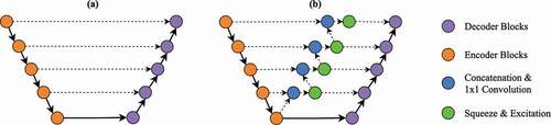
Learn-able Skip Connections: For the decoder to produce sharp disparity maps, it requires strong spatial and semantic features. In our case, semantic features are deep relationships hidden in surgical scenes, such as different tissue types and objects. This is typically stored in the channels of the feature maps. Spatial features help in localising boundary information, and this is fed to the decoder via skip connections as shown in Figure 3a. However, not much attention is given to semantic features. Zhou et al. (2018) showed that greater semantic feature representations are developed deeper through the network. For this reason, they created a densely connected U-Net, where every encoder layer feature map is connected to every ascending decoder layer. However, this explodes the parameter count and substantially increases training and inference times. Conversely, we take a more efficient approach to preserving these semantic features. Instead of densely connecting each encoder feature map, we concatenate the previous feature map with the adjacent one and perform 1 × 1 convolution for weighted compression. This prevents the parameter explosion. This is followed by squeeze and excitation modules (Hu et al. 2018), which individually weights these channels in importance (i.e. channel-wise attention) for the following convolution layer in the decoder. These weighted semantic features are then passed on to every ascending layers hierarchically. Allowing the model to maintain semantic features throughout each layer and to enable weighted aggregation of them for feature selection as shown in Figure 3b.

Figure 3. Showing the proposed learn-able skip connections methodology. $a$ is the network topology of a standard U-Net and $b$ is the proposed new network topology. Solid lines and dotted lines denote forward propagation and skip connections, respectively.

Decoder: Our decoder advances the architecture design proposed in Mayer et al. (2016). Unlike dispnet, which uses Mayer et al. (2016) interpolation for up-scaling the feature maps in the decoder, we utilise the Pixel Shuffle operation (Shi et al. 2016) followed by a convolution layer (filter size 3 × 3). As stated above, semantic features are usually overlooked and interpolation up-scales feature maps by linearly interpolating the spatial features. Instead, we reshuffle the deep channel feature maps to convert them into new spatial pixels and perform convolution for inferring these semantically up-sampled features into disparities. Figure 1 shows the final proposed model architecture, with all the components together where the encoder is randomly connected and the decoder is sequential as defined above. We also experimented with other model variants such as a fully random architecture where both the encoder and decoder blocks comprise randomly connected graphs and a hybrid model, where the encoder layers are sequential (from Resnet18 model (He et al. 2015)) and the decoder layers comprise randomly connected blocks. In our experiments, the proposed model performed the best, as the sequential decoder does not suffer from feature map misalignment like the random ones, which results in blurry disparities.

3.2. Loss function formulation

Our model is trained in a self-supervised manner using stereo video sequences, without requiring any ground truth disparities, similar to Godard et al. (2017). Given the left stereo-rectified image $I_L^{GT}$, the model produces the predicted left and right disparity maps $D_L^{pred}$ and $D_R^{pred}$. Since the disparity map defines the displacement of pixels from one camera frame to its corresponding stereo frame, a warping function can be applied to these disparities and the opposite images to regenerate the corresponding stereo frames $I_R^{Pred}$ and $I_L^{Pred}$. The intuition is that the generation of one image from the other in a stereo pair enforces the network to learn some aspect of the 3D shape of the scene. Hence, even with monocular input, the network intrinsically learns to develop both disparity maps. The loss function thus focuses on the reconstruction error between the predicted and the original images, which is used as ground truth. Standard loss components, which have been used for self-supervised disparity regression, include the image reconstruction loss $L_{recon}$, the disparity smoothness loss $L_{smooth}$ and the left-right disparity consistency loss $L_{LRcons}$ (Godard et al. 2017) as shown below:

(1) $L_{ssim}={\delta }_1{L}_{recon}+{\delta }_2{L}_{smooth}+{\delta }_3{L}_{LRcons}$(1)

The above loss terms are performed on both the generated left and right images. As stated above, the image reconstruction loss is crucial for achieving high performance in self-supervised depth estimation methods. Godard et al. (2017) in particular uses the multi-scale structural similarity index (MS-SSIM) (Wang et al. 2004) jointly with a L1 loss term as their $L_{recon}$. In our framework, since our model outputs disparity maps at four different scales, the MS-SSIM loss enables the model to hone the disparity output gradually as size increases. Additionally, it enables the reduction of artefacts being formed at the final output (at the largest scale).

Adversarial loss based on generative adversarial networks (GANs) have been employed for depth estimation for computing the photometric error (Pilzer et al. 2018)(Aleotti et al. 2018). To compute this loss, a generator $G$ and a discriminator $D$ is required. $G$ is the proposed model that generates the disparity maps and thereby the predicted images via warping. $D$ is a binary classifier that differentiates between ground truth images and the predicted images. The aim is to train $G$ and $D$ both to the point that $D$ can no longer differentiate between ground truth and the predicted images generated by $G$. This formulation does not account for the multi-scale penalty. The multi-scale penalty is vital, since standard adversarial losses tend not to specifically penalise for artefacts in the synthesised image, i.e. on the border regions or on the edges of objects where the depths are always not sharp enough to generate realistic warp colours. Adversarial loss alone fails to tackle this issue. In this work, in addition to MS-SSIM for $L_{recon}$, we propose a novel loss function based on multi-scale adversarial learning and perceptual loss. Our loss function allows for penalising poor quality generations at their respective scales. The naive approach to achieving this would involve having a discriminator $D$ dedicated to each scale. However, this would increase computation time and memory, requiring five networks being trained in parallel ($G$ and 4 $D$s, one for each scale). This also has the high risk of loss explosion, leading to $G$ potentially not converging or in some cases diverging. Instead, we define one $D$ network inspired by Karnewar and Wang (2020), and unlike other methods, where $D$ is some arbitrary sequential convolutional network; in our work, $D$ is similar to the specification of the $G$ encoder. 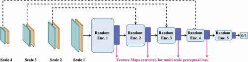Furthermore, we concatenate the output at each scale with the intermediate layers of $D$, enabling each block to learn features dedicated for the input at its respective scale as illustrated in Figure 4.

Figure 4. Discriminator model. The solid black lines and the dotted lines denote forward propagation and skip connections, respectively. The skip connection inputs are concatenated with the forward propagating feature map prior to being processed by the next layer. The pink lines show the extraction of multi-scale feature maps.

The multi-scale GANs loss for both $G$ and $D$ we experiment with is least squares GANs loss (Mao et al. 2017) (though any other type of GANs loss can be used):

(2) $L_{adv}^D=\frac{1}{2}[(D(I^{GT})-1{)}^2]+[(D(G(I_L^{GT})){)}^2]$(2)

(3) $L_{adv}^G=\frac{1}{2}[(D(G(I_L^{GT})))-1{)}^2]$(3)

$D$ takes both the left and right images concatenated as input. $I$ is the list of concatenated images for each of the four scales. The largest scale is parsed in via forward propagation, where the subsequent scales are concatenated with the forward propagating feature map before being fed into their respective intermediate layers. This enables the intermediate layers to learn the features dedicated for differentiating real and fake data for that particular scale. Furthermore, Johnson et al. (2016) showed that high fidelity images can be constructed through perceptual loss functions. It encourages the predicted outputs to have similar feature representations as the ground truth using features extracted from pre-trained networks. We adopt this to a multi scale feature reconstruction loss by directly using our multi-scale discriminator as the feature extractor. This allows the feature matching to occur at each scale. The discriminator block with large receptive fields, i.e. $Enc1$ learns global features such that $G$ generates globally consistent outputs at the largest scale, while the blocks with smaller receptive fields, i.e. $Enc3$ learn local features, ensuring $G$ produces sharper details. This combination enables $G$ to generate outputs with less artefacts, especially in low-textured scenes prevalent in MIS data. We experiment with the feature reconstruction loss ($L_{feat}$), as displayed in the below equation:

(4) $L_{feat}={\mathrm{\Sigma }}_{n=1}^{N=4}||D_n(D_{n-1},I_n^{pred})-D_n(D_{n-1},I_n^{GT})|{|}_1$(4)

Where $n$ is the scale and for the discriminator it is the respective layer number too. Like above, $I$ are the list of images at each of the four scales. The final loss function is:

(5) $\begin{array}{rl}& L_{final}={\delta }_1{L}_{recon}+{\delta }_2{L}_{smooth}+\\ & {\delta }_3{L}_{LRcons}+{\delta }_4{L}_{adv}^G+{\delta }_5{L}_{feat}\end{array}$(5)

4. Experimental results and discussion

4.1. Implementation details

The square filter sizes of the convolution operations in the encoder blocks sequentially are [7,5,3,3,3]. The number of blocks and the filter sizes are consistent with the model in Godard et al. (2017) to allow fair comparison. With the exception, standard (Godard et al. 2017) model comprises seven layers of the encoder, whereas ours is smaller comprising of five layers. The proposed model is trained to for 200 epochs. The input and output image resolutions are 256 × 512. The loss weightings in Equation (5)(5) $\begin{array}{rl}& L_{final}={\delta }_1{L}_{recon}+{\delta }_2{L}_{smooth}+\\ & {\delta }_3{L}_{LRcons}+{\delta }_4{L}_{adv}^G+{\delta }_5{L}_{feat}\end{array}$(5) are as follows: ${\delta }_1$, ${\delta }_2$, ${\delta }_3$, ${\delta }_4$ and ${\delta }_5$ are 0.85, 1.0, 1.0, 1.0 and 0.05, respectively. For the graph generation algorithm WS, the maximum k nearest neighbours for node selection was 4, the total number of nodes $n$ was 5, and the probability of rewiring an edge was 0.75. For training with $L_{feat}$, the loss calculation starts after 10 epochs to give the discriminator enough time to become a good classifier. Both the proposed disparity estimation model and the discriminator are trained with the Adam optimiser with a learning rate of 0.0001. The model was trained on MIS data from the Hamlyn database (Giannarou et al. 2013), where 34,240 frames were used for training and 7,191 for testing. The models pre-trained on the Hamlyn data were later fine-tuned on SCARED (Giannarou et al. 2013) for further evaluation. The models were trained on an Nvidia Tesla T4. The training computation time for the proposed model trained with $L_{final}$ is 3 GPU days, whereas training with $L_{ssim}$ is 1.5 GPU days.

4.2. Performance evaluation

For SCARED data, we use the same evaluation metrics as defined in their paper (Allan et al. 2021), which is the mean absolute depth error (in mm) on test datasets 1 and 2. We show comparison with other self-supervised methods submitted to this challenge for both the test datasets presented in the challenge. For Hamlyn data, due to lack of ground truth depth, we compare the structural similarity index (SSIM) between the ground truth and the predicted images followed by warping, same as Ye et al. (2017), which is used for comparison. In both cases, the original methods proposed by the authors were stereo models, whereas our method is a monocular model. Due to lack of availability of monocular models in surgical data, we continue with comparison to stereo models on these benchmarks. Furthermore, the performance of the proposed method is qualitatively compared on both the datasets in Figure 5. We also re-train the state-of-the-art monocular models trained via stereo images, i.e. Godard et al. (2017) and Pilzer et al. (2018) on the Hamlyn dataset to enable comparison with monocular models. We show qualitative comparison of the monocular models on Hamlyn in Figure 6.

Figure 5. Depth maps generated by the proposed model on the SCARED and Hamlyn test splits shown in rows $A$ and $B$, respectively. Inclusion of $LS$ signifies presence of learn-able skip connections and $noLS$ without. All models were trained with the standard $L_{ssim}$ loss (Equation 1(1) $L_{ssim}={\delta }_1{L}_{recon}+{\delta }_2{L}_{smooth}+{\delta }_3{L}_{LRcons}$(1) ) unless $L_{Final}$ is specified, which signifies training with the proposed loss function (Equation 5(5) $\begin{array}{rl}& L_{final}={\delta }_1{L}_{recon}+{\delta }_2{L}_{smooth}+\\ & {\delta }_3{L}_{LRcons}+{\delta }_4{L}_{adv}^G+{\delta }_5{L}_{feat}\end{array}$(5) ). The colour bar displays the depth range in mm.

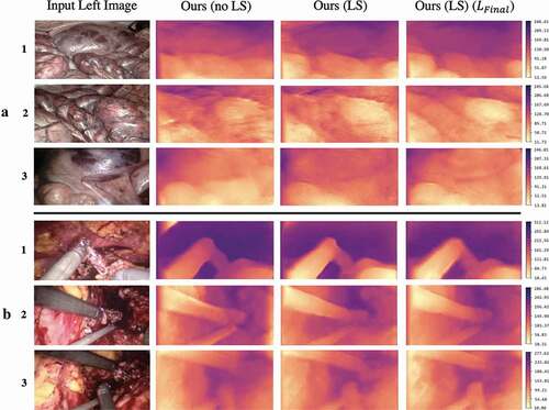
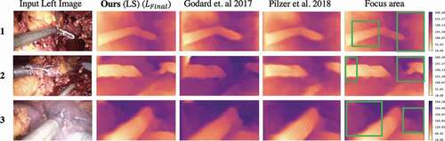
Figure 6. Comparison of depth maps generated by our model with Godard et al. (2017) and Pilzer et al. (2018) on the Hamlyn test split. The last column re-displays the depth produced by our proposed method (column 2), with the green boxes highlighting the key areas where more details are visible in our depth maps. The colour bar displays the depth range in mm.

As it can be observed from Figure 5, in both the datasets, the proposed model variant with learnable-skip connections (LS) (column 3) generates far less artefacts than the model without (no LS) (column 2). This is further visible on the depth maps in row $B.1$, where the top left corner of the depth map generated by our model with no LS has a more prominent artefact than the variant with LS. Furthermore, LS also enables development of sharper depth maps, more consistent with the shapes appearing in the scene. This can be observed when comparing both the samples in row $A$, where the LS variant generates more consistent contours around boundaries of the soft tissues. Training with $L_{Final}$ further enhances the results by removal of artefacts around edges and boundaries of tools and soft tissues. This is visible in all the depth maps generated by the final proposed model (column 4) for all the samples. We believe the multi-scale adversarial loss is capable of penalising for these corner artefacts that are usually tricky for MS-SSIM whilst generating sharp, yet smooth depth maps. Row $A.2$, is particularly a tough challenge for deep learning models due to the reflections present in the scene. As it can be observed, both model variants with and without LS fail to generate sharp depth maps. However, the model variant trained with $L_{Final}$ resolves a high fidelity depth robust to such effects, showing the importance of multi-scale deep feature losses for photometric error calculation. The superiority of our model and loss function is further displayed in Figure 6, where it is compared against 2 state-of-the-art monodepth models. The final column ’Focus area’ highlights in green boxes where the generated depth maps by our model achieves finer details than the competition exhibiting the importance of both the architecture design and multi-scale penalty for adversarial learning, in generating such sharper details. One can observe that our model generates sharper depth for anatomical structures present around the tools, which is a challenge for the other two methods. Moreover, the image in row 3 includes smoke, which occludes some of the soft anatomical structures in the background. As it can be deduced, our model uncovers depth for such regions too. Lastly, in row 2, our method generates less artefacts in corner regions of the image, as the multi-scale deep feature loss enforces the model to maintain global and local consistency.

The proposed model is also quantitatively validated and compared to the latest surgical depth estimation benchmark on the SCARED dataset in Tables 1 and 2. We compare with the self-supervised submissions for a fair comparison albeit, the competing methods are stereo models. Overall, the best performing model in test dataset 1 is ours, and despite being monocular, our method is comparable to the other stereo models in test dataset 2. We believe this is because both the stereo methods ’KeXue Fu’ and ’Xiaohong Li’ (Allan et al. 2021) follow the loss function and model introduced by Godard et al. (2017) and Pilzer et al. (2018) though adapted for stereo. As shown in Figure 6, they are both prone to generating artefacts, especially near edges and boundaries of soft tissue structures. This is due to both the potential sub-optimal model and the loss function’s inability to penalise for high-order inconsistencies in the warped images. This is what we try to address in this work, with a loss function with stronger emphasis on image reconstruction not only via MS-SSIM but also via efficient multi-scale discriminator and deep feature perceptual losses. The proposed model enforces local and global consistency even for monocular depth estimation, while providing a more exploratory approach to model design (randomly connected encoder and learn-able skip connections). Furthermore, from the ablation study, one can observe that the performance of all the model variants is comparable with the other stereo competitors. In particular, our proposed method with no learn-able skip connections (no LS) trained on the standard $L_{ssim}$ loss function is comparable to the other stereo models despite being monocular. The only novel component in this variant is the random connections, which further exemplifies the power of innovative topology for neural architecture designs. The addition of learn-able skip connections further improves on these results, due to the extra attention paid to the deep semantic features.

Table 1. Showing the mean absolute depth error in mm for test dataset 1 from SCARED. The compared methods are the self-supervised methods submitted to this challenge. (M) signifies Monodepth method and (S) Stereodepth. The presence of $L$ denotes the type of loss function used for training, and presence of (no LS) implies no learn-able skip connections were used in the model. Best results are highlighted in bold

Method	Keyframe 1	Keyframe 2	Keyframe 3	Keyframe 4	Keyframe 5	Average
Ours $L_{final}$ (M)	34.18 $\pm$ 0.071	27.01 $\pm$ 0.096	14.82 $\pm$ 0.063	13.42 $\pm$ 0.055	12.89 $\pm$ 0.067	20.46
Ours $L_{ssim}$ (M)	33.21 $\pm$ 0.069	26.73 $\pm$ 0.099	15.47 $\pm$ 0.066	15.13 $\pm$ 0.058	13.01 $\pm$ 0.066	20.71
Ours $L_{ssim}$ (no LS) (M)	35.02 $\pm$ 0.074	28.10 $\pm$ 0.091	16.89 $\pm$ 0.061	17.76 $\pm$ 0.061	13.26 $\pm$ 0.068	22.206
KeXue Fu (S)	30.49	18.32	19.73	19.30	16.86	20.94
Xiaohong Li (S)	34.42	20.66	17.84	27.92	13.00	22.77

Table 2. Showing the mean absolute depth error in mm for test dataset 2 from SCARED. The compared methods are the self-supervised methods submitted to this challenge. Where (M) signifies Monodepth method and (S) Stereodepth. The presence of $L$ denotes the type of loss function used for training, and presence of (no LS) implies no Learn-able skip connections were used in the model. Best results are highlighted in bold

Method	Keyframe 1	Keyframe 2	Keyframe 3	Keyframe 4	Keyframe 5	Average
Ours $L_{final}$ (M)	29.00 $\pm$ 0.061	25.81 $\pm$ 0.092	18.72 $\pm$ 0.064	8.90 $\pm$ 0.070	10.12 $\pm$ 0.044	18.51
Ours $L_{ssim}$ (M)	27.69 $\pm$ 0.059	26.17 $\pm$ 0.091	20.14 $\pm$ 0.061	9.11 $\pm$ 0.068	11.79 $\pm$ 0.054	18.98
Ours $L_{ssim}$ (no LS) (M)	28.25 $\pm$ 0.066	27.36 $\pm$ 0.088	22.83 $\pm$ 0.065	11.69 $\pm$ 0.073	13.51 $\pm$ 0.055	20.73
KeXue Fu (S)	23.71	15.46	26.43	9.60	10.92	17.22
Xiaohong Li (S)	24.58	16.80	29.92	11.37	19.93	20.52

Considering Table 3, our solution supersedes monocular and stereo depth estimation methods, including Ye et al.’s (2017) stereo model. Despite our model comprising of a smaller memory footprint with significantly less parameters for training, it still outperforms the others. This shows the importance of innovative architecture design, which does not require over-parameterised models. The above results verify that the convolution operation itself is very powerful, such that even a randomly connected network with enough convolution operations is capable of successfully learning a task. This suggests that more focus needs to go on architecture design for optimising monocular depth.

Table 3. SSIM index on the reconstructed images generated via the estimated disparity maps on the Hamlyn test dataset. Higher value indicates better performance. Where (M) signifies Monodepth method and (S) Stereodepth. The M in parameter count signifies a million parameters. Methods $A$,$B$,$C$,$D$ and $E$ are Geiger et al. (2010), Yamaguchi et al. (2014), Ye et al. (2017), Godard et al. (2017) and Pilzer et al. (2018), respectively

Method	A (S)	B (S)	C (S)	D (M)	E (S)	Ours (M)
Mean SSIM	0.473	0.547	0.604 $\pm$ 0.066	0.611 $\pm$ 0.076	0.633 $\pm$ 0.079	0.672 $\pm$ 0.080
Parameter count	–	–	32 M	31 M	31 M	22 M

We believe the proposed methodology guides researches in understanding how to improve monocular depth estimation without reliance on capturing arduous ground truth. To that extent, we can further improve the proposed method for clinical deployment. In clinical applications, depth error should be typically in the range of sub-mm accuracy. Our method currently does not achieve this accuracy. However, it is still superior to state-of-the-art methods for monocular surgical scene reconstruction. In our future work, we aim to improve the performance of our model by experimenting with better architecture exploration strategies, which is key for training robust monocular models. More specifically, we will test more sophisticated architecture search strategies that optimise the random connections, such as population-based search (Geiger et al. 2010) and further pruning of extra unnecessary parameters and connections (Tanaka et al. 2020). This will provide a better search and selection criteria in place of random connections and self-attention.

5. Conclusion

Both the neural architecture and the loss function play a vital role in the performance of a neural network. In this work, we showed that the biggest factor in optimising monocular depth is the design of the neural network architecture itself and the loss function’s capability of computing high-order multi-scale image reconstruction metrics. We proposed the first method to generate randomly connected encoder-decoder networks and a new U-net topology for exploiting hidden semantic features. Our results verify that even a randomly connected network with standard convolution operations but innovative inter-connections can learn the task well. Additionally, we showed that multi-scale penalty in loss functions is vital for generating finer details. We believe that our study will aid in further research of neural network architecture design and shift from the standard U-net and manual trial and error based approaches to more automated design methods. Our future work will entail experimenting with more loss terms and exploring more inventive methods of conducting search in the connections space to see how other variations of the network impact the results.

Acknowledgments

Dr Giannarou and Mr Tukra are supported by the Royal Society (UF140290 and RGF80084) and the NIHR Imperial Biomedical Research Centre (BRC).

Disclosure statement

No potential conflict of interest was reported by the author(s).

Additional information

Funding

This work was supported by the Royal Society [UF140290 and RGF80084] and the NIHR Imperial Biomedical Research Centre.

Notes on contributors

Samyakh Tukra

Samyakh Tukra is Ph.D. candidate in the Hamlyn Centre for Robotic Surgery at Imperial College London, United Kingdom. He received an M.Eng. in Medical Engineering at Cardiff University in 2017, and an MSc. in Human and Biological Robotics at Imperial College London in 2018. His research focus is in Computer Vision, Machine/Deep Learning, Reinforcement Learning and AutoML algorithms.

Stamatia Giannarou

Stamatia Giannarou received a PhD in object recognition from the Department of Electrical and Electronic Engineering, Imperial College London, UK. She is a Royal Society University Research Fellow at the Hamlyn Centre for Robotic Surgery and a lecturer in Surgical Cancer Technology and Imaging at the Department of Surgery and Cancer, Imperial College London, UK. Her research focuses on enhanced surgical vision for navigation during minimally invasive and robot-assisted operations.

References

- Aleotti F, Tosi F, Poggi M, Mattoccia S. 2018. Generative adversarial networks for unsupervised monocular depth prediction. In: Proceedings of the European Conference on Computer Vision (ECCV) Workshops; September.
- Allan M, McLeod AJ, Wang CC, Rosenthal J, Hu Z, Gard N, Eisert P, Fu KX, Zeffiro T, Xia W, et al. 2021. Stereo correspondence and reconstruction of endoscopic data challenge. CoRR. abs/2101.01133. Available from: https://arxiv.org/abs/2101.01133
- Cao ZW Y, Shen C. 2018. Estimating depth from monocular images as classification using deep fully convolutional residual networks. p. 3174–3182. Available from: https://ieeexplore.ieee.org/document/8010878/authors#authors
- Clevert D, Unterthiner T, Hochreiter S. 2016. Fast and accurate deep network learning by exponential linear units (elus). In: Bengio Y, LeCun Y, editors. 4th International Conference on Learning Representations, ICLR 2016; 2016 May 2-4; San Juan, Puerto Rico: Conference Track Proceedings. Available from: http://arxiv.org/abs/1511.07289
- Eigen D, Puhrsch C, Fergus R. 2014. Depth map prediction from a single image using a multi-scale deep network. In: Ghahramani Z, Welling M, Cortes C, Lawrence ND, Weinberger KQ, editors. Advances in neural information processing systems 27; Curran Associates, Inc, Palais des Congrès de Montréal, Montréal CANADA.; p. 2366–2374. Available from: http://papers.nips.cc/paper/5539-depth-map-prediction-from-a-single-image-using-a-multi-scale-deep-network.pdf.
- Fu H, Gong M, Wang C, Batmanghelich K, Tao D. 2018. Deep ordinal regression network for monocular depth estimation. IEEE Conference on Computer Vision and Pattern Recognition (CVPR). 2018(6):2002–2011.
- Garg R, Kumar BV, Carneiro G, Reid I. 2016. Unsupervised CNN for single view depth estimation: geometry to the rescue. In: European Conference on Computer Vision; Amsterdam, the Netherlands,: Springer; p. 740–756.
- Geiger A, Roser M, Urtasun R. 2010. Efficient large-scale stereo matching. ACCV. Berlin, Heidelberg: Springer
- Giannarou S, Visentini-Scarzanella M, Yang GZ. Probabilistic tracking of affine-invariant anisotropic regions. IEEE Trans Pattern Anal Mach Intell. 2013. Jan; 35(1):130–43. doi:https://doi.org/10.1109/TPAMI.2012.81. PMID: 22450819.
- Godard C, Mac Aodha O, Brostow GJ. 2017. Unsupervised monocular depth estimation with left-right consistency. In: IEEE Conference on Computer Vision and Pattern Recognition (CVPR), Honolulu, Hawaii.
- Godard, Clément, Oisin Mac Aodha and Gabriel J. Brostow. “Digging Into Self-Supervised Monocular Depth Estimation.” 2019 IEEE/CVF International Conference on Computer Vision (ICCV) (2019): 3827–3837.
- He K, Zhang X, Ren S, Sun J 2015. Deep residual learning for image recognition. Computer Vision and Pattern Recognition (CVPR). abs/1512.03385. Available from: http://arxiv.org/abs/1512.03385
- Hu J, Shen L, Sun G. 2018. Squeeze-and-excitation networks. In: Proceedings of the IEEE Conference on Computer Vision and Pattern Recognition (CVPR), Salt Lake City, Utah; June.
- Huang G, Liu Z, van der Maaten L, Weinberger KQ. 2017. Densely connected convolutional networks. In: Proceedings of the IEEE Conference on Computer Vision and Pattern Recognition, Honolulu, Hawaii.
- Jaderberg M, Simonyan K, Zisserman A, Kavukcuoglu K. 2015. Spatial transformer networks. In: Cortes C, Lawrence ND, Lee DD, Sugiyama M, Garnett R, editors. Advances in neural information processing systems 28; Curran Associates, Inc.; p. 2017–2025. Available from: http://papers.nips.cc/paper/5854-spatial-transformer-networks.pdf.
- Johnson J, Alahi A, Fei-Fei L 2016. Perceptual losses for real-time style transfer and super-resolution. In: European Conference on Computer Vision.
- Karnewar A, Wang O 2020. MSG-GAN: multi-scale gradients for generative adversarial networks. In: 2020 IEEE/CVF Conference on Computer Vision and Pattern Recognition, CVPR 2020; 2020 Jun 13; Seattle, WA, USA: IEEE; p. 7796–7805. Available from: https://doi.org/10.1109/CVPR42600.2020.00782.
- Liang, Zhengfa, Yiliu Feng, Yulan Guo, Hengzhu Liu, Wei Chen, Linbo Qiao, Li Zhou and Jianfeng Zhang. “Learning for Disparity Estimation Through Feature Constancy.” 2018 IEEE/CVF Conference on Computer Vision and Pattern Recognition (2018): 2811–2820.
- Mao X, Li Q, Xie H, Lau RYK, Wang Z, Smolley SP. 2017. Least squares generative adversarial networks. 2017 IEEE International Conference on Computer Vision (ICCV), Venice, Italy; p. 2813–2821.
- Mayer N, Ilg E, Häusser P, Fischer P, Cremers D, Dosovitskiy A, Brox T. 2016. A large dataset to train convolutional networks for disparity, optical flow, and scene flow estimation. In: 2016 IEEE Conference on Computer Vision and Pattern Recognition, CVPR 2016; 2016 Jun 27-30; Las Vegas, NV, USA: IEEE Computer Society; p. 4040–4048. Available from: https://doi.org/10.1109/CVPR.2016.438.
- Pilzer, Andrea, Dan Xu, Mihai Marian Puscas, Elisa Ricci and N. Sebe. 2018. “Unsupervised Adversarial Depth Estimation Using Cycled Generative Networks.” 2018 International Conference on 3D Vision (3DV) : 587–595.
- Poggi M, Tosi F, Mattoccia S 2018. Learning monocular depth estimation with unsupervised trinocular assumptions. 2018 International Conference on 3D Vision (3DV):324–333.
- Shen Z, Zhang M, Zhao H, Yi S, Li H. 2021. Efficient attention: attention with linear complexities. WACV.
- Shi W, Caballero J, Huszar F, Totz J, Aitken AP, Bishop R, Rueckert D, Wang Z. 2016. Real-time single image and video super-resolution using an efficient sub-pixel convolutional neural network. In: CVPR; IEEE Computer Society, Caesars Palace in Las Vegas, Nevada; p. 1874–1883. Available from: http://dblp.uni-trier.de/db/conf/cvpr/cvpr2016.html#ShiCHTABRW16
- Tanaka H, Kunin D, Yamins DL, Ganguli S 2020. Pruning neural networks without any data by iteratively conserving synaptic flow. In: Larochelle H, Ranzato M, Hadsell R, Balcan MF, Lin H, editors. Advances in Neural Information Processing Systems; vol. 33. Curran Associates, Inc.; p. 6377–6389. Available from: https://proceedings.neurips.cc/paper/2020/file/46a4378f835dc8040c8057beb6a2da52-Paper.pdf
- Vaswani A, Shazeer N, Parmar N, Uszkoreit J, Jones L, Gomez AN, Kaiser L, Polosukhin I 2017. Attention is all you need. In: Guyon I, Luxburg UV, Bengio S, Wallach H, Fergus R, Vishwanathan S, Garnett R, editors. Advances in Neural Information Processing Systems; vol. 30. Long Beach Convention Center, Long Beach: Curran Associates, Inc.; Available from: https://proceedings.neurips.cc/paper/2017/file/3f5ee243547dee91fbd053c1c4a845aa-Paper.pdf
- Wang Z, Bovik AC, Sheikh HR, Simoncelli EP. 2004. Image quality assessment: from error visibility to structural similarity. IEEE Trans Image Process. 13(4):600–612. Available from. doi:https://doi.org/10.1109/TIP.2003.819861.
- Watson J, Firman M, Brostow GJ, Turmukhambetov D 2019. Self-supervised monocular depth hints. In: The International Conference on Computer Vision (ICCV); October.
- Watts D, Strogatz S. 1998. Collective dynamics of ’small-world’ networks. Nature. 393(6684):440–442. doi:https://doi.org/10.1038/30918.
- Xie J, Girshick RB, Farhadi A 2016. Deep3d: fully automatic 2d-to-3d video conversion with deep convolutional neural networks. In: European Conf. Amsterdam, The Netherlands: Computer Vision (ECCV).
- Xie S, Kirillov A, Girshick RB, He K 2019. Exploring randomly wired neural networks for image recognition. 2019 IEEE/CVF International Conference on Computer Vision (ICCV); p. 1284–1293.
- Yamaguchi K, McAllester DA, Urtasun R 2014. Efficient joint segmentation, occlusion labeling, stereo and flow estimation. In: ECCV, Zurich, Switzerland.
- Ye M, Johns E, Handa A, Zhang L, Pratt P, Yang G 2017. Self-supervised siamese learning on stereo image pairs for depth estimation in robotic surgery. ArXiv. abs/1705.08260.
- Yosinski J, Clune J, Bengio Y, Lipson H 2014. How transferable are features in deep neural networks? In: Ghahramani Z, Welling M, Cortes C, Lawrence N, Weinberger KQ, editors. Advances in Neural Information Processing Systems; vol. 27. Curran Associates, Inc.; Available from: https://proceedings.neurips.cc/paper/2014/file/375c71349b295fbe2dcdca9206f20a06-Paper.pdf
- Zhou, Zongwei, Md Mahfuzur Rahman Siddiquee, Nima Tajbakhsh and Jianming Liang. “UNet++: A Nested U-Net Architecture for Medical Image Segmentation.” Deep Learning in Medical Image Analysis and Multimodal Learning for Clinical Decision Support : 4th International Workshop, DLMIA 2018, and 8th International Workshop, ML-CDS 2018, held in conjunction with MICCAI 2018, Granada, Spain, 11045 (2018): 3–11.