Social vulnerability and local economic outcomes during the COVID-19 pandemic

ABSTRACT

This paper investigates factors associated with disparities in the exposure of US counties to the initial COVID-19 economic shock in early 2020 and their disparate economic recovery paths during the pandemic. We focus on three alternative composite measures of social vulnerability to disasters: the Centers for Disease Control and Prevention’s Social Vulnerability Index, the University of South Carolina’s Social Vulnerability Index and the Census Bureau’s Community Resilience Estimate. Empirical evidence under the conventional ‘global’ regression approach supports a cross-sectional correlation between the social vulnerability indices and local economic outcomes during the recovery phase, although the results are equivocal for characterising uneven local economic downturns triggered by the pandemic. Economic outcomes were dominated by other local characteristics, including population density, the share of hospitality employment, government policy measures and unobservable factors. In addition to validating the empirical relevance of the social vulnerability indices in the context of the COVID-19 pandemic, a geographically and temporally weighted autoregressive model offers insights into both disparate and clustering patterns across broad regions in the role of inherent sociodemographic attributes for characterising local economic dynamics over time.

KEYWORDS:

• COVID-19 pandemic
• social vulnerability
• spatial dependence
• spatial heterogeneity
• geographically and temporally weighted autoregressive model

1. INTRODUCTION

The United States fell into a deep recession in early 2020 as COVID-19 outbreaks led to a nationwide lockdown. By mid-2022 the US’s overall economy had recovered almost all the jobs lost in the recession. Yet local economic performance was uneven across the nation, some communities had surpassed their historical baselines while others had continued to lag behind. What contributed to the uneven nature of the downturn during the onset of the pandemic and subsequent economic recovery across the nation?

Recent social science research has advanced the concepts of social vulnerability and community resilience to disruptive events, particularly natural and human-caused disasters like pandemics. Social vulnerability broadly refers to the potential adverse effects of disasters on communities and community resilience reflects the ability to withstand such disruptions and recover rapidly (Bakkensen et al., 2017). Given more frequent and intensive disaster events due to climate change in recent years, these concepts have become guiding principles for strategic planning and management decisions among US government agencies, including the Federal Emergency Management Agency (FEMA) and the Centers for Disease Control and Prevention (CDC). The abundant research on the role of inherent sociodemographic attributes for understanding community-level vulnerability or resilience to disasters (e.g., Bakkensen et al., 2017; Cutter et al., 2008; Fatemi et al., 2017) has motivated our study in the context of the COVID-19 pandemic.

Partly because of the definitional vagueness of the concepts of social vulnerability and resilience, there is no consensus on their measurements. Cutter et al. (2008) detail the conceptual linkages between these two concepts. Bergstrand et al. (2015) document disparities in the distribution of social vulnerability and resilience across US regions, while O’Brien et al. (2007) explain how different conceptualisations of vulnerability and resilience affect the ways research and policy decisions are carried out. These two interrelated interpretations represent complementary approaches to disaster issues. Nevertheless, the cornerstones of this line of research are typically single quantitative indicators that purport to be informative for community stakeholders and policymakers alike to better prepare for and respond to disaster events. Derakhshan et al. (2022) find little overlap among those measurements for many US communities defined by counties, while Cutter et al. (2014) find that their relationships vary across broad regions. From this perspective, we compare the results from some prominent measurements: the CDC’s Social Vulnerability Index (SVI) (Flanagan et al., 2011), the University of South Carolina Hazards and Vulnerability Research Institute’s Social Vulnerability Index (SoVI) (Cutter et al., 2014) and the Census Bureau’s Community Resilience Estimates (CRE).

Given the unprecedented nature of the COVID-19 pandemic it is interesting to review how well those popular disaster-oriented social indices explain the varying susceptibility of local economies to COVID-induced economic shocks and their performance in the context of subsequent recovery over time. To track changes in local economic conditions over time, we look at county-level employment, unemployment and an overall measure of economic activity, as suggested by Rose (2021).

Much of the literature on the impact of COVID-19 on the economy relies on a modelling approach to performing ex ante projections of initial economic losses and subsequent recovery paths (Kajitani et al., 2023; Mandel & Veetil, 2020; Walmsley et al., 2021). Ex post analyses of macroeconomic outcomes during the pandemic remain sparse. A major challenge for a formal analysis of the role of inherent sociodemographic characteristics in explaining disparate local economic outcomes arises from a variety of confounding factors that also shape the local economies. Notably, despite the federal government’s COVID-related policy recommendations, containment measures in the early months of the pandemic and subsequent support for recovery and public health, including school and workplace re-openings, mask mandates and vaccination campaigns, varied substantially across the nation’s 50 states. State governments’ responses to COVID-19 were likely to be contingent on political and social contexts. Disparities in people’s behaviour in response to government policies and interventions also underscore the importance of controlling for local-level heterogeneity other than social vulnerability in characterising the local economy throughout the pandemic.

The objective of this paper is to understand how US counties with diverse sociodemographic attributes were exposed to the initial COVID-19 economic shock in early 2020 and how they bounced back from the historic downturn. To this end, we empirically evaluate the validity of some prominent composite social indices in explaining key economic outcomes. Regional disparities in social vulnerability conditions are well documented in the literature (Cutter et al., 2014, 2016; Park & Xu, 2020). As such, some aspects of social vulnerability may explain economic outcomes in some counties or broad regions but not others. On the other hand, the economy of one county is interconnected with the economies of its neighbouring counties, especially in the wake of major disasters (Belasen & Polachek, 2009; Lee, 2021). Economic spillovers across local communities bring about spatial dependence in economic outcomes. In this study, we apply a geographically weighted autoregressive (GWAR) framework to account for both spatial heterogeneity and spatial dependence in modelling relationships across counties (Geniaux & Martinetti, 2018; Peng et al., 2020). To better understand how the role of social vulnerability also evolved over time since the onset of the pandemic, we further incorporate the temporal dimension of the spatial-oriented data into a geographically and temporally weighted autoregressive (GTWAR) model (Wu et al., 2014).

The rest of the paper is organised as follows. The next section describes our data and empirical models for analysing the role of social vulnerability in explaining exposure to COVID-19’s economic impacts in early 2020 and the subsequent recovery across US counties. The third section discusses model regression results, followed by conclusive remarks in the fourth section.

2. DATA AND METHOD

2.1. Local economic outcomes

This study focuses on the role of social vulnerability in explaining variations in local economic outcomes during the first wave of COVID-19 outbreaks among US communities and their subsequent recovery through the end of 2022. To characterise local economic conditions we employ county-level data. Local labour market conditions are measured alternatively by the employment level and the unemployment rate of each of the 3142 US counties and county equivalents. The data are sourced from the Bureau of Labor Statistics’ Local Area Unemployment Statistics (LAUS) programme. We apply the X-11 procedure to remove seasonal factors from the raw data.

Monthly data for measuring overall economic activity at the county level are not typically available. However, to monitor local economic recovery during the pandemic, the Department of Energy’s Argonne National Laboratory has developed the County Economic Impact Index (CEII) as a proxy for the gross regional output of a county (Smith et al., 2021). The CEII data are seasonally adjusted at the source.

Figure 1 shows the patterns of the county-level employment, unemployment and output data by decile between January 2020 and December 2022. For employment and output, the data are expressed relative to their January 2020 levels. The dotted lines represent the median values. The COVID-induced recession officially lasted for three months between February and April 2020. By April, a typical US county was down by roughly 10% in economic output and 12% in employment, while its unemployment rate surged to 11%. These median local economic impact measures seem less severe than the official nationwide figures that are adjusted for individual counties’ population sizes. Likewise, the plots show that the typical county’s three overall economic outcomes returned to the pre-pandemic levels within the first quarter of 2022, about one quarter earlier than what the national-level data suggest.

Figure 1. County-level employment, unemployment and output by decile.

Three line graphs plotting the relative levels of employment, unemployment and output from January 2020 to December 2022. The medians are surrounded by levels at every 10 percentiles above and below.

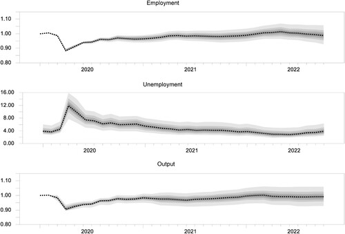
Overall, the plots in Figure 1 reveal remarkable disparities among US local economies over time. Local unemployment rates varied more widely during the nationwide recession than during the subsequent recovery phase. In fact the distributions of employment and output tended to widen over time after the nationwide recession ended in April. Employment among counties in the top 10 percentile was fully restored as early as January 2021, while employment among counties in the bottom 10 percentile still averaged roughly 10% behind the pre-pandemic level. Output as an aggregate measure of the economic activity tended to move in unison with employment but at a slower pace.

2.2. Social vulnerability indices

To explore factors that help explain disparities in local economic conditions during the pandemic, we focus on measures of social vulnerability. The interrelated concepts and measures of social vulnerability and community resilience have been the cornerstones for researchers, government planners and officials to facilitate emergency responses and resource allocations for individual communities subject to a broad range of disruptive events, from natural disasters to disease outbreaks. The most common methodology is the construction of a quantitative composite metric from constituent components capturing a multitude of inherent sociodemographic and institutional characteristics that potentially affect individual communities’ capacity to resist a disaster and recover from it. FEMA (2022) has provided a detailed review of those measurements and their methodologies, and Bakkensen et al. (2017) have evaluated them in the context of historical natural disasters in the southeastern United States.

Given our case study of the COVID-19 pandemic, we consider three social vulnerability indices: the SVI (Flanagan et al., 2011), SoVI (Cutter et al., 2014) and CRE (Willyard et al., 2022). Other popular measurements, such as the Baseline Resilience Indicators for Communities (BRIC) developed by Cutter et al. (2008, 2014) and FEMA’s Community Resilience Index (FEMA, 2022), are explicitly geared towards such natural disasters as storms and wildfires that cause physical damage. For instance, BRIC includes infrastructural and environmental determinants that are largely irrelevant to the COVID-19 pandemic.

On the contrary, the CDC developed its SVI explicitly for disease outbreaks, SoVI has long been a well-known measure of social vulnerability and thus can serve as a benchmark for comparison while the Census Bureau’s CRE is one of the newest indices. Willyard et al. (2022) discuss two key advantages of CRE over other indices. First, CRE’s data are more precise than other popular measures of social vulnerability or resilience that also rely on data from the American Community Survey (ACS) because it derives from microdata or person-level data instead of a geographic level. Other social vulnerability indicators reflect phenomena experienced by individuals, but they rely on public data that are available only at a community level instead of personal level. Second, instead of using ACS five-year data, CRE data are model-based estimates based on ACS one-year data that are not publicly available for counties or smaller entities. As a result, the CRE data are more timely for characterising areas that have experienced major changes.

Table 1 lists the constituent components of the three social indices, grouped into seven categories: demographic, economic, household composition, employment, transportation, health and communication. Both the overlapping nature of those composite measures and the differences in input variables are apparent. The CDC’s SVI is a composite index of the summed percentile rankings of 15 variables of census data. The SoVI is the outcome of a principal component analysis of 28 variables, the most among the three social indices. The Census Bureau’s CRE programme considers 10 characteristics of individuals or households as ‘risk factors’. For consistency in interpretation with the other two indices in this study, we collect the county-level CRE data for the rate of individuals with at least one of those 10 risk factors listed in Table 1. This ‘vulnerable’ population share ranges between 44% and 95% across counties, with a median of 67%.

Table 1. Comparison of constituent components in social indices.

Constituent components:	SVI	SoVI	CRE
Demographic
% Persons 65 years of age or older	X	X	X
% Persons 17 years of age or younger	X
Median age		X
% Minority	X
- % Asian population		X
- % African American population		X
- % Hispanic population		X
- % Native American population		X
% Population living in group quarters	X	X	X
% Population with a disability	X		X
% Population with limited English proficiency	X	X	X
% Population with less than a 12th grade education	X	X
Economic
Per capita income	X	X
% Persons living below poverty	X	X	X
% Families earning more than $200,000 per year		X
% Households receiving Social Security benefits		X
Household composition
% Single-parent households with children under 18	X	X	X
% Crowded housing	X	X
% Female		X
% Female-headed households		X
% Renter-occupied housing units		X
% Multi-unit structures	X
Median gross rent		X
Mean value of owner-occupied housing units		X
% Mobile homes	X
% Unoccupied housing		X
Employment
% Unemployed civilian labour force	X	X	X
% Employment in extractive industries (fishing, farming and mining)		X
% Female participation in the labour force		X
% Employment in service occupations		X
Transportation
% Households without a vehicle	X	X	X
Health
% Population without health insurance		X	X
% Hospitals per capita		X
Communication
% Households without broadband internet access			X

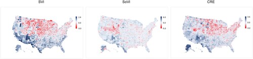
Figure 2 contains the choropleth maps of the social index data. The data are the sources’ latest releases: 2014 for SoVI, 2019 for CRE and 2020 for SVI. For the sake of comparison, all indices are converted to standard normal values. The SVI data reveal high social vulnerability among counties in the southern and coastal regions (blue colour). The SoVI data indicate a particularly high vulnerability along the US-Mexico border and in much of the state of Florida. The overall patterns of CRE data are similar to those of SVI, with the least vulnerable counties clustering in the midwestern region (red colour). All three indices point to high social vulnerability in the southwestern region close to the US-Mexico border and the state of Alaska. In addition to many counties in the Midwest, coastal communities in the northeastern region are relatively less vulnerable.

Figure 2. Maps of social index data.

Three maps showing the data of SVI, SoVI and CRE indices for US counties. Positive values in blue and negative values in red.

To further compare those social indices, Table 2 displays their pairwise Pearson correlation coefficients. The CRE index shows the highest correlations of 0.63 and 0.57 with SVI and SoVI, respectively. The correlation between SoVI and SVI is lower at 0.43. Overall, along with the observations in Figure 2, the simple correlation measures reveal the extent of disparities among the three composite indices due in part to their different constituent components as well as disparities in the extent of social vulnerability across US counties.

Table 2. Correlation matrix of social indices.

	SVI	SoVI	CRE
SVI	1.00	0.43	0.63
SoVI		1.00	0.57
CRE			1.00

Despite the burgeoning literature on the concept or theory of social vulnerability and the widespread application of its measures, it remains unclear how well those composite indices explain post-disaster outcomes. Among those exceptions, Bakkensen et al. (2017) highlight the relevance of different indices to different aspects of disasters, such as physical losses, fatalities and disaster declarations. Rufat et al. (2019) empirically evaluate SVI and SoVI based on an event study with various disaster outcome measures in the wake of Hurricane Sandy in 2015. They find substantial variation in the explanatory power of the two indices for a given disaster outcome as well as across different outcomes for a given index. One reason for the mixed evidence is a misalignment between the multidimensional nature of the indicators that make up the composite indices and the unidimensional disaster outcome measures.

2.3. Control variables

Other than pre-COVID community-level socioeconomic attributes, many factors could have brought about the observed discrepancies in recovery paths among US counties and their exposure to the economic disruptions caused by the COVID-19 pandemic. To minimise potential bias in our inferences on the social indices as our primary variable of interest, it is critical to control for those confounding factors. The first control variable we consider is the local COVID-19 caseload (number of cases per 1000 people), which might have stifled business activity with lower foot traffic, among other effects, at least during the early stage of the pandemic.

The second control variable is population density (the number of residents per square mile). Urban areas typically have a higher population density. During the early months of the pandemic, COVID-19 caseloads tended to be disproportionately high in city centres (Carozzi et al., 2022), leading to an ‘urban flight’ phenomenon in 2020 (Lee & Huang, 2022; Liu & Su, 2021). Moreover, Cutter et al. (2016) found distinctive geographic patterns of social vulnerability between urban and rural communities.

Another control variable is the ability to work from home, which has become popular, especially for some service industries since the nationwide lockdown during the early months of the pandemic. Remote work might have led to a wide range of consequences in different parts of the nation, from housing demand (Lee & Huang, 2022; Liu & Su, 2021; Mondragon & Wieland, 2022) to labour productivity (Bloom et al., 2022). An area or industry with a larger share of the remote workforce might be less exposed to disruptions caused by lockdowns and quarantines. On the other hand, workers who can work remotely do not necessarily need to live close to their workplace, giving rise to outmigration from cities with a high employment concentration (Althoff et al., 2022). The net effect of remote work on local economic recovery over time is therefore largely unknown.

We compiled data on the total share of employees working at home from the Bureau of Labor Statistics’ (BLS) American Time Use Survey (ATUS). Beginning in April 2022, the ATUS programme reported on a monthly basis the share of employed persons who ‘teleworked because of the coronavirus pandemic’ by industry. Before the pandemic, the ATUS data on workers who worked remotely for at least part of their workdays were collected annually beginning in 2003. For each county, estimates for the share of the total remote workforce were derived by multiplying the employment of individual sectors by their corresponding remote workforce shares in the ATUS reports for the nation. County-level employment data by sectors were obtained from the BLS Quarterly Census of Employment and Wages (QCEW) programme. The county-level remote workforce data drawn from the ATUS are highly correlated with occupational-based remote work compatibility data constructed under the methodology of Dingel and Neiman (2020). Their Pearson correlation coefficient is 0.88 for 2019 and about 0.95 for different months in 2020. The average remote workforce across US counties reached a peak of 29.3% in May 2020 and then gradually diminished to below 10% a year later.

There is strong evidence to support that a more diversified economy is more stable and economic diversification can attenuate an economic downturn in the wake of disasters (Coulson et al., 2020; Xiao & Drucker, 2013). We followed Coulson et al. (2020) to construct a measure of economic diversity for our county-level sample using QCEW sectoral employment data. In addition to economic diversity, we include in our empirical models the employment share of the ‘leisure and hospitality’ sector. This sector was hit hardest during the early months of the pandemic as a result of stay-at-home orders and travel restrictions.

The last confounding factor we consider arises from a wide range of government policy measures and interventions in response to COVID-19 outbreaks and the pandemic’s impact on the local economy. The diversity of government policies makes a comparison of outcome measures difficult. Nevertheless, the Oxford COVID-19 Government Response Tracker (OxCGRT) has tracked and compared common government responses consistently across countries and US states as well as over time (Hallas et al., 2021). For this study, we draw on OxCGRT’s two composite indices for individual states beginning in January 2020. The first is the policy stringency index, which reflects the strictness of closure and containment policies, such as lockdown restrictions and closures for schools, workplaces and public events. A higher value indicates stricter measures. Famiglietti and Leibovici (2021) find that states with stricter containment measures captured by the stringency index during the early months of the pandemic are associated with a short-term rise in unemployment but then faster labour market recoveries. The second index measures the extent of economic support to households, such as income support to people who lost their jobs and debt relief for people who were not able to make loan payments. The data are ordinal based on a scale of intensity. State governments’ responses to COVID-19 are likely to be exogenous to county-level conditions.

2.4. Empirical models

To investigate disparities in the COVID-induced economic downturn in early 2020 across US counties, we rely on a general regression framework as follows: (1) $\begin{array}{cc}{y}_i^{\ast }=\left|y_{\mathrm{it}-3}-y_{i0}\right|=b\cdot \mathrm{Inde}{x}_i+\mathit{D}\cdot \mathrm{Contro}{l}_i,& i\in \left[1,n\right]\end{array},$(1) where $\left|y_{\mathrm{it}-3}-y_{i0}\right|$ represents the overall change in the alternative economic outcome measures of county i between January 2020 as the baseline and April 2020 (t = 0) when the nationwide recession officially ended.¹ The size of the economic impact is measured alternatively by the percentage declines in employment and output levels and the increase in the unemployment rate. The term $\mathrm{Inde}{x}_i$ represents one of the three county-level indices measuring inherent social vulnerability. The expected sign is positive, meaning a county with a higher vulnerability score would be more susceptible to COVID-induced impacts. The term $\mathrm{Contro}{l}_i$ is a set of control variables described above, including a constant term (the share of the remote workforce, population density, the average daily COVID caseload in April 2020, an economic diversity measure, the share of hospitality employment and measures of the state government’s policy stringency and economic support in April 2020). The remote workforce, economic diversity and the share of the hospitality sector are based on the 2019 data. The terms b and D are free parameters for estimation. For data in levels (i.e., population density, COVID caseload and hospitality employment share), it is customary to deal with potential non-linearity in modelling relationships with log transformation.

The corresponding model for tracking the recovery phase of US counties through December 2022 follows the local projection specification (Jorda, 2005): (2) $\begin{array}{cc}{\tilde{y}}_{\mathrm{it}}=y_{\mathrm{it}}-y_{i0}=b_t\cdot \mathrm{Inde}{x}_i+{\mathit{D}}_t\cdot \mathrm{Contro}{l}_{\mathrm{it}-1},& t\in \left[1,32\right]\end{array},$(2) where variables with a subscript t represent time-varying data indexed by the month following the COVID-induced recession ending in April 2020. Given that the economies of more vulnerable counties are expected to lag other counties in the recovery phase, the expected sign for $\mathrm{Inde}{x}_i$ is negative in the regressions for employment and output and positive for unemployment. In addition to the dependent variables, some of the control variables vary over time: the share of the work-from-home workforce, the COVID caseload and the two state policy measures. To capture the dynamic impact on economic activity and to minimise potential endogeneity in the explanatory variables, the time-varying control variables enter the model with a one-month lag.

Yet the conventional least-squares estimation of Equations (1) and (2) abstracts from any indirect or spatial effects associated with interactions or spillovers between nearby counties. In reality, local labour markets and economies tend to be interrelated, especially in the wake of a disaster. For instance, Belasen and Polachek (2009) describe how communities in the state of Florida hit directly by a hurricane affected the labour supply and wages in their surrounding areas. As people commute to work, counties next to each other tend to share the same impacts of COVID-19 outbreaks. On the other hand, local regulations and public services, such as school closures and online class delivery, vary from one community to another.

To account for spatial autocorrelation and spatial heterogeneity in model relationships, we first consider the GWAR framework (Geniaux & Martinetti, 2018), which extends the least-squares or ‘global’ models in two directions simultaneously: (1) incorporating spatial autocorrelation in the dependent variable and (2) estimating parameters ‘locally’ for different geographic locations. Following the conventional notation, an extension of Equations (1) and (2) to GWAR can be expressed, respectively, as: (3) $y_i^{\ast }=\rho \left(u_i,v_i\right)\sum _{j=1}^n{w}_{\mathrm{ij}}^1{y}_j^{\ast }+b\left(u_i,v_i\right)\cdot \mathrm{Inde}{x}_i+\mathit{D}\left(u_i,v_i\right)\cdot \mathrm{Contro}{l}_i,$(3) (4) ${\tilde{y}}_{\mathrm{it}}=\rho \left(u_i,v_i\right)\sum _{j=1}^n{w}_{\mathrm{ij}}^1{\tilde{y}}_{\mathrm{jt}}+b\left(u_i,v_i\right)\cdot \mathrm{Inde}{x}_i+\mathit{D}\left(u_i,v_i\right)\cdot \mathrm{Contro}{l}_{\mathrm{it}-1},$(4) where $\left(u_i,v_i\right)$ denotes the respective longitude and latitude coordinates (county centroid) of county i, and the parameters $\rho \left(u_i,v_i\right),b\left(u_i,v_i\right),$ and $\mathit{D}\left(u_i,v_i\right)$ reflect values for that county. In contrast to fixed parameter estimates for all locations in ‘global’ models such as Equations (1) and (2), the above GWAR equations capture heterogeneous local effects by allowing the parameters to vary across data observations of different counties.

In Equations (3) and (4), $\rho \left(u_i,v_i\right)$, is a scalar parameter called the spatial autoregressive (SAR) parameter, and $w_{\mathrm{ij}}^1$ is an element of a spatial weight matrix ${\mathit{W}}^1$ that determines the spatial structure between two locations. In line with the first law of geography, this spatial weight matrix assumes that data points closer to county i have a greater effect in estimating a parameter than observations located farther from that county (Fotheringham et al., 2002). Our specific weighting scheme draws on the ‘adaptive’ bandwidth scheme so that the distance for capturing the same number of neighbouring counties varies across different counties. This specification reflects different geographical sizes of counties in the United States. For county i, the weight of data observations of another county j is given by an adaptive Gaussian distance decay-based weighting function: (5) $w_{\mathrm{ij}}^1=\exp \left(-{\displaystyle \frac{d_{\mathrm{ij}}^2}{h_i^2}}\right)$(5) where $d_{\mathrm{ij}}^2=\left[\right(u_i-u_j{)}^2+\left(v_i-v_j{)}^2\right]$ is the Euclidean distance between county i and county j, and $h_i$ is the spatial bandwidth (or window size) for county i. The optimal spatial bandwidth is identified based on a goodness-of-fit criterion – the Akaike information criterion (AIC) corrected for small sample sizes (Fotheringham et al., 2002).

Essentially, the spatially lagged dependent variable (${\mathit{W}}^1{y}^{\ast }$ and ${\mathit{W}}^1{\tilde{y}}_{\mathit{t}}$) is the key element of the SAR model, which incorporates information from nearby counties (LeSage & Pace, 2009). However, SAR remains a ‘global’ model that does not account for unobserved spatial heterogeneity. Model relationships may be unevenly distributed across counties or broad regions in the United States. As a common approach to characterising unobservable or hidden spatial heterogeneity in data relationships, geographically weighted regression (GWR) estimates model parameters ‘locally’ for individual locations. The GWAR framework allows us to explore economic spillovers or clustering effects across counties within a region in the United States while allowing for disparities across regions. Wu et al. (2014), and Lee and Huang (2022) find this model helpful for characterising varying spatial patterns in local housing markets across different US regions.

Still, economic relationships likely evolve over time as well as over space. This is especially true for the case of the COVID-19 pandemic, which precipitated a historically deep economic contraction in early 2020 with uneven recovery across the nation in the following two years. To explore the temporal effects during the pandemic, we adopt the framework developed by Fotheringham et al. (2015) and Huang et al. (2010). The GTWAR model, which accounts for spatial dependence and ‘local’ effects in both space and time, can be expressed as: (6) $y_i^{\ast }=\rho \left(u_i,v_i,t_i\right)\sum _{j=1}^n{w}_{\mathrm{ij}}^1{y}_j^{\ast }+b\left(u_i,v_i,t_i\right)\cdot \mathrm{Inde}{x}_i+\mathit{D}\left(u_i,v_i,t_i\right)\cdot \mathrm{Contro}{l}_i,$(6) (7) ${\tilde{y}}_{\mathrm{it}}=\rho \left(u_i,v_i,t_i\right)\sum _{j=1}^n{w}_{\mathrm{ij}}^1{\tilde{y}}_{\mathrm{jt}}+b\left(u_i,v_i,t_i\right)\cdot \mathrm{Inde}{x}_i+\mathit{D}\left(u_i,v_i,t_i\right)\cdot \mathrm{Contro}{l}_{\mathrm{it}-1},$(7) here the parameters $\rho \left(u_i,v_i,t_i\right),a\left(u_i,v_i,t_i\right),b\left(u_i,v_i,t_i\right),$ and $\mathit{D}\left(u_i,v_i,t_i\right)$ are specific to the space–time location of county i with t corresponding to period t of county i’s data observations.

To estimate the GTWAR model, we follow the two-stage least-squares estimation procedure suggested by Wu et al. (2014). The spatial weights become the space–time distance function of $\left(u_i,v_i,t_i\right)$. Because of the different scale effects of location and time an ellipsoidal coordinate system is used to measure the spatial distance between a regression point and its surrounding data points. The spatial–temporal distance $d_{\mathrm{ij}}^{\mathrm{ST}}$ can be defined as a linear combination of the spatial distance $d_{\mathrm{ij}}^S$ and temporal distance $d_{\mathrm{ij}}^T$: (8) $\begin{array}{rl}(d_{\mathrm{ij}}^{\mathrm{ST}}{)}^2& =\lambda (d_{\mathrm{ij}}^S{)}^2+\mu (d_{\mathrm{ij}}^T{)}^2\\ & =\lambda \left[\right(u_i-u_j{)}^2+\left(v_i-v_j{)}^2\right]+\mu (t_i-t_j{)}^2\end{array}$(8) where the parameters $\lambda$ and $\mu$ are scale factors to balance the different scale effects used to measure spatial and temporal distance, respectively. The diagonal elements of the spatial–temporal weight matrix are: (9) $\begin{array}{rl}{w}_{\mathrm{ij}}^2& =\exp \left\{-\left({\displaystyle \frac{{\left(d_{\mathrm{ij}}^{\mathrm{ST}}\right)}^2}{h_{\mathrm{ST}}^2}}\right)\right\}\\ & =\exp \left\{-\left({\displaystyle \frac{{\left(d_{\mathrm{ij}}^S\right)}^2}{h_S^2}}\right)\right\}\times \exp \left\{-\left({\displaystyle \frac{{\left(d_{\mathrm{ij}}^T\right)}^2}{h_T^2}}\right)\right\}\\ =w_{\mathrm{ij}}^S\times w_{\mathrm{ij}}^T\end{array}$(9) where $h_S$, $h_T$,$h_{\mathrm{ST}}$ are spatial, temporal and spatial–temporal bandwidths, respectively. If the parameter $\mu$ is zero, then GTWAR reduces to GWAR without the consideration of temporal variation.

3. EMPIRICAL RESULTS

3.1. Economic downturn

Our empirical work begins with estimating cross-section models for the economic impact of COVID-19 across US counties during the 2020 nationwide recession. Table 3 presents the least-squares estimation results of a model specification with alternative social vulnerability indices and the control variables described in the previous section. The alternative measures of the dependent variable, represented by $y_i^{\ast }$ in Equation (1), are the absolute differences between the values in April 2020 and the values in January 2020. Given the state-level instead of county-level data for the government policy variables that potentially result in heteroskedasticity in model regressions, the t-statistics are derived from standard errors that are robust to clustering errors across states.

Table 3. Least-squares regression results for economic impact models.

	SVI			SoVI			CRE
	Coeff.	t-stat	%R^2	Coeff.	t-stat	%R^2	Coeff.	t-stat	%R^2
A. Employment
Social index	0.10	(1.19)	0.02	−0.03	(0.21)	0.01	0.45	(4.69)*	0.07
Remote work	−0.51	(2.86)*	0.07	−0.51	(2.88)*	0.07	−0.51	(2.85)*	0.07
Density	3.11	(6.65)*	0.32	3.12	(6.30)*	0.33	3.20	(7.09)*	0.32
COVID	0.08	(1.48)	0.02	0.08	(1.45)	0.02	0.08	(1.50)	0.02
Diversity	2.14	(3.42)*	0.06	2.12	(3.36)*	0.06	1.74	(2.74)*	0.05
% Hospitality	1.37	(7.80)*	0.23	1.36	(7.75)*	0.23	1.33	(7.67)*	0.22
Policy stringency	1.50	(16.83)*	0.26	1.51	(17.18)*	0.27	1.44	(16.07)*	0.24
Economic support	−0.02	(0.23)	0.01	−0.05	(0.54)	0.01	0.05	(0.53)	0.01
Adjusted R^2	0.33			0.33			0.33
Moran’s I	50.54*			50.79*			50.04*
B. Unemployment
Social index	0.05	(1.74)***	0.01	0.22	(3.05)*	0.05	0.19	(2.60)*	0.04
Remote work	−0.06	(0.77)	0.02	−0.08	(0.97)	0.01	−0.06	(0.77)	0.01
Density	2.68	(8.89)*	0.37	2.73	(8.61)*	0.36	2.72	(8.89)*	0.37
COVID	0.08	(2.00)**	0.03	0.07	(1.80)***	0.03	0.08	(2.01)**	0.03
Diversity	2.80	(6.15)*	0.11	2.72	(5.98)*	0.11	2.62	(5.77)*	0.10
% Hospitality	0.90	(8.34)*	0.21	0.90	(8.36)*	0.20	0.89	(8.22)*	0.20
Policy stringency	0.66	(10.04)*	0.16	0.67	(10.32)*	0.16	0.64	(9.61)*	0.15
Economic support	0.36	(5.17)*	0.09	0.36	(5.41)*	0.09	0.39	(5.52)*	0.09
Adjusted R^2	0.34			0.34			0.34
Moran’s I	53.16*			53.07*			53.23*
C. Output
Social index	0.10	(0.01)	0.02	0.12	(0.73)	0.02	0.34	(2.97)*	0.05
Remote work	−0.64	(3.06)*	0.09	−0.65	(3.10)*	0.09	−0.64	(3.04)*	0.09
Density	3.48	(6.26)*	0.35	3.50	(5.68)*	0.35	3.53	(6.51)*	0.34
COVID	0.23	(3.45)*	0.07	0.22	(3.35)*	0.06	0.23	(3.49)*	0.06
Diversity	4.45	(6.45)*	0.13	4.41	(6.41)*	0.12	4.17	(6.02)*	0.11
% Hospitality	0.53	(3.02)*	0.09	0.53	(3.03)*	0.09	0.50	(2.92)*	0.08
Policy stringency	1.51	(14.07)*	0.24	1.51	(14.16)*	0.25	1.46	(13.61)*	0.24
Economic support	0.08	(0.82)	0.01	0.09	(0.93)	0.02	0.15	(1.53)	0.03
Adjusted R^2	0.22				0.22				0.23
Moran’s I	42.69*			42.52*			42.53*

Notes: Absolute values of t-statistics with robust standard errors are listed in parentheses.*,**, and*** denote statistical significance at the 1%, 5%, and 10% levels, respectively.

According to the estimation results, the impact on employment is associated only with the CRE index. For unemployment, the parameter estimates of all three social indices are statistically meaningful. The positive estimates indicate that counties with higher social vulnerability tended to experience higher unemployment in the wake of the COVID-induced recession. In the regressions for output, similar to the results for employment, only the estimate for CRE out of the three social indices is statistically meaningful.

For the control variables, most coefficient estimates are statistically significant with the expected signs. For instance, the pandemic disproportionately hit more densely populated counties than others, highlighting COVID-19’s impact on urban versus rural areas. Also, counties with a lower share of remote workforce, more exposure to the hospitality sector and more restrictive government lockdown policies tended to experience a more severe economic downturn. Yet there are some exceptions. First, the estimates for the COVID caseload are not statistically significant in explaining employment impacts. Second, the share of the remote workforce has no meaningful explanatory power in the unemployment regressions. Third, the estimates for the variable representing state governments’ economic support are not statistically meaningful in the employment and output regressions.

Gauged by the adjusted R²’s as measures of the overall goodness of fit, the set of regressors collectively explains between 23% and 34% of cross-county changes in economic outcomes. Given the multitude of regressors in the model, it is interesting to find out which determinants are more helpful than others in explaining the exposure of local economic activity to the pandemic. We accomplish this by applying the Shapley–Owen decomposition to measure each regressor’s contribution to the overall R²’s (Israeli, 2007). As shown in the third column of each panel in Table 2, population density explains most of the cross-sectional variation in all three economic outcomes, followed by policy stringency and the presence of the hospitality sector. By comparison, the three social vulnerability indices contribute the least to variation in local economic outcomes during the 2020 recession.

However, the z-scores of Moran’s I test for spatial dependence strongly reject the null hypothesis of no spatial correlation in the residuals of regressions. In other words, regression errors are correlated with the spatial linkages of the observations of the dependent variables, leading to biased and inconsistent parameter estimates (Basile & Minguez, 2018). In Section 3.3 below, we will deal with this drawback with a spatial lag model specification.

3.2. Economic recovery

Next, we look at local economic outcomes following the end of the 2020 recession. Least-squares regressions of the local projection model depicted by Equation (2) are run for each month between May 2020 and December 2022. All explanatory variables in the recovery model are the same as those in the impact model, except that the time-varying control variables enter the model with a one-month lag. Figure 3 plots the estimated parameters of the three alternative social vulnerability indices. The shaded areas around the point estimates delineate the 95% confidence bands. For the employment regressions, the parameter estimates of all three social indices are mostly negative and statistically significant. The estimates for the SVI and SoVI tend to drift downward throughout the observation period, suggesting that counties with higher social vulnerability experienced a slower employment recovery over time in the wake of the 2020 recession.

Figure 3. Least-square estimates for social indices in recovery models.

Nine line graphs showing the least-squares parameter estimates of SVI, SoVI and CRE indices for employment, unemployment and output in each month between May 2020 and December 2022. Each line of point estimates is surrounded by a shaded zone representing the 95% confidence interval.

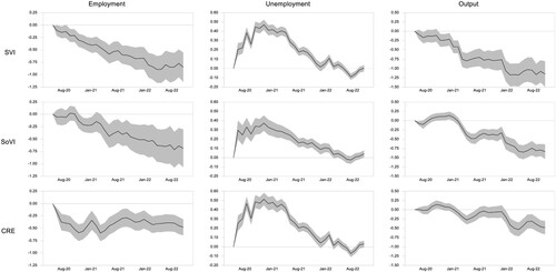
The dynamic patterns of the estimates among the three social indices are also similar for the unemployment regressions. The parameter estimates rise over the first six months of the recovery phase and after that inch down towards zero towards the end of the observation period. Positive estimates indicate that unemployment was relatively higher among counties with higher social vulnerability. The plots support the contribution of social vulnerability in explaining disparities in local unemployment only through the end of 2021.

The plots for the output regressions are similar to those for employment. Overall, the parameter estimates for social indices are negative and continue to decline as time passes. One notable observation is the estimate for CRE, which aligns with the estimates for SVI and SoVI in support of an increasing role of social vulnerability in explaining local economic recovery over time.

To provide a snapshot of the estimated models for economic recovery, Table 4 shows the least-squares estimation results for the final month of the observation period (i.e., December 2022). The adjusted R²’s are as high as 0.75 (unemployment), though economic support from state governments contributes the most to the model’s overall explanatory power. The social indices’ shares of the overall R²’s are notably higher than their counterparts in the impact models and their parameters are all statistically meaningful. Contrary to their results for explaining COVID-19’s economic impacts (Table 3), population density no longer explains variation in local employment and output, reflecting the negligible difference between urban and rural areas in their exposure to COVID-19 outbreaks. By the end of 2022, economic diversification did not help explain local economic performance when the hospitality sector emerged as a key economic driver. The estimates for the ‘impact’ variable ($y_i^{\ast }$) suggest that communities hit harder during the downturn also tended to bounce back more strongly. The state policy variables also help explain local recovery, particularly in output.

Table 4. Least-squares regression results for economic recovery models, December 2022.

	SVI			SoVI			CRE
	Coeff.	t-stat	%R^2	Coeff.	t-stat	%R^2	Coeff.	t-stat	%R^2
A. Employment
Social index	−0.85	(5.74)*	0.15	−0.69	(3.58)*	0.10	0.46	(4.20)*	0.07
Remote work	38.48	(1.78)***	0.04	22.80	(1.04)	0.03	39.58	(1.80)***	0.04
Density	0.17	(0.35)	0.02	−0.64	(1.79)***	0.06	−0.45	(1.28)	0.04
COVID	−0.13	(0.78)	0.02	−0.09	(0.61)	0.02	−0.15	(0.96)	0.02
Diversity	−1.44	(2.15)**	0.04	−2.57	(4.93)*	0.07	−2.99	(5.69)*	0.08
% Hospitality	0.06	(1.26)	0.01	0.37	(1.67)***	0.06	0.36	(1.65)***	0.06
Policy stringency	−1.82	(4.72)*	0.04	0.07	(0.78)	0.01	0.04	(0.41)	0.01
Economic support	0.83	(1.60)	0.01	0.14	(0.85)	0.03	0.23	(1.45)	0.04
Impact ($y_i^{\ast }$)	1.01	(14.11)*	0.66	0.93	(22.05)*	0.66	0.93	(21.11)*	0.64
Adjusted R^2	0.56			0.49			0.49
Moran’s I	19.74*			19.03*			19.08*
B. Unemployment
Social index	0.03	(1.72)	0.01	0.04	(2.17)**	0.03	0.03	(1.79)***	0.02
Remote work	−7.87	(2.27)**	0.03	−8.32	(2.43)*	0.03	−8.30	(2.41)*	0.03
Density	−0.06	(1.95)***	0.03	−0.06	(1.70)***	0.02	−0.06	(1.76)***	0.02
COVID	0.11	(5.10)*	0.06	0.11	(5.12)*	0.06	0.11	(5.14)*	0.06
Diversity	0.01	(0.14)	0.00	0.01	(0.08)	0.00	−0.01	(0.07)	0.00
% Hospitality	0.01	(0.07)	0.00	0.01	(0.01)	0.00	0.01	(0.15)	0.00
Policy stringency	0.15	(7.62)*	0.11	0.15	(7.52)*	0.11	0.15	(7.75)*	0.11
Economic support	−0.06	(3.73)*	0.05	−0.06	(3.59)*	0.05	−0.06	(3.56)*	0.05
Impact ($y_i^{\ast }$)	−0.91	(14.34)*	0.71	−0.91	(14.71)*	0.69	−0.91	(14.16)*	0.70
Adjusted R^2	0.74			0.75			0.75
Moran’s I	61.60*			61.55*			61.57*
C. Output
Social index	−1.15	(6.70)*	0.20	−0.84	(4.17)*	0.18	−0.54	(2.70)*	0.09
Remote work	25.22	(1.11)	0.03	32.12	(1.42)	0.04	35.41	(1.55)	0.05
Density	0.29	(0.63)	0.03	0.02	(0.01)	0.00	0.09	(0.17)	0.01
COVID	0.02	(0.03)	0.01	−0.03	(0.24)	0.01	−0.07	(0.45)	0.01
Diversity	−2.15	(2.87)*	0.06	−1.56	(2.20)*	0.05	−1.20	(1.81)***	0.04
% Hospitality	0.36	(1.69)***	0.08	0.47	(2.33)**	0.10	0.47	(2.36)**	0.11
Policy stringency	−2.02	(4.70)*	0.04	−2.07	(4.85)*	0.04	−2.06	(4.75)*	0.05
Economic support	1.19	(1.72)***	0.02	0.89	(1.27)	0.01	1.18	(1.78)***	0.02
Impact ($y_i^{\ast }$)	0.64	(11.59)*	0.55	0.65	(11.82)*	0.57	0.66	(11.76)*	0.62
Adjusted R^2	0.47			0.46			0.46
Moran’s I	18.86*			18.79*			18.28*

Notes: Absolute values of t-statistics with robust standard errors are listed in parentheses.*,**, and*** denote statistical significance at the 1%, 5%, and 10% levels, respectively.

Overall, the regression results for economic outcomes during the recovery period improve over their corresponding results during the downturn. The estimates for the social indices support the role of pre-COVID social vulnerability characteristics in explaining variation in economic performance across counties during the second year of the recovery phase. The results are robust to the presence of a wide variety of control variables, including state government policy responses.

It is, however, noteworthy that the explanatory power of different explanatory variables differs remarkably between the regressions for April 2020 and December 2022. Moran’s I test statistics indicate the presence of spatial autocorrelation in all regression models. Despite the strong evidence in support of the role of social vulnerability in local economic recovery on average, the ‘global’ regression results may well mask disparities across counties. This drawback is critical for understanding the impacts of social vulnerability, which has been found to vary across US regions (Cutter et al., 2014, 2016; Park & Xu, 2020). In light of these findings, we will apply the GTWAR model to account for hidden spatial and temporal effects.

3.3. GTWAR results

To discover cross-sectional heterogeneity and autocorrelation behind the average effects of social vulnerability on local economic outcomes over the course of the pandemic, we apply GTWAR captured by Equations (6) and (7). Table 5 reports the GTWAR results analogous to the least-squares model for estimating the local economic downturn (Table 3). Each panel displays the summary statistics of the local parameter estimates for one of the three alternative social indices and the spatially lagged dependent variable (${\mathit{W}}^1{y}^{\ast }$). The ‘local’ regression estimates are conditional on the identified spatial and temporal bandwidths that best fit the data.

Table 5. GTWAR results for impact models, April 2020.

	SVI						SoVI						CRE
		Std.	Min.	Median	Max.			Std.	Min.	Median	Max.			Std.	Min.	Median	Max.
A. Employment
Social index		0.18	−0.82	−0.08	0.65			0.15	−0.49	−0.03	0.56			0.20	−0.81	−0.03	0.95
Spatial lag		0.15	0.10	0.66	0.95			0.16	0.03	0.66	0.94			0.15	0.03	0.67	0.94
Adjusted R^2	0.93						0.93						0.93
Spatial h	224						204						224
Temporal h	1						1						1
B. Unemployment
Social index		0.17	−0.67	0.06	0.76			0.17	−0.42	0.08	0.71			0.21	−0.44	0.05	1.51
Spatial lag		0.16	0.19	0.70	0.99			0.17	0.19	0.69	0.98			0.16	0.16	0.69	0.98
Adjusted R^2	0.92						0.93						0.93
Spatial h	234						234						224
Temporal h	1						1						1
C. Output
Social index		0.19	−0.86	−0.05	0.59			0.15	−0.59	−0.01	0.50			0.18	−0.53	−0.01	0.84
Spatial lag		0.16	0.10	0.62	0.84			0.16	0.12	0.62	0.89			0.14	0.19	0.64	0.86
Adjusted R^2	0.84						0.84						0.86
Spatial h	226						224						266
Temporal h	1						1						1

Notes: The models are estimated for the respective measures of economic activity with one of the three alternative social indices and a set of control variables (the remote workforce, population density, COVID caseload, economic diversity, the hospitality employment share, policy stringency, economic support and the corresponding economic impact).

All adjusted R²’s are considerably higher than their counterparts from least-squares or ‘global’ regressions in Table 3. Improvement in the predictive accuracy of SAR and GWR models is well documented in the spatial modelling literature (e.g., Fotheringham et al., 2015), reflecting the prevalence of autocorrelation and heterogeneity in geographical data observations. The bandwidth that best fits the spatial data ranges between 204 and 266 counties, reflecting variation in model relationships across broad regions (given an average of 62 counties among the 50 states). The temporal bandwidth of one in all models supports the benefit of incorporating one-month-lagged information in estimating economic outcomes in April 2020, given the abrupt and short-lived nature of the COVID-induced recession.

For all three economic outcome measures, the estimates of the spatial lag parameters are positive for all counties. This means that the overall economy of an individual county was directly associated with that of its surrounding counties during the recession. Yet it is also important to observe that some local SAR estimates are as low as 0.03, meaning very low spatial dependence for some counties.

The summary statistics of the social indices’ ‘local’ parameter estimates also reveal the varying role of inherent social vulnerability across counties in explaining their exposure to COVID-induced economic shocks. Contrary to the mixed results in the least-squares regressions, the median local parameter estimates are negative in the employment and output equations and positive in the unemployment equation. This means that a typical county with higher social vulnerability experienced a smaller impact of COVID-19 on employment and output during the nationwide recession, but it also witnessed higher unemployment. However, the widespread cross-sectional distribution of local parameter estimates in most panels, as evidenced by the standard deviation and the range between the minimum and maximum values, suggests that it is instructive to take a close look at the spatial patterns of the estimates across the US.

Figure 4 contains the Choropleth maps of GTWAR estimates for the social indices. For each county, the ‘local’ estimates also include the ‘indirect’ spatial effects of its neighbours, as captured by its spatial lag parameter estimate (LeSage & Pace, 2009). Only counties with parameters that are statistically significant at the 10% level or better are visible. Beneath each map are the numbers of counties with positive and negative estimates. Regional disparities in local parameter estimates are apparent. Among the three social indices, the local estimates are most consistent for their relationships with unemployment. The estimated relationship is positive for most counties in the eastern United Sates and negative in the state of Alaska and some regions in the Pacific Northwest. The number of counties with a positive estimate (blue colour) far outweighs the number of counties with a negative estimate (red colour).

Figure 4. GTWAR estimates for social indices in impact models, April 2020.

Notes: The maps show local parameter estimates for counties that are significant at the 10% level or better. The figure following a ‘+’ sign is the number of counties with a positive local parameter estimate and the figure following a ‘–’ sign is the number of counties with a negative local parameter estimate.

Nine maps of US counties showing GTWAR estimates for SVI, SoVI and CRE indices in the impact models for employment, unemployment and output. Positive estimates in blue and negative estimates in red. Below each map are the total numbers of counties with positive and negative estimates.

In line with the ‘global’ regression results in Table 3, the local estimates for employment and output are equivocal. A positive association between social vulnerability and COVID-19’s impact on employment and output is found in the northeastern and Great Lakes regions. Negative estimates spread across some southwestern regions, including the state of California and counties along the US-Mexico border. Those counties tend to have relatively high social vulnerability scores (see Figure 2). This means that highly vulnerable counties in those regions did not experience disproportionate impacts on their labour markets and output.

Next, we apply GTWAR to the subsequent recovery phase. Table 6 shows the estimation results of our primary interest for the final month of the observation period, namely December 2022. Like the GTWAR results for estimating economic impacts (Table 5), the adjusted R²’s improve over their corresponding statistics of the ‘global’ models (Table 4). All selected temporal bandwidths that best fit the data are two months. The optimal spatial bandwidths between 112 and 199 indicate spatial patterns over broad US regions, but they are smaller than the regions identified for estimating the economic downturn (see Table 5).

Table 6. GTWAR results for recovery models, December 2022.

	SVI						SoVI						CRE
		Std.	Min.	Median	Max.			Std.	Min.	Median	Max.			Std.	Min.	Median	Max.
A. Employment
Social index		0.13	−0.60	−0.06	0.62			0.13	−0.89	−0.05	0.33			0.14	−0.51	−0.03	0.84
Spatial lag		0.20	−0.55	0.22	0.70			0.20	−0.50	0.23	0.70			0.20	−0.50	0.23	0.71
Adjusted R^2	0.98						0.98						0.98
Spatial h	149						149						149
Temporal h	2						2						2
B. Unemployment
Social index		0.04	−0.21	0.00	0.17			0.04	−0.15	−0.01	0.14			0.05	−0.24	−0.01	0.15
Spatial lag		0.10	−0.26	0.05	0.52			0.10	−0.33	0.05	0.54			0.10	−0.25	0.05	0.51
Adjusted R^2	0.99						0.99						0.99
Spatial h	112						112						112
Temporal h	2						2						2
C. Output
Social index		0.13	−0.81	−0.08	0.20			0.15	−1.09	−0.07	0.20			0.13	−0.60	−0.04	0.50
Spatial lag		0.19	−0.39	−0.28	0.70			0.20	−0.40	−0.28	0.71			0.20	−0.40	−0.28	0.72
Adjusted R^2	0.97						0.97						0.97
Spatial h	199						199						199
Temporal h	2						2						2

Notes: The models are estimated for the respective measures of economic activity with one of the three alternative social indices and a set of control variables (the remote workforce, population density, COVID caseload, economic diversity, the hospitality employment share, policy stringency, economic support and the corresponding economic impact).

The estimation results for the spatial lag contrast the corresponding results in Table 5. Instead of all positive estimates, the SAR estimates are negative for some counties, reflecting divergent economic trends between those counties and their neighbours. In most cases, the median local parameter estimates are near zero and the maximums and minimums not only spread out widely but are also in opposite signs.

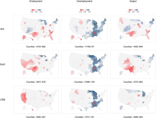
Figure 5 displays how the relationships between social vulnerability and local economic outcomes varied across the United States in December 2022. In contrast to the observations during the COVID-19 recession (see Figure 4), the spatial distributions over the United States are similar among the three social indices. The patterns for estimating the impact on employment and output are also considerably similar. Reflecting the prominence of social vulnerability in explaining local economic recovery, the counties with negative estimates far exceed the counties with positive estimates. In addition to Alaska, negative estimates cluster among some states in the Rocky Mountain region, including Idaho, Nevada and Utah, and the southwestern region, such as Arizona and Mexico. In those US regions, counties with higher social vulnerability scores experienced lower employment and output than counties with lower social vulnerability scores.

Figure 5. GTWAR estimates for social indices in recovery models, December 2022.

Notes: The maps show local parameter estimates for counties that are significant at the 10% level or better. The figure following a ‘+’ sign is the number of counties with a positive local parameter estimate and the figure following a ‘–’ sign is the number of counties with a negative local parameter estimate.

Nine maps of US counties showing GTWAR estimates for SVI, SoVI and CRE indices in the recovery models for employment, unemployment and output. Positive estimates in blue and negative estimates in red. Below each map are the total numbers of counties with positive and negative estimates.

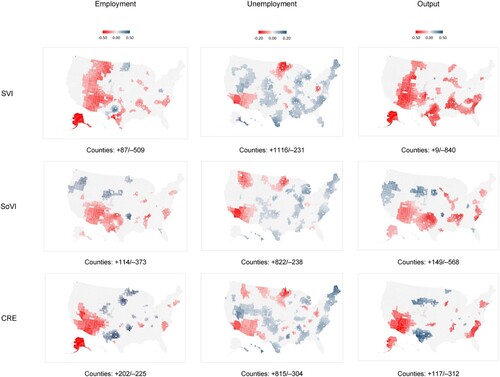
In the maps for unemployment, the local parameter estimates are also predominately positive, meaning higher unemployment rates among counties with inherently higher social vulnerability. Yet their spatial patterns are distinctive from those in the maps for employment and output. Positive estimates spread along the coastal regions of the Atlantic and Gulf of Mexico. Negative estimates cluster in the southwestern region, such as southern California and the states of Nevada and Arizona.

Overall, the GTWAR estimation results confirm the role that social vulnerability played in local economic recovery on average. Yet the inference from conventional global model regressions is apparently not informative about counties that experienced disparate economic outcomes during the pandemic. The three alternative social vulnerability measures are most relevant to local economic performance in parts of the southwestern and northeastern regions in both the recession and recovery periods. For many counties in other regions, such as the Pacific Northwest and Midwest, the pre-COVID social vulnerability conditions captured by the three composite indices fail to explain their economic experiences.

4. CONCLUSION

Social vulnerability is at the crux of recent discussions about how local communities navigate disasters like the COVID-19 pandemic. We have first followed the conventional ‘global’ regression approach to empirically evaluating three community-based social vulnerability indices in the context of local economic performance during the pandemic. This approach generates equivocal results regarding the role of social vulnerability in the local economic downturn triggered by the onset of COVID-19 outbreaks. Discrepancies in the regression results for the roles of the three alternative indices on different counties’ exposure to COVID-19’s immediate impact complement recent studies that question the empirical validity of those social vulnerability constructs (e.g., Rufat et al., 2019).

On the other hand, empirical results infer that counties with higher social vulnerability tended to bounce back less swiftly in the wake of the pandemic-induced recession. Our work further contributes to the related literature by exploring the varying role of social vulnerability within and across US regions as well as over the course of the pandemic. Inferences based on ‘global’ regression models are informative only about social vulnerability among US counties on average. Estimation results from those conventional models mask the presence of unobserved heterogeneity and spillovers of economic shocks across counties or regions. We have resolved such drawbacks by following the geographically weighted approach to estimating ‘local’ parameters for individual counties simultaneously with the consideration of spatial dependence and temporal effects.

The GTWAR model generates local parameter estimates to reveal the extent of spatial heterogeneity in the relationship between inherent sociodemographic attributes and local economic outcomes throughout the pandemic while allowing for spatial dependence. Exposure to COVID-19’s initial economic shocks was positively related to social vulnerability as expected among counties in the Great Lakes and New England regions in the northeastern United States. Social vulnerability also helps explain the pace of local economic recovery in parts of the west, especially the southwestern region.

In light of the sizeable number of counties with local parameter estimates opposite to the expected sign, the GTWAR model generated overall mixed results in support of the validity of the community-level measures of sociodemographic attributes as a one-size-fits-all measure of local economic vulnerability. For a considerable number of counties, those composite indices alone fail to characterise local economic performance during the COVID-19 pandemic. This implies that even if those indices are reliable screening tools for policymakers and government officials to assess the inherent vulnerability of a broad region to disasters, they should be applied to individual communities circumspectly. This is particularly crucial for those composite measures aimed at capturing the inherently multidimensional nature of social vulnerability, which is a plausible factor behind the mixed evidence on their empirical relevance in the pandemic.

The mixed empirical findings in this study also highlight the importance of continuing to evaluate the relevance of social vulnerability indices to different types of disasters in the future. Given the observed disparities as well as similarities among the composite social indices, more fruitful research could be in the direction of identifying individual community attributes or indicators that contribute most to vulnerability to a targeted disaster.

The temporal dimension of GTWAR has allowed us to unravel the temporal dynamic of local economic recovery in addition to spatial effects across counties. Unlike the recession in 2020, the spatial distribution of local parameter estimates over the recovery period is quite consistent among the three social indices. Nevertheless, the nuanced differences in their spatial patterns throughout the pandemic highlight the distinctive roles of different sociodemographic attributes behind the composite indices for individual counties at different stages of the economic cycle.

DISCLOSURE STATEMENT

No potential conflict of interest was reported by the author(s).

Notes

1 We selected January 2020 for measuring the baselines but the empirical results do not alter meaningfully with other selections, such as February 2020 and the monthly averages of 2019. Similarly, rather than April 2020 for all counties, we have found no noticeably different results if we select the month in 2020 with the largest impact measure for individual counties.

REFERENCES

- Althoff, L., Eckert, F., Ganapati, S., & Walsh, C. (2022). The geography of remote work. Regional Science and Urban Economics, 93, 103770. https://doi.org/10.1016/j.regsciurbeco.2022.103770
- Bakkensen, L. A., Fox-Lent, C., Read, L. K., & Linkov, I. (2017). Validating resilience and vulnerability indices in the context of natural disasters. Risk Analysis, 37(5), 2017. https://doi.org/10.1111/risa.12677
- Basile, R., & Minguez, R. (2018). Advances in spatial econometrics: Parametric vs. semiparametric spatial autoregressive models. In P. Commendatore, I. Kubin, S. Bougheas, A. Kirman, M. Kopel, & G. Bischi (Eds.), The economy as a complex spatial system, springer proceedings in complexity (pp. 81–106). Cham: Springer. https://doi.org/10.1007/978-3-319-65627-4_4.
- Belasen, A. R., & Polachek, S. W. (2009). How disasters affect local labor markets: The effects of hurricanes in Florida. Journal of Human Resources, 44(1), 251–276. https://doi.org/10.1353/jhr.2009.0014
- Bergstrand, K., Mayer, B., Brumback, B., & Zhang, Y. (2015). Assessing the relationship between social vulnerability and community resilience to hazards. Social Indicators Research, 122(2), 391–409. https://doi.org/10.1007/s11205-014-0698-3
- Bloom, N., Bunn, P., Mizen, P., Smietanka, P., & Thwaites, G. (2022). The impact of COVID-19 on productivity. National Bureau of Economic Research, Working Paper, 28233.
- Carozzi, F., Provenzano, S., & Roth, S. (2022). Urban density and COVID-19: Understanding the US experience. The Annals of Regional Science, https://doi.org/10.1007/s00168-022-01193-z
- Coulson, N. E., McCoy, S. J., & McDonough, I. K. (2020). Economic diversification and the resiliency hypothesis: Evidence from the impact of natural disasters on regional housing values. Regional Science and Urban Economics, 85, 103581. https://doi.org/10.1016/j.regsciurbeco.2020.103581
- Cutter, S. L., Ash, K. D., & Emrich, C. T. (2014). The geographies of community disaster resilience. Global Environmental Change, 29, 65–77. https://doi.org/10.1016/j.gloenvcha.2014.08.005
- Cutter, S. L., Ash, K. D., & Emrich, C. T. (2016). Urban-Rural differences in disaster resilience. Annals of the American Association of Geographers, 106(6), 1236–1252. https://doi.org/10.1080/24694452.2016.1194740
- Cutter, S. L., Barnes, L., Berry, M., Burton, C., Evans, E., Tate, E., & Webb, J. (2008). A place-based model for understanding community resilience to natural disasters. Global Environmental Change, 18(4), 598–606. https://doi.org/10.1016/j.gloenvcha.2008.07.013
- Derakhshan, S., Emrich, C. T., & Cutter, S. L. (2022). Degree and direction of overlap between social vulnerability and community resilience measurements. PLoS ONE, 17(10), e0275975. https://doi.org/10.1371/journal.pone.0275975
- Dingel, J. I., & Neiman, B. (2020). How many jobs can be done at home? Journal of Public Economics, 189, 104235. https://doi.org/10.1016/j.jpubeco.2020.104235
- Famiglietti, M., & Leibovici, F. (2021). COVID-19 containment measures, health and the economy. Federal Reserve Bank of St. Louis, Regional Economist, February 18, 2021. https://www.stlouisfed.org/en/publications/regional-economist/first-quarter-2021/covid-19-containment-measures-health-economy.
- Fatemi, F., Ardalan, A., Aguirre, B., Mansouri, N., & Mohammadfam, I. (2017). Social vulnerability indicators in disasters: Findings from a systematic review. International Journal of Disaster Risk Reduction, 22, 219–227. https://doi.org/10.1016/j.ijdrr.2016.09.006
- FEMA. (2022). Community Resilience Indicator Analysis: Commonly Used Indicators from Peer-Reviewed Research, Updated for Research Published 2003-2021. https://www.fema.gov/sites/default/files/documents/fema_2022-community-resilience-indicator-analysis.pdf.
- Flanagan, B.E., E.W. Gregory, E.J. Hallisey, J.L. Heitgerd, and B. Lewis. (2011). A social vulnerability index for disaster management. Journal of Homeland Security and Emergency Management, 8(1), 3. https://doi.org/10.2202/1547-7355.1792
- Fotheringham, A. S., Brunsdon, C., & Charlton, M. (2002). Geographically weighted regression: The analysis of spatially varying relationships. John Wiley and Sons.
- Fotheringham, A. S., Crespo, R., & Yao, J. (2015). Geographical and temporal weighted regression (GTWR). Geographical Analysis, 47(4), 431–452. https://doi.org/10.1111/gean.12071
- Geniaux, G., & Martinetti, D. (2018). A New method for dealing simultaneously With spatial autocorrelation and spatial heterogeneity in regression models. Regional Science and Urban Economics, 72, 74–85. https://doi.org/10.1016/j.regsciurbeco.2017.04.001
- Hallas, L., Hatibie, A., Koch, R., Majumdar, S., Pyarali, M., Wood, A., & Hale, T. (2021). Variation in US states’ COVID-19 policy responses, university of Oxford, blavatnik school of government working paper series, BSG-WP-2020/034. https://www.bsg.ox.ac.uk/research/publications/variation-us-states-responses-covid-19.
- Huang, B., Wu, B., & Barry, M. (2010). Geographically and temporally weighted regression for modeling spatio-temporal variation in house prices. International Journal of Geographical Information Science, 24(3), 383–401. https://doi.org/10.1080/13658810802672469
- Israeli, O. (2007). A shapley-based decomposition of the R-square of a linear regression. The Journal of Economic Inequality, 5(2), 199–212. https://doi.org/10.1007/s10888-006-9036-6
- Jorda, O. (2005). Estimation and inference of impulse responses by local projections. American Economic Review, 95(1), 161–182. https://doi.org/10.1257/0002828053828518
- Kajitani, Y., Norihiko, Y., & Chang, S. (2023). Modeling Economic Impacts of Mobility Restriction Policy During the COVID-19 Pandemic, Risk Analysis, forthcoming.
- Lee, J. (2021). The economic aftermath of hurricanes Harvey and Irma: The role of federal aid. International Journal of Disaster Risk Reduction, 61, 102301. https://doi.org/10.1016/j.ijdrr.2021.102301
- Lee, J., & Huang, Y. (2022). COVID-19 impact on US housing markets: Evidence from spatial regression models. Spatial Economic Analysis, 17(3), 396–416.
- LeSage, J., & Pace, K. (2009). Introduction to spatial econometrics. SRC Press.
- Liu, S., & Su, Y. (2021). The impact of the COVID-19 pandemic on the demand for density: Evidence from the U.S. Housing Market. Economics Letters, 207, 110010.
- Mandel, A., & Veetil, V. (2020). The economic cost of COVID lockdowns: An out-of-equilibrium analysis. Economics of Disasters and Climate Change, 4(3), 431–451. https://doi.org/10.1007/s41885-020-00066-z
- Mondragon, J., & Wieland, J. (2022). Housing demand and remote work. National Bureau of Economic Research, Working Paper, 30041.
- O’Brien, K., Eriksen, S., Nygaard, L. P., & Schjolden, A. (2007). Why different interpretations of vulnerability matter in climate change discourses. Climate Policy, 7(1), 73–88. https://doi.org/10.1080/14693062.2007.9685639
- Park, G., & Xu, Z. (2020). Spatial and temporal dynamics of social vulnerability in the United States from 1970 to 2010. International Journal of Applied Geospatial Research, 11(1), 36–54. https://doi.org/10.4018/IJAGR.2020010103
- Peng, X. Wu, H., & Ma, L. (2020). A study on geographically weighted spatial autoregression models with spatial autoregressive disturbances, Communications in Statistics - Theory and Methods, 49(21), 5235–5251. https://doi.org/10.1080/03610926.2019.1615507
- Rose, A. (2021). COVID-19 economic impacts in perspective: A comparison to recent U.S. Disasters. International Journal of Disaster Risk Reduction, 60, 102317. https://doi.org/10.1016/j.ijdrr.2021.102317
- Rufat, S., Tate, E., Emrich, C., & Antolini, F. (2019). How valid are social vulnerability models? Annals of the American Association of Geographers, 109(4), 1131–1153. https://doi.org/10.1080/24694452.2018.1535887
- Smith, B., Riddle, M., Wagner, A., Edgemon, L., Burdi, C., & Hyde, I. (2021). County economic impact index: Measuring the ongoing economic effects of COVID-19. Argonne National Laboratory. https://publications.anl.gov/anlpubs/2021/09/169295.pdf.
- Walmsley, T., Rose, A., & Wei, D. (2021). The impacts of the coronavirus on the economy of the United States. Economics of Disasters and Climate Change, 5(1), 1–52. https://doi.org/10.1007/s41885-020-00080-1
- Willyard, K. A., Amaro, G., Sawyer, R. C., DeSalvo, B., & Basel, W. (2022). An Evaluation of Social Vulnerability and Community Resilience Indices and Opportunities for Improvement through Community Resilience Estimates. U.S. Census Bureau, Working Paper Number SEHSD-WP2022-25. https://www.census.gov/content/dam/Census/library/working-papers/2022/demo/sehsd-wp2022-25.pdf.
- Wu, B., Li, R., & Huang, B. (2014). A geographically and temporally weighted autoregressive model with application to housing prices. International Journal of Geographical Information Science, 28(5), 1186–1204. https://doi.org/10.1080/13658816.2013.878463
- Xiao, Y., and J. Drucker. (2013). Does economic diversity enhance regional disaster resilience? Journal of the American Planning Association, 79(2), 148-160. https://doi.org/10.1080/01944363.2013.882125