Speed optimization algorithm with routing to minimize fuel consumption under time-dependent travel conditions

ABSTRACT

With increasing interest in reducing fuel consumption and related pollution caused by transportation services, a speed optimization problem that derives speeds of a vehicle given a fixed route to customers has become significant, given that fuel consumption of vehicles is a function of their speeds. Following this interest, we address a speed optimization problem under time-dependent travel conditions. Motivated by the fact that altering the fixed route in response to the time-dependent condition would contribute to minimizing fuel consumption for transportation services, a routing decision is also involved in the problem formulation. To solve this problem, we propose an exact approach with approximation schemes to handle its complexity. Through the experiments, we verify the performance of the proposed approach in terms of finding near-optimal solutions within a short computation time as well as how the routing decision contributes to minimizing fuel consumption for transportation services.

KEYWORDS:

• Speed optimization
• routing
• fuel consumption minimization
• time-dependent travel condition

1. Introduction

Given a set of customers and their time windows (available time for service), a general speed optimization problem is defined as a decision-making problem, which seeks the most efficient travel speeds for a vehicle on a given route, ensuring arrivals at the customers within their time windows (Fagerholt, Laporte, & Norstad, 2010). The efficiency of the travel is often evaluated with respect to its fuel consumption, which is a function of the travel speed (Armstrong, 2013; Lindstad, Asbjørnslett, & Jullumstrø, 2013).

Early studies of the speed optimization problem can be found in the shipping industry, where the operating costs of a ship are primarily related to fuel consumption. From the early 2000 s, many studies have been conducted to find optimal speeds on shipping routes, in order that significant economic improvements are achieved (Christiansen, Fagerholt, Nygreen, & Ronen et al., 2013). Another application of the speed optimization problem is a pollution (or green)-routing problem, which minimizes environmental and operational costs for vehicle routes. Since a speed on a segment of the route not only affects the costs, but also travel time between customers, most algorithms for the pollution-routing problems involve a speed optimization problem as a sub-problem of the algorithms (Norstad, Fagerholt, & Laporte, 2011). Autonomous transportation and remote sensing systems, where the availability of vehicles (e.g. a robot) is determined by energy reserves, are also a notable area for the speed optimization problem (Colomina & Molina, 2014; Dang, Nielsen, Steger-Jensen, & Madsen, 2014; Nielsen, Dang, Bocewicz, & Banaszak, 2017).

One of the variants of the speed optimization problem is to consider a time-dependent travel condition, which commonly influences a travel time of a vehicle (Malandraki & Daskin, 1992). In fact, the travel condition affects the available speed range of a vehicle (e.g. a truck on a congested road) or fuel consumption rate at a given speed (e.g. a ship cruising under bad weather). Therefore, considering the definition of the speed optimization problem and its solution structure, the consequence of the time-dependent travel condition on the performance of transportation service can be properly addressed in the context of the speed optimization problem providing an efficient solution for a transportation service.

It should be noted that the time-dependent travel condition calls into question the fixed route to serve customers in the speed optimization problem. In the literature, given a sequence of customers to visit, a route between customers is fixed and represented as an arc. Travel speeds on the arcs are then solely considered as decisions for the problem, as illustrated in Figure 1. However, under the time-dependent travel conditions, it is relatively efficient for a vehicle to bypass a commonly traversed path (most likely the shortest path), if the path is congested or in bad condition when travelling. A journey along a favourable route which allows for travel at fuel-efficient speeds can reduce the corresponding fuel consumption.

Figure 1. Example of a route between demands with decision variables on speed ($v$)

Motivated by this fact, we address a speed optimization problem, which involves both routing to customers and speed selection on segments of the routes in a network whose arc attributes vary over time affecting travel conditions and, in turn, fuel consumption. To solve the problem, an exact approach based on the shortest path algorithm is proposed. As solving the routing and speed selection together increases the complexity of the problem, thus demanding intensive computational efforts to solve the problem, we also propose approximation schemes that sequentially solve the routing and speed selection problems with the limited solution space.

The remainder of this paper is structured as follows. In $\mathcal{\S }$2, we present a literature review on the speed optimization problem. $\mathcal{\S }$3 describes the problem addressed in this study and its integer programming formulation. The solution approach for the problem and approximation schemes to handle the complexity of the problem are presented in $\mathcal{\S }$4. $\mathcal{\S }$ 5 provides experimental results to investigate the performance of the proposed algorithm, followed by a discussion in $\mathcal{\S }$ 6. We conclude this paper with a summary in $\mathcal{\S }$ 7.

2. Related literature

To the best of the authors’ knowledge, the concept of a speed optimization problem minimizing an objective function associated with travel speed was first outlined by Fagerholt (2001). Fagerholt (2001) presents a schedule optimization algorithm for a fixed shipping route (i.e. a sequence of ports) that minimizes costs for the route associated with sailing speed of a ship to visit multiple ports and its arrival times at these ports. In the study, the optimal schedule is derived by solving a shortest path problem on a certain network, in which a pair of a port and arrival time (or starting time of a service) of a ship at that port is denoted as a node. Following the work, Fagerholt et al. (2010) introduce three non-linear programming formulations for a speed optimization problem and solve them using a non-linear programming solver and the shortest path algorithm.

Norstad et al. (2011) propose a smoothing algorithm that finds speeds along a fixed route with a fuel consumption function, convex and non-decreasing over an interval for available speeds. Demir, Bektaş, and Laporte (2012) develop a two-stage speed optimization algorithm for a convex objective function consisting of fuel costs and driver wages. For a convex cost function of travel speed, Hvattum, Norstad, Fagerholt, and Laporte (2013) prove that the speed optimization problem can be solved in quadratic time. Kramer, Subramanian, Vidal, and Lucdio Dos Anjos (2015b) generalize the smoothing algorithms developed by Hvattum et al. (2013); Norstad et al. (2011), while incorporating waiting time of a vehicle at a customer to vary its departure time. Based on the work of Kramer et al. (2015b), Kramer, Maculan, Subramanian, and Vidal (2015a) propose a speed and departure time optimization algorithm and prove the optimality of the algorithm.

Note that the speed optimization problems are also found in the studies for the vehicle routing problems that minimize a function comprising fuel, emission and driver costs (Demir et al., 2012; Kramer et al., 2015b; Qian & Eglese, 2016). A pollution-routing problem introduced by Bektaş and Laporte (2011) is the main application of these vehicle routing problems. The speed optimization problem arises when solving the vehicle routing problems by column generation or heuristic approaches. Given a fixed route of a vehicle determined by these approaches (e.g. a master problem of the column generation), the speed optimization is solved to minimize costs of the route.

One of the variants of the speed optimization problem is to solve the problem under time-dependent travel conditions. The speed of a vehicle and fuel consumption rate at a given speed are influenced by various factors when traveling in a network. For example, the speed of an automobile is restricted by traffic congestion on roads. Heavy congestion demanding slower travel speed and greater speed fluctuation results in higher CO₂ emissions (Barth & Boriboonsomsin, 2008). Wind direction and its speed also affect a helicopter’s maximum flight speed and have an impact on the fuel consumption of the unit required to fly at a certain ground speed.

Following this fact, Franceschetti, Honhon, Laporte, and Van Woensel (2018, p. 1); Jabali, Woensel, and de Kok (2012) propose methods that consider time-dependent traffic congestion for determining the travel speed of a vehicle. A congestion period, where a vehicle is limited to travel at a constant speed, and a free flow period, where a vehicle freely chooses its travel speed, are assumed in these studies. With this assumption, Jabali et al. (2012) propose a tabu search algorithm that determines the travel speed during the free flow periods. Franceschetti, Honhon, Van Woensel, Bektaş, and Laporte (2013) solve the problem with an algorithm modified from the work of Hvattum et al. (2013); Norstad et al. (2011) by relaxing the convexity of a total cost function. Franceschetti et al. (2018) formulate the speed optimization problem with time-dependent traffic congestion as a shortest path problem.

Recall that the time-dependent travel condition introduces the necessity of altering congested (or bad condition) routes. In general, the shortest path to a customer is used in the literature, which neglects the time-dependent condition. The path is then denoted as an arc connecting two customers and there is no flexibility to alter the predetermined path. To tackle the practice, Garaix, Artigues, Feillet, and Josselin (2010); Huang, Zhao, Van Woensel, and Gross (2017); Liu, Lin, Chiu, Tsao, and Wang (2014) demonstrate the cost saving in vehicle routing problems obtained by involving an arc selection among the multiple arcs connecting two customer nodes.

Considering the time-dependent travel conditions and expected benefits by incorporating the routing decision into the speed optimization problem, we formulate a speed optimization problem that involves decisions on both routing to customers and the speed of a vehicle on the chosen routes. Such a formulation was first outlined by Qian and Eglese (2014). With the assumptions that a planning horizon is discretized by a small time increment and arrivals of a vehicle at nodes are always made at the discretized points, they propose a dynamic programming method and a heuristic algorithm that solves routing and speed selection separately.

Note that the algorithm in Qian and Eglese (2014) occasionally imposes a waiting time of a vehicle at a node to cover the gap between a discretized time point and actual arrival of the unit at the node. This would be impractical, especially for autonomous vehicles such as an Automated Guided Vehicle (AGV) and an Unmanned Aerial Vehicle (UAV) because waiting at a point is often limited by operational issues. While this will be minimized with a fine discretization for a planning horizon, the length of the planning horizon will be small, limiting the benefit of the algorithm. A short planning horizon also implies the low importance of incorporating the time-dependent travel condition into a decision-making. Instead of fixing the discretized time points in advance of solving the problem, we develop an algorithm that endogenously computes the time points using discretized speed options as it forms solutions to the problem.

From the review, the contribution of this study can be noted as follows. The solution approach allows a service provider to have more options to serve demands in terms of routing and speed selection. This improves the quality of the service, thus minimizing costs associated, in particular, with fuel consumption. Systems eligible for the approach are widely found in delivery services, sailing vessels, and manufacturing environments (Lin, Choy, Ho, Chung, & Lam, 2014; Psaraftis & Kontovas, 2014). Moreover, accounting for the routing in the speed optimization problem is the prominent feature when dealing with the systems operating autonomous vehicles such as AGVs and UAVs, as the solution to the problem covers the main decisions required to control the units.

3. Description of the proposed model

Consider a set of customers distributed on nodes of a network, each requiring service within a given time window. The network also includes intermediate nodes that a vehicle can freely visit and change its travel speed. A vehicle available in a depot should visit (serve) the customers in accordance with a given service order specifying the precedence between the customers. The attribute of an arc in the network that affects available travel speeds and fuel consumption rate at a given speed varies over time. With the network structure, the speed optimization problem addressed in this study is defined as one of seeking a route (i.e. a sequence of nodes) to visit customers following a given order and travel speeds of a vehicle on segments of the route (i.e. arcs). Finally, the costs associated with the travel are minimized respecting the time windows of the customers.

Let $\mathcal{N}$ and $\mathcal{A}$ denote sets of nodes and arcs connecting nodes in a directed network, respectively. Set ${\mathcal{N}}_0\subseteq \mathcal{N}$ refers to a set of customers, where customer $d\in {\mathcal{N}}_0$ requests a service within time window $[e_d,l_d]$. The service order among the customers is given by sequence $\sigma =\{d_0,d_1,d_2,\dots ,d_{|{\mathcal{N}}_0|}\}$, where $d_0$ is the depot and $d_h\in {\mathcal{N}}_0,$ $1\le h\le |{\mathcal{N}}_0|$. The final demand node could be the depot to represent a vehicle’s return to its initial position. The vehicle should visit customer $d_h$ prior to customer $d_{h+1}$, respecting its time window $[e_{d_h},l_{d_h}]$. The vehicle is not allowed to loiter during the journey. By convention, $e_{d_0}=l_{d_0}=0$. Set $\mathcal{T}$ is the set of discrete time indexed by $t=0,1,2,\dots ,|\mathcal{T}|$ covering the whole planning horizon. Without loss of generality, $|\mathcal{T}|$ is equal to the due date of the last customer, $l_{d_{|{\mathcal{N}}_0|}}$. Set ${\mathcal{V}}_{ij}^t$ contains discrete travel speed options available for a vehicle departing at time $t$ on arc $(i,j)\in \mathcal{A}$. Corresponding travel time of the vehicle to the speed option is denoted as ${\tau }_{ij}^{vt}$.

Figure 2 shows an illustrative example of the problem. Here the shaded nodes represent customers and the unshaded nodes represent the intermediate nodes. When the service order is given by $\sigma =\{0,1,5,9\}$, the speed optimization problem shown here is to find a route to visit all customers following the order (e.g. 0–1–5–7–9), and to determine speeds on segments of the route (e.g. ${\nu }_{01},{\nu }_{15},{\nu }_{57},{\nu }_{79}$).

Figure 2. Illustrative example of the problem

Let us introduce two decision variables for an integer programming formulation of the problem:

• $a_i^t$, which equals to 1, if a vehicle arrives at node $i\in \mathcal{N}$ at time $t$, 0 otherwise;

• $x_{ij}^{vt}$, which equals to 1, if a vehicle starts its travel on arc $(i,j)$ at speed $v$ at time $t$; 0 otherwise.

Following the initial condition of a vehicle, $a_{d_0}^0=1$, and $a_i^0=0$, $\mathrm{\forall }i\ne d_0\in \mathcal{N}$. To specify $a_i^t$, the arrival of a vehicle at node $i$ at time $t$, we introduce the set ${\mathcal{R}}_i^t=\{(k,v,e)|(k,i)\in \mathcal{A},v\in {\mathcal{V}}_{ki}^e,(t-1)<e+{\tau }_{ki}^{ve}\le t\}$, which contains a set of tuples specifying the flow decisions $x_{ki}^{ve}$ that make a vehicle arrive at node $i$ at time $t$.

By using the notation, we formulate an integer programming model for the speed optimization problem. The objective function of the model that minimizes the total fuel consumption cost required for the journey to visit customers is given as:

(1) $min\sum _{(i,j)\in \mathcal{A}}\sum _{t\in \mathcal{T}}\sum _{v\in {\mathcal{V}}_{ij}^t}{c}_{ij}^{vt}\cdot x_{ij}^{vt},$(1)

where $c_{ij}^{vt}$ is the fuel consumption cost associated with the travel following the flow variable $x_{ij}^{vt}$. Note that the cost coefficient $c_{ij}^{vt}$ is exogenously computed by a function of speed $v$ and the travel condition on arc $(i,j)$ at time $t$. In the literature on the speed optimization problem, the cost is solely determined by speed, which is acceptable for an automobile (e.g. a truck). On the other hand, there are vehicles whose fuel consumption is sensitive to other conditions. For example, a UAV or helicopter’s fuel (or energy) consumption is significantly affected by weather conditions (Dorling, Heinrichs, Messier, & Magierowski, 2017; Tseng, Chau, Elbassioni, & Khonji, 2017).

Objective function (1) is then minimized subject to the following set of constraints:

(2) $\sum _{(d_0,i)\in \mathcal{A}}\sum _{v\in {\mathcal{V}}_{d_{0}i}^0}{x}_{d_{0}i}^{v0}=1,$(2)

(3) $\sum _{t\in [e_{d_h},l_{d_h}]}{a}_{d_h}^t=1\mathrm{\forall }{d}_h\in {\mathcal{N}}_0,$(3)

(4) $\sum _{(i,j)\in \mathcal{A}}\sum _{v\in {\mathcal{V}}_{ij}^t}{x}_{ij}^{vt}\le a_i^t\mathrm{\forall }i\in \mathcal{N},t\in \mathcal{T},$(4)

(5) $\sum _{(k,v,e)\in {\mathcal{R}}_i^t}{x}_{ki}^{ve}=a_i^t\mathrm{\forall }i\in \mathcal{N},t\in \mathcal{T},$(5)

(6) $\sum _{l\le t-1}{a}_{d_{h-1}}^l-\sum _{e\le t}{a}_{d_h}^e\ge 0\mathrm{\forall }1\le h\le |{\mathcal{N}}_0|,t\in \mathcal{T}\mathrm{\setminus }\{0\},$(6)

(7) $a_{d_0}^0=1,$(7)

(8) $a_i^0=0\mathrm{\forall }i\ne d_0\in \mathcal{N},$(8)

(9) $a_i^t\in \{0,1\}\mathrm{\forall }i\in \mathcal{N},t\in \mathcal{T},$(9)

(10) $x_{ij}^{vt}\in \{0,1\}\mathrm{\forall }(i,j)\in \mathcal{A},v\in {\mathcal{V}}_{ij}^t,t\in \mathcal{T}.$(10)

A vehicle starts its journey at time $0$ by constraint (2). Constraint (3) guarantees that the vehicle visits all customers within their time windows. Departure of the vehicle from node $i$ at time $t$ is only allowed when the vehicle arrives at that node at the same time ($a_i^t=1$) by constraint (4). Using set ${\mathcal{R}}_i^t$, constraint (5) specifies an arrival of the vehicle at node $i$ based on the certain flow decisions $x_{ki}^{ve}$ included in the set. Accordingly, constraints (2)–(5) ensure a complete route (a sequence of nodes) and determine corresponding decisions, i.e. departure and arrival time of the vehicle from/to a node and their travel speeds. Constraint (6) guarantees the precedences between customers given by $\sigma$. Note that when respecting time windows of customers guarantees the service following sequence $\sigma$, the precedence constraint can be omitted. Initial availability of a vehicle is defined by constraints (7) and (8). Constraints (9) and (10) are binary constraints for the decision variables.

4. Proposed algorithm

The problem (1) – (10) is formulated with relatively few assumptions, which helps the formulation with various applications. In particular, the formulation does not assume a particular fuel consumption function, which makes the formulation transferable for any type of vehicle as long as the fuel cost $c_{ij}^{vt}$ is calculated. In addition, diverse logistic scenarios, e.g. pick-up and delivery and routing with a hub, can be addressed by the formulation, since it has flexibility on a route to customers.

However, the formulation described in the previous section involves a large number of integer variables as the problem size increases (e.g. a large number of nodes and arcs, a long planning horizon for the problem, etc.). Our initial test shows that deriving an optimal solution for the formulation using a commercial optimization solver, CPLEX, is difficult to achieve. Even for a moderate-sized problem instance ($|N|=50,|D|=5$), the solver often does not reach a 30% optimality gap after 1 hour running time. We address this issue by developing an algorithm based on the shortest path approach outlined in Fagerholt (2001); Fagerholt et al. (2010).

Recall that the previous studies derive the optimal schedule to the speed optimization problem by solving a shortest path problem on a certain network, in which a pair of a port and arrival time (or starting time of a service) at the port is denoted as a node. Then, arcs between nodes are generated to specify the departure and arrival time of a shipping vessel between the consecutive ports in a given shipping route. Weight of an arc is assigned as the fuel consumption cost associated with the shipping following the schedule on the arc. Finally, an optimal schedule for visiting ports is equivalent to the shortest path from a depot to a final port on the network. Based on the shortest path approach, we propose an optimal algorithm for the problem (1)–(10).

We first decompose the original problem into $|{\mathcal{N}}_0|$ sub-problems for each pair of successive customers specified in sequence $\sigma$. A sub-problem is then to solve the speed optimization problem for a single customer. For example, for a pair $(d_h,d_{h+1})$, a corresponding sub-problem is to find a set of routes from $d_h$ to $d_{h+1}$ and speeds over the routes in a network, whose nodes contain information about the arrival time of a vehicle at the node. A graphical example of a solution for the sub-problem is described in Figure 3.

Figure 3. Illustrative example of a solution to a sub-problem

As described, given departure time $t_0$, a sequence of nodes ($d_h-i-d_{h+1}$) and speeds between the nodes ($v_{d_h,i}^{t_0}$, $v_{i,d_{h+1}}^{t_1}$) are decisions involved in the sub-problem. Arrival times at a node ($t_1,t_2$) are determined by the speed choice on the arc entering to the node.

The master problem is then defined as one that sequentially solves the sub-problems following sequence $\sigma$ and generates complete solutions by connecting feasible solutions for each sub-problem in accordance with the sequence. Note that a sink node of a sub-problem corresponds to the source node of the following sub-problem. Thus, feasible solutions found by solving a sub-problem are linked with the next sub-problem in a sense that an arrival time at a customer node calculated by a feasible solution to a sub-problem is used to set a departure time for travel from the node for the next sub-problem.

4.1. Shortest path based algorithm for a sub-problem

We describe the algorithm for a sub-problem. Before describing the algorithm in detail, let us first introduce a label. Consider a partial travel to node $n_i$. ${\mathrm{T}}_i$ and ${\mathrm{F}}_i$ denote the arrival time of a vehicle at $n_i$ and the cost imposed by the travel, respectively. When node $n_{i-1}$ has been visited immediately before arriving at $n_i$ and the vehicle traversed the arc at speed $v$, ${\mathrm{T}}_i$ and ${\mathrm{F}}_i$ of the travel can be calculated as follows:

(11) ${\mathrm{T}}_i={\mathrm{T}}_{i-1}+{\tau }_{i-1,i}^{v{\mathrm{T}}_{i-1}},$(11)

(12) ${\mathrm{F}}_i={\mathrm{F}}_{i-1}+c_{i-1,i}^{v{\mathrm{T}}_{i-1}}.$(12)

Following the idea, for partial travel $\kappa$ arriving at $n_i$, arrival time and cost of the travel are denoted as label $({\mathrm{T}}_i^{\kappa },{\mathrm{F}}_i^{\kappa })$. With the labelling structure, the proposed algorithm for solving a sub-problem for origin $n_s$ and destination $n_f$ given arc set $\mathcal{A}$ and label $({\mathrm{T}}_{n_s},{\mathrm{F}}_{n_s})$ is described in Algorithm 1.

Algorithm 1 Shortest path algorithm to solve sub-problems

function $E=\mathrm{s}\mathrm{u}\mathrm{b}\mathrm{P}(({\mathrm{T}}_{n_s},{\mathrm{F}}_{n_s}),n_f,\mathcal{A})$

$X_{n_s}({\mathrm{T}}_{n_s})={\mathrm{F}}_{n_s}$

$X_k(t)=\mathrm{\infty }$ and $\mathrm{P}\mathrm{r}\mathrm{e}{\mathrm{d}}_k(t)=\mathrm{\varnothing }$, $\mathrm{\forall }k\in \mathcal{N},k\ne n_s,t\in ({\mathrm{T}}_{n_s},l_{n_f}]$

$L=\{({\mathrm{T}}_{n_s},{\mathrm{F}}_{n_s})\}$

while $L$ is not empty do

select the first element $({\mathrm{T}}_i,{\mathrm{F}}_i)$ in $L$ and remove the element from $L$

for all $(i,j)\in \mathcal{A}$ and $v\in {\mathcal{V}}_{ij}^t$ do

$({\mathrm{T}}_j,{\mathrm{F}}_j)$ = $f(({\mathrm{T}}_i,{\mathrm{F}}_i),j,v)$

if ${\mathrm{F}}_j<X_j({\mathrm{T}}_j)$ and ${\mathrm{T}}_j\le l_{n_f}$ then

$X_j({\mathrm{T}}_j)={\mathrm{F}}_j$

$\mathrm{P}\mathrm{r}\mathrm{e}{\mathrm{d}}_j({\mathrm{T}}_j)=(i,v,{\mathrm{T}}_i)$

if $j\ne n_f$ then

add $({\mathrm{T}}_j,{\mathrm{F}}_j)$ at the end of $L$

end if

end if

end for

end while

$E=\mathrm{g}\mathrm{e}\mathrm{n}\mathrm{e}\mathrm{r}\mathrm{a}\mathrm{t}\mathrm{e}\mathrm{L}\mathrm{a}\mathrm{b}\mathrm{e}\mathrm{l}(n_f)$

In Algorithm 1, $X_k(t)$ denotes the lowest known cost to reach node $k$ at time $t$, which corresponds to label $({\mathrm{T}}_k,{\mathrm{F}}_k)=(t,X_k(t))$. The input label $({\mathrm{T}}_{n_s},{\mathrm{F}}_{n_s})$ defines the initial conditions of a journey, which will be extended by Algorithm 1. The function $f(({\mathrm{T}}_i,{\mathrm{F}}_i),j,v)$ returns label $({\mathrm{T}}_j,{\mathrm{F}}_j)$ based on the previous travel resulting in $({\mathrm{T}}_i,{\mathrm{F}}_i)$ and speed $v$ using the Equations (11)(11) ${\mathrm{T}}_i={\mathrm{T}}_{i-1}+{\tau }_{i-1,i}^{v{\mathrm{T}}_{i-1}},$(11) –(12(12) ${\mathrm{F}}_i={\mathrm{F}}_{i-1}+c_{i-1,i}^{v{\mathrm{T}}_{i-1}}.$(12) ). The algorithm then explores all feasible routes in the network repeatedly updating $X_k(t)$ and $\mathrm{P}\mathrm{r}\mathrm{e}{\mathrm{d}}_j(t)$, where $\mathrm{P}\mathrm{r}\mathrm{e}{\mathrm{d}}_j(t)$ contains the trajectory of the best travel to node $j$ arriving at time $t$. These data are used to trace a complete route from $n_s$ to $n_f$ and speeds over the route. When no more updates are available, the algorithm is terminated and returns $E$, the label set for $n_f$ obtained by the function $\mathrm{g}\mathrm{e}\mathrm{n}\mathrm{e}\mathrm{r}\mathrm{a}\mathrm{t}\mathrm{e}\mathrm{L}\mathrm{a}\mathrm{b}\mathrm{e}\mathrm{l}(\cdot )$. This function collects all $X_{n_f}(t),$ $t\in [e_{n_f},l_{n_f}]$, which have a finite value, and converts them into labels. The output labels will be used for setting the initial conditions of the following sub-problem by the algorithm for the master problem.

4.2. Master algorithm

The main procedure of the master algorithm for the speed optimization problem is to link solutions from each sub-problem as complete solutions. The algorithm sequentially solves the sub-problems employing Algorithm 1 according to sequence $\sigma$, while setting an initial condition of a sub-problem, i.e. departure time of a journey for the problem, by a label obtained from the previous sub-problem solving. In so doing, the master algorithm connects partial journeys, i.e. a feasible solution for a sub-problem, as complete travels for an original problem. An algorithm for the master problem is described in Algorithm 2.

Algorithm 2 Master algorithm for Speed Optimization – SO

procedure $\mathrm{S}\mathrm{O}(\sigma )$

$\sigma =\{d_0,d_1,\cdots ,d_{|{\mathcal{N}}_0|}\}$

$({\mathrm{T}}_0,{\mathrm{F}}_0)=(0,0)$

$\mathrm{\Omega }=\{({\mathrm{T}}_0,{\mathrm{F}}_0)\}$

for $h=0$ to $|{\mathcal{N}}_0|-1$ do

${\mathrm{\Omega }}^{\prime }=\mathrm{\varnothing }$

for all label $({\mathrm{T}}_h,{\mathrm{F}}_h)\in \mathrm{\Omega }$ do

$E=\mathrm{s}\mathrm{u}\mathrm{b}\mathrm{P}(({\mathrm{T}}_h,{\mathrm{F}}_h),d_{h+1},\mathcal{A})$

${\mathrm{\Omega }}^{\prime }=\mathrm{m}\mathrm{i}\mathrm{n}\mathrm{L}\mathrm{a}\mathrm{b}\mathrm{e}\mathrm{l}({\mathrm{\Omega }}^{\prime }\cup E)$

end for

$\mathrm{\Omega }={\mathrm{\Omega }}^{\prime }$

end for

Ensure: $({\mathrm{T}}^{\ast },{\mathrm{F}}^{\ast })=sort(\mathrm{\Omega })$

Given sequence $\sigma$, Algorithm 2 first generates an initial label for a journey starting at depot $d_0$ at time $0$, and sequentially solves sub-problems. At the beginning of $h^{\mathrm{t}\mathrm{h}}$ sub-problem solving, set $\mathrm{\Omega }$ contains labels obtained by solving the $(h-1{)}^{\mathrm{t}\mathrm{h}}$ sub-problem. Using each label $({\mathrm{T}}_{d_{h-1}},{\mathrm{F}}_{d_{h-1}})$ in $\mathrm{\Omega }$, the algorithm initializes the $h^{\mathrm{t}\mathrm{h}}$ sub-problem by setting the departure time of a travel as ${\mathrm{T}}_{d_{h-1}}$. Because an optimal solution to a sub-problem (i.e. the best label in $\mathrm{\Omega }$) is not necessarily a part of an optimal solution to an original problem, all labels in $\mathrm{\Omega }$ are examined to generate solutions for the next sub-problem.

It should be noted that, among the labels having the same arrival time at a node, the label with the lowest cost for fuel consumption dominates the others because the solutions derived by the dominating label can always provide an identical or even better value compared with the solutions generated by the dominated labels. Based on this fact, the function $\mathrm{m}\mathrm{i}\mathrm{n}\mathrm{L}\mathrm{a}\mathrm{b}\mathrm{e}\mathrm{l}({\mathrm{\Omega }}^{\prime }\cup E)$ merges two label sets and returns efficient labels that dominate other labels. After solving all sub-problems, the labels in $\mathrm{\Omega }$ correspond to feasible solutions for an original speed optimization problem and the label with the minimum fuel consumption cost is reported as an output of Algorithm 2.

4.3. Implementation

The proposed algorithms are designed to explore feasible journeys to customers by solving routing and speed selection on the route found as a whole, guaranteeing the optimality of its solution. However, as the size of the problem increases, Algorithms 1 and 2 become intractable due to the tremendous number of labels to search. While fixing a route guarantees a reasonable computation time for the speed optimization problem as found in the literature, it neglects the dynamics in travel conditions, thus missing a chance to reduce fuel consumption for a journey. To address this issue, we introduce approximation schemes to the proposed algorithms.

We first approximate the routing decision from the sub-problems in a sense that simplified network ${\mathcal{A}}^{\prime }$ constructed based on some routes to a customer is applied in Algorithm 4.1. Specifically, in Algorithm 2, before starting the procedure to solve the sub-problem for customer $d_h$ (i.e. for-loop for all labels in $\mathrm{\Omega }$), possibly efficient routes to $d_h$ in terms of fuel consumption cost are found by the algorithm for the minimum weight (a cost for travelling an arc) path problem in time-dependent networks proposed by Orda and Rom (1991). Given a departure time of a journey, the algorithm in Orda and Rom (1991) seeks the minimum weight path from an origin to a destination in a network, whose arc costs and delays are both functions of time.

To apply the algorithm, the label with the minimum fuel consumption cost in $\mathrm{\Omega }$ is used to set the departure time. In addition, since the algorithm does not take into account travel speed as a decision variable, we fix speed ${\tilde{v}}_{ij}^t$ for travel on $(i,j)\in \mathcal{A}$ at time $t$. Given the fixed departure time and speed options, the algorithm then finds the minimum fuel consumption route considering time-dependent travel conditions. It should be noted that the minimum weight path algorithm without considering waiting at a node can be readily implemented using Algorithm 1 by replacing ${\mathcal{V}}_{ij}^t$ in the algorithm with the predetermined speed value ${\tilde{v}}_{ij}^t$. Finally, we construct a simplified network based on the routes generated by the algorithm with multiple options for ${\tilde{v}}_{ij}^t$ and apply the simplified network to Algorithm 2 as an approximation scheme.

Next, we control the number of labels stored during the algorithm run by only passing promising labels from ${\mathrm{\Omega }}^{\prime }$, i.e. top 10% of labels in ${\mathrm{\Omega }}^{\prime }$ in terms of fuel consumption cost, to $\mathrm{\Omega }$. While this restricts the solution space explored by the proposed algorithm, the computation time can be significantly reduced.

5. Computational experiments

We investigate the performance of the proposed approach on two types of travel networks, a square grid network and an actual highway network in England. We first generate hypothetical square grid networks with time-dependent fuel consumption rates on each arc. Grid networks are commonly found in city street networks. For $m\times n$ square grid network, x-coordinate and y-coordinate of a node are integers in the range of 1 to $n$, and 1 to $m$, respectively. In addition, two nodes are connected when the distance between them is equal to 1 distance unit. Consequently, the $m\times n$ square grid network has $mn$ nodes and $(m-1)n+(n-1)m=2mn-m-n$ arcs.

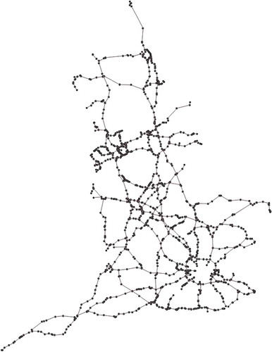
We also test our algorithm on an actual traffic network. The British Government provides the traffic flow data for 15-min intervals on a highway network in England. The network consists of 1000 nodes and 2500 arcs, as shown in Figure 4, and around 240,000 traffic flows (2500 arcs $\times$ 96 time slots) including average travel speed and corresponding journey time are recorded for a day. The dataset is available at https://data.gov.uk/dataset/dft-eng-srn-routes-journey-times.

Figure 4. Highway network in England

For calculating the fuel consumption, we apply the following function developed for a 9.58-ton diesel truck through real-life empirical studies:

$f(v)=871-16.0\times v+0.143\times v^2+32031\times v^{-2}+1.79961\times {10}^{-2}\times 9.58,$

where $f(v)$ is the $\mathrm{C}{\mathrm{O}}_2$ emission rate in g/km and $v$ is speed in km/h. This function is based on the emission model developed by Hickman, Hassel, Joumard, Samaras, and Sorenson (1999) and has been widely used in the related literature (Xiao & Konak, 2016). Note that, by the nature of the proposed approach, there are very few restrictions on the characteristics of the fuel consumption model. The algorithms designed in this paper were implemented using JAVA programming and all experiments which will be described were executed on an Intel i7 2.70 GHz with 16GB of RAM.

5.1. Grid network

We construct 10$\times$10, 20$\times$20, and 30$\times$30 grid networks, where unit distance between adjacent nodes is 5 km. We have three levels for the number of customers, 5, 10, and 20, resulting in nine different problem settings for the test. For each setting, we generate 30 problem instances by randomly allocating customer nodes on the network and arbitrarily determining sequence $\sigma$.

The available speeds of a vehicle are set as integers in a range from 10 km/h to 30 km/h with an increment of 5 km/h based on the average speed of cars and buses in city streets (Ferreira, 2015). Considering the speed range, we use three numbers for ${\tilde{v}}_{ij}^t$ for the minimum weight path algorithm in the approximation scheme, 10, 20, and 30 km/h, resulting in three different paths for a sub-problem. Next, to generate the time-dependent network condition, we determine the interval $[t_1,t_2]$ for each arc $(i,j)\in \mathcal{A}$ by drawing $t_1$ and $t_2$ from uniform distribution $[0,|\mathcal{T}|]$. During the interval, the fuel consumption rate on an arc given a travel speed is multiplied by 110%.

Given sequence $\sigma$ of a problem instance, the time window of customer $d_h$ is computed as $e_{d_h}=e_{d_{h-1}}+\frac{60\times D_{h-1,h}}{V_{max}}-random(0,10)$, and $l_{d_h}=l_{d_{h-1}}+\frac{60\times D_{h-1,h}}{V_{min}}+random(0,10)$, where $V_{max}$ and $V_{min}$ are the maximum and minimum speeds of a vehicle, respectively, and $D_{h-1,h}$ is the shortest distance between customer $h-1$ and $h$. $random(a,b)$ returns a random integer value between $a$ and $b$.

Following the procedures, we generate 270 problem instances and solve them with the proposed approach. Table 1 first shows a summary of the results on the small-sized 10$\times$10 network, where the exact approach can derive an optimal solution to the speed optimization problem within a relatively feasible computation time.

Table 1. Experimental results for 10$\times$10 grid network

			CPU time (sec)
$|{\mathcal{N}}_0|$		Optimality gap^a	Optimal	Approximated
5	avg.	0.14	131.39	0.30
	std.	<0.01	75.94	0.27
	95%Q	0.99	275.96	0.77
	max	1.98	357.17	1.19
10	avg.	0.08	612.35	0.37
	std.	<0.01	202.91	0.17
	95%Q	0.54	96,971	0.68
	max	1.35	1130.03	0.86
20	avg.	0.08	3536.10	0.98
	std.	<0.01	1140.83	0.29
	95%Q	0.46	5367.49	1.51
	max	1.47	6737.34	1.60

^agap: 100 $(\mathrm{\%})$ $\times$ (obj. value obtained by the approximation – obj. value of exact solution)/obj. value of exact soution.

In Table 1, the column ‘Optimality gap’ indicates the quality of the proposed approximation scheme measured as a relative gap of an objective value obtained by the approximation schemes to an optimal objective value. Recall that without applying the approximation schemes described in $\mathcal{\S }$4.3, the proposed approach guarantees the optimality of its solution.

As presented, the optimality gap is not significant and the approximation schemes often find optimal solutions. In addition, the computation time to derive a solution is, remarkably, saved by the approximation schemes: the computation time difference is, on average, a factor of $\approx 440$ for the $|{\mathcal{N}}_0|$=5 instances, but a factor of $\approx 3600$ for $|{\mathcal{N}}_0|$=30 instances. Considering the fact that the optimality gap is, on average, less than 0.14% in the three cases, it is fair to say that the proposed approximation schemes derive near optimal solutions within a short computation time for the speed optimization in relatively small-sized networks.

For the 20$\times$20 and 30$\times$30 networks, we observe that the exact approach cannot derive optimal solutions within a feasible computation time. Therefore, for comparison, instead of referring to optimal solutions, we implement a variant of the approximation scheme that uses the shortest path to a customer in Algorithm 1, which is the practical approach commonly found in the literature on route choice models (Jha, Madanat, & Peeta, 1998). The comparison results for large-scaled networks are summarized in Table 2.

Table 2. Experimental results for large-scaled grid networks

		Network
			20$\times$20		30$\times$30
			gap^a	CPU time (sec)	gap^a	CPU time (sec)
$|{\mathcal{N}}_0|$	5	avg.	20.79	8.76	22.76	36.43
		std.	0.07	10.36	0.06	30.71
		95%Q	30.80	33.69	29.00	95.29
		max	32.97	38.86	36.83	109.56
	10	avg.	21.23	10.57	22.51	32.56
		std.	0.03	14.18	0.04	37.89
		95%Q	26.12	37.07	30.22	96.13
		max	27.00	71.62	31.32	201.64
	20	avg.	20.32	12.18	22.49	52.90
		std.	0.03	4.08	0.02	21.24
		95%Q	24.83	18.82	25.74	82.76
		max	28.95	26.08	27.17	137.03

^agap: (obj. value with the shortest path – obj. value of our solution)/obj. value of our solution × 100 (%).

From Table 2, it can be observed that the approximation scheme deriving a route considering time-dependent travel conditions outperforms the scheme with the shortest path to customers, which neglects the impact of the time-dependent travel conditions. Under our problem setting, 20% of fuel consumption can, on average, be saved by travelling the fuel-efficient route instead of the shortest route. This clearly shows the importance of incorporating routing decisions into the speed optimization problem under the time-dependent travel conditions.

On the other hand, as the size of network increases, the computation time to derive a solution by the proposed algorithm is increased, but still in a reasonable range. This performance opens for near real-time applications of the algorithm in, for example, autonomous systems with AGVs, where routing and speed optimization are conducted in a dynamic manner to respond to frequent system state changes.

5.2. English highway

Next, we test our algorithm using the traffic flow data on the English highway network containing average travel speed and journey time on motorways for every 15-min interval. From a certain traffic flow data for a day (1 August 2014) selected due to completeness of data, a target network is constructed. With the network, three levels for the number of customers, 5, 10, and 20, are considered to generate problem instances.

For a problem instance, we randomly allocate customers to nodes on the network assigning the sequence between them, and specify their time windows in the same manner in the experiments on grid networks. We set $V_{min}$ and $V_{max}$ as 40 km/h and 120 km/h, respectively, considering the speed profile on the traffic flow data. Three speed options, the average speed and the speeds decreased/increased by 10% of the average speed, are put into ${\mathcal{V}}_{ij}^t$. Under the setting, we generate 30 problem instances for each number of customers and derive solutions to the instances.

For comparison, we refer to a solution found by the minimum weight path algorithm (Orda & Rom, 1991) with the average speeds in the flow data. The solution derived by the algorithm represents the best way to minimize the fuel consumption, if a driver drives a vehicle at the average flow speeds of motorways when travelling. This solution is then compared with our own in terms of CO${ }_2$ emission and the total travel time to visit all customers.

To put the results into a practical perspective, we also calculate the total cost for the CO${ }_2$ emission and travel time. Following the experimental setting in Çimen and Soysal (2017), where 1 l of fuel consumption is assumed to generate 2.63 kg of CO${ }_2$, the CO${ }_2$ emission and total travel time are then converted into fuel cost and wage of a driver using the parameters, 1.6€/liter and 0.24€/min, respectively. The comparison results are presented in Table 3.

Table 3. Experimental results for travel on English highway

			Gap
$|{\mathcal{N}}_0|$		CPU time (sec)	CO${ }_2$ emission^a (%)	Travel time^b (%)	$\mathrm{\Delta }{C}^{\hspace{0.17em}}$^c(€)
5	avg.	0.02	17.63	7.26	21.28
	std.	0.01	0.04	0.03	6.93
	0.95Q	0.03	26.47	12.61	32.40
	max	0.05	30.56	16.20	40.48
10	avg.	0.04	18.65	7.91	44.18
	std.	0.01	0.03	0.02	12.36
	0.95Q	0.06	23.92	10.46	59.81
	max	0.06	25.26	14.14	87.45
20	avg.	0.07	16.96	6.74	79.35
	std.	0.02	0.02	0.02	17.19
	0.95Q	0.11	19.32	9.38	108.58
	max	0.10	20.92	9.73	116.38

^aCO${ }_2$ emission: 100($\mathrm{\%}$)$\times$(obj. value by the average speed driving – obj. value of our solution)$/$obj. value of our solution.

^bTravel time: 100($\mathrm{\%}$)$\times$(total travel time of our solution – total travel time by the average speed driving)$/$ total travel time by the average speed driving.

^c$\mathrm{\Delta }C$: Total cost led by the average speed driving – Total cost of our solution.

From Table 3, we see that the proposed algorithm derives solutions in a short time, which is desirable in the context of formulating short-term (e.g. daily) travel schedules. The proposed algorithm also outperforms the minimum weight path algorithm with the average speed in terms of total cost for travel, i.e. sum of fuel cost and drive wage. Specifically, our solutions significantly reduce the CO${ }_2$ emission compared with the solution by the minimum weight path algorithm, whereas our solutions tend to travel longer than the benchmark solutions. Under the cost calculation, the cost saving in CO${ }_2$ emission is greater than the cost increase for the wage, bringing savings in total cost. The cost savings become even more significant as the number of customers increases. These results indicate that the proposed approach enables the provision of fuel-efficient travel plans as well as total cost reduction in realistic transportation scenarios.

6. Discussion

In this section, we examine the factors that lead to performance improvements for the speed optimization problem. Obviously, one of the main factors for the improvement is to address the routing decision that seeks the fuel-(cost)-efficient route considering the time-dependent travel conditions, instead of using a fixed route to customers. The impacts of the routing on the quality of solutions are more comprehensively addressed in $\mathcal{\S }$ 5.

The intermediate nodes, where a vehicle changes its travel speed, also contribute to the performance improvement. Unlike the existing approaches that only have a single speed selection between customer nodes, routes with the intermediate nodes and speeds varying over segments of the route allow us to have sophisticated and advanced transportation schedules bringing reductions in fuel consumption.

From an algorithm perspective, considering multiple routes to customers can contribute to the quality of solutions generated by the proposed approach. Because the algorithms with the approximation schemes restrict the solution space by applying a simplified network constructed by a few routes, the more routes we consider, the larger the solution space will be explored, resulting in better performance. Recall that to minimize the quality loss by the approximation schemes, we generate multiple routes using different values for ${\tilde{v}}_{ij}^t$ in the minimum weight path algorithm.

In fact, our investigation says that, under our problem setting, varying the speed on an arc could not provide the high level of diversity among the routes obtained by the minimum weight path algorithm, while the routes are sufficiently effective to minimize the fuel consumption guaranteeing (near) optimality of the solutions by the routes. The performance improvement by considering multiple routes in the proposed approach is, accordingly, small.

To clearly see the impact of considering multiple routes, we implement the $k$ shortest path algorithm into Algorithm 2 to find routes to a customer and, in turn, construct a simplified network. Please see Yen (1971) for the $k$ shortest path algorithm in detail. This scenario will be relevant to the case when we are also interested in minimizing the travel distance/time of a journey to visit customers.

For a problem setting with the 20$\times$20 grid network and 5 customers, we generate 30 problem instances following the procedures in $\mathcal{\S }$5, and solve the problems using the different $k$ values, $k=1,2,\dots ,5$. We evaluate the performance gap between the solutions found by applying the $k$ shortest paths algorithm and the solutions found by the original approach. Figure 5 shows the results.

Figure 5. Performance improvements by considering more paths

The ‘gap’ in the figure indicates the performance gap. As expected and observed from Figure 5, considering multiple routes in the speed optimization solving has an impact on the quality improvement and this is aligned with the findings in the literature (Garaix et al., 2010; Huang et al., 2017; Liu et al., 2014) and $\mathcal{\S }$ 5.

7. Conclusion

For the speed optimization problem with the time-dependent travel conditions, finding a route considering the time-dependent condition instead of fixing a route in advance can contribute to minimizing fuel consumption. Motivated by this fact, in this study, the speed optimization problem involving the decision-making on both routing to customers and speeds on segments of the routes is addressed.

To solve the problem, algorithms designed based on the shortest path algorithm with the label concept are proposed. Since the algorithms are intractable as the problem size increases, we also propose approximation schemes that sequentially and iteratively solve the routing problem and speed selection on segments of the routes with the limited solution space.

Importantly, the proposed approach is independent of the network structure and the fuel consumption model, which makes it highly generic and applicable to a large number of instances. For example, using a fuel consumption cost for a UAV as a function of its flight speed and a flight network of the UAV, the approach can derive a UAV flight plan, which consists of a route of the unit visiting multiple waypoints and flight speeds over the route, considering time-dependent weather conditions.

Experimental results demonstrate that the proposed approach provides near-optimal solutions within a short computation time, outperforming other benchmark approaches. In particular, the routes found considering time-dependent travel conditions significantly improve the quality of the solution compared with the shortest path, a common practice in transportation services. The transportation cost reduction by the proposed approach is also verified using the traffic flow data on a highway network in England. Based on the performance, a further aspect of the interest includes the use of the solution method for dynamic applications such as re-routing a vehicle in near real-time due to significant changes in environmental and operational conditions and uncertainties on them.

Acknowledgments

The research has been partially supported by the project “Operational Reliability Management System (ORMS)” from Airbus Defence & Space.

Additional information

Funding

This work was supported by the Airbus Defence & Space [N.A].

References

- Armstrong, V. N. (2013). Vessel optimisation for low carbon shipping. Ocean Engineering, 73, 195–207.
- Barth, M., & Boriboonsomsin, K. (2008). Real-world carbon dioxide impacts of traffic congestion. Transportation Research Record: Journal of the Transportation Research Board, 2058(1), 163–171. Los Angeles, CA: SAGE Publications.
- Bektaş, T., & Laporte, G. (2011). The pollution-routing problem. Transportation Research Part B: Methodological, 45(8), 1232–1250.
- Christiansen, M., Fagerholt, K., Nygreen, B., Ronen, D., et al. (2013). Ship routing and scheduling in the new millennium. European Journal of Operational Research, 228(3), 467–483. Elsevier.
- Çimen, M., & Soysal, M. (2017). Time-dependent green vehicle routing problem with stochastic vehicle speeds: An approximate dynamic programming algorithm. Transportation Research Part D: Transport and Environment, 54, 82–98.
- Colomina, I., & Molina, P. (2014). Unmanned aerial systems for photogrammetry and remote sensing: A review. ISPRS Journal of Photogrammetry and Remote Sensing, 92, 79–97.
- Dang, Q.-V., Nielsen, I., Steger-Jensen, K., & Madsen, O. (2014). Scheduling a single mobile robot for part-feeding tasks of production lines. Journal of Intelligent Manufacturing, 25(6), 1271–1287.
- Demir, E., Bektaş, T., & Laporte, G. (2012). An adaptive large neighborhood search heuristic for the pollution-routing problem. European Journal of Operational Research, 223(2), 346–359.
- Dorling, K., Heinrichs, J., Messier, G. G., & Magierowski, S. (2017). Vehicle routing problems for drone delivery. IEEE Transactions on Systems, Man, and Cybernetics: Systems, 47(1), 70–85.
- Fagerholt, K. (2001). Ship scheduling with soft time windows: An optimisation based approach. European Journal of Operational Research, 131(3), 559–571.
- Fagerholt, K., Laporte, G., & Norstad, I. (2010). Reducing fuel emissions by optimizing speed on shipping routes. Journal of the Operational Research Society, 61(3), 523–529.
- Ferreira, E. A. (2015). The concept of effective speed. Urban Independence. Retrieved from https://www.bikecitizens.net/the-concept-of-effective-speed/
- Franceschetti, A., Honhon, D., Laporte, G., & Van Woensel, T. (2018). A shortest-path algorithm for the departure time and speed optimization problem. Transportation Science, 52(4), 756–768. INFORMS.
- Franceschetti, A., Honhon, D., Van Woensel, T., Bektaş, T., & Laporte, G. (2013). The time-dependent pollution-routing problem. Transportation Research Part B: Methodological, 56, 265–293.
- Garaix, T., Artigues, C., Feillet, D., & Josselin, D. (2010). Vehicle routing problems with alternative paths: An application to on-demand transportation. European Journal of Operational Research, 204(1), 62–75.
- Hickman, J., Hassel, D., Joumard, R., Samaras, Z., & Sorenson, S. (1999). Methodology for calculating transport emissions and energy consumption.
- Huang, Y., Zhao, L., Van Woensel, T., & Gross, J.-P. (2017). Time-dependent vehicle routing problem with path flexibility. Transportation Research Part B: Methodological, 95, 169–195.
- Hvattum, L. M., Norstad, I., Fagerholt, K., & Laporte, G. (2013). Analysis of an exact algorithm for the vessel speed optimization problem. Networks, 62(2), 132–135.
- Jabali, O., Woensel, T., & de Kok, A. (2012). Analysis of travel times and co2 emissions in time-dependent vehicle routing. Production and Operations Management, 21(6), 1060–1074.
- Jha, M., Madanat, S., & Peeta, S. (1998). Perception updating and day-to-day travel choice dynamics in traffic networks with information provision. Transportation Research Part C: Emerging Technologies, 6(3), 189–212.
- Kramer, R., Maculan, N., Subramanian, A., & Vidal, T. (2015a). A speed and departure time optimization algorithm for the pollution-routing problem. European Journal of Operational Research, 247(3), 782–787.
- Kramer, R., Subramanian, A., Vidal, T., & Lucdio Dos Anjos, F. C. (2015b). A matheuristic approach for the pollution-routing problem. European Journal of Operational Research, 243(2), 523–539.
- Lin, C., Choy, K. L., Ho, G. T., Chung, S. H., & Lam, H. (2014). Survey of green vehicle routing problem: Past and future trends. Expert Systems with Applications, 41(4), 1118–1138.
- Lindstad, H., Asbjørnslett, B. E., & Jullumstrø, E. (2013). Assessment of profit, cost and emissions by varying speed as a function of sea conditions and freight market. Transportation Research Part D: Transport and Environment, 19, 5–12.
- Liu, W.-Y., Lin, -C.-C., Chiu, C.-R., Tsao, Y.-S., & Wang, Q. (2014). Minimizing the carbon footprint for the time-dependent heterogeneous-fleet vehicle routing problem with alternative paths. Sustainability, 6(7), 4658–4684.
- Malandraki, C., & Daskin, M. S. (1992). Time dependent vehicle routing problems: Formulations, properties and heuristic algorithms. Transportation Science, 26(3), 185–200.
- Nielsen, I., Dang, Q.-V., Bocewicz, G., & Banaszak, Z. (2017). A methodology for implementation of mobile robot in adaptive manufacturing environments. Journal of Intelligent Manufacturing, 28(5), 1171–1188.
- Norstad, I., Fagerholt, K., & Laporte, G. (2011). Tramp ship routing and scheduling with speed optimization. Transportation Research Part C: Emerging Technologies, 19(5), 853–865.
- Orda, A., & Rom, R. (1991). Minimum weight paths in time-dependent networks. Networks, 21(3), 295–319.
- Psaraftis, H. N., & Kontovas, C. A. (2014). Ship speed optimization: Concepts, models and combined speed-routing scenarios. Transportation Research Part C: Emerging Technologies, 44, 52–69.
- Qian, J., & Eglese, R. (2014). Finding least fuel emission paths in a network with time-varying speeds. Networks, 63(1), 96–106.
- Qian, J., & Eglese, R. (2016). Fuel emissions optimization in vehicle routing problems with time-varying speeds. European Journal of Operational Research, 248(3), 840–848.
- Tseng, C.-M., Chau, C.-K., Elbassioni, K., & Khonji, M. (2017). Flight tour planning with recharging optimization for battery-operated autonomous drones. arXiv Preprint, arXiv, 1703.10049.
- Xiao, Y., & Konak, A. (2016). The heterogeneous green vehicle routing and scheduling problem with time-varying traffic congestion. Transportation Research Part E: Logistics and Transportation Review, 88, 146–166.
- Yen, J. Y. (1971). Finding the k shortest loopless paths in a network. Management Science, 17(11), 712–716.