Optimal inventory replenishment and shipment policies in a four-echelon supply chain for growing items with imperfect quality

ABSTRACT

Quality control is an important consideration in food production systems which often start with farming and processing operations and finish with consumption. This study develops an integrated inventory control model for a four-echelon supply chain (with farming, processing, screening and retail operations). The farmer grows newborn items and then delivers them to a processor once the items are mature enough. At the processing plant, the items are slaughtered, processed, packaged and screened for quality. The processor then delivers a certain number of equally sized batches of good quality processed inventory to the retailer who satisfies customer demand for good quality processed inventory. The processor sells the processed poorer quality inventory at a discounted price and as a single batch to secondary markets. The proposed supply chain inventory system is formulated as a profit maximisation problem with the number of batches of good quality processed inventory and the order quantity as the decision variables.

KEYWORDS:

• Joint economic lot size
• growing items
• imperfect quality
• inventory management
• four-echelon supply chain

1. Introduction

1.1. Context

Building upon Rezaei (2014) ’s economic order quantity (EOQ) model for growing items, Sebatjane and Adetunji (2019a) developed an extension which incorporated imperfect quality. This extension captures some aspects of realistic food production systems, particularly item growth and the presence of items that are of inferior quality. Nonetheless, the model falls short of being an accurate representation of a real-life inventory system because of some of the assumptions made when it was being developed, three of which are addressed in this paper. The first assumption is that immediately after the items have grown to the target weight, they are slaughtered and sold to market instantly and the second one is that all the newborn items survive throughout the growing cycle. The third assumption is that one entity is responsible for all the activities, this is not always the case, especially in today’s business environment where the benefits of supply chain management are documented. Consequently, multiple entities are involved in getting the slaughtered product to market, albeit at different stages. While these assumptions simplify the modelling process, they are unrealistic because there is usually some form of processing prior to selling the items to end consumers and growing items, which are living organisms, are not immune to mortality.

To overcome some of the shortcomings in Sebatjane and Adetunji (2019a) ’s model, an integrated multi-echelon supply chain is suggested. The proposed supply chain consists of three members (i.e. a farmer, a processor and a retailer) and four echelons (i.e. farming, processing, screening and selling). The farmer, who receives the items as newborns at the beginning of a replenishment cycle, is responsible for growing the items provided that some of the items do not survive to the end of the growing period due to mortality. The processor is involved in the transformation of the fully grown live items into saleable items through slaughtering, preparation and packaging (collectively termed processing), while the retailer sells the processed items to end users. Prior to sending the processed items to the retailer, the processor screens them for quality to ensure that consumers get them in the correct form (from a consumer health and safety perspective).

1.2. Objectives

The main objective of this paper is to formulate a coordinated model for managing inventory in a supply chain with growing items while taking into account item mortality and quality control initiatives. In addition to the main objective, the paper has a few sub-objectives that are aimed at investigating, through numerical experimentation, the effects of item mortality during the farming stage, the presence of imperfect quality inventory after processing and the adopted shipment policy between the processor and the retailer on the supply chain’s profit and ordering policy.

1.3. Relevance

The presence of illnesses, pests (in the case of crops) and predators (in the case of livestock) makes item mortality an important factor to consider when studying inventory systems with growing items. In reality, not all the newborn items ordered when a replenishment cycle starts to make it to the processing stage due to mortality.

The primary source of most consumable food products is growing items. However, these items are rarely consumed in their original form. The items go through a number of stages before they are in a form suitable for consumption. These stages represent supply chain echelons and in the context of this article, four are identified, namely, farming, processing, screening and selling. This paper uses this fact to propose a model for inventory control in a four-echelon supply chain for growing items when there is a possibility of having inferior quality items. For this reason, government regulations require food items to be checked for quality before they are sold to consumers in order to ensure that the health and safety of consumers are not compromised.

Given that growing items were only incorporated in inventory theory recently (Rezaei, 2014), it appears that no study has considered an integrated inventory control system for growing items in a four-echelon supply chain with item processing considering mortality (in the case live items) and quality (in the case of processed items). This study is aimed at filling this void in the literature. The model and results from the numerical analysis can be used as a guideline for managers in charge of making purchasing decisions in industries involved in the broader food chain.

1.4. Organisation

Besides the introductory section, this paper has five other sections. A review of relevant articles in the literature is provided in Section 2. In addition to providing a description of the proposed inventory control system, Section 3 also lists the assumptions and notations used when formulating the model. The model is then developed in Section 4. Following this, important managerial insights are drawn from a numerical example presented in Section 5 and then concluding remarks are given in Section 6.

2. Literature review

2.1. Growing inventory items

The concept of item growth was incorporated by Rezaei (2014) to inventory theory through the development of an EOQ-type inventory control model for items that can grow. In the context of Rezaei (2014) ’s model, item growth was only quantified by an increase in weight (i.e. the difference between growing and conventional items is that growing items experience an increase in weight during the course of the replenishment cycle). It was assumed that the items are allowed to grow until maturity, following which they are slaughtered and sold to meet consumer demand. The model was essentially an extension of Harris (1913) ’s work, developed by relaxing the implicit assumption that the weight of the item remains constant throughout the replenishment cycle.

Rezaei (2014) ’s work has received attention from numerous researchers who have extended the model to suit various practical situations. Nobil et al. (2019) proposed an inventory control model for growing items for a situation with permissible shortages that are fully backordered. Sebatjane and Adetunji (2019a) extended the model to a case where a percentage of the slaughtered inventory is of poorer quality. Khalilpourazari and Pasandideh (2019) studied a multi-item inventory control system for growing items taking in to account budget and warehouse capacity constraints. Quantity discounts, specifically marginal quantity discounts, were incorporated through Sebatjane and Adetunji (2019b) ’s work. Malekitabar et al. (2019) developed an inventory control model for growing-mortal items in a supply chain with revenue- and cost-sharing contracts in place through a case study for trout fish production. Sebatjane and Adetunji (2019c) formulated a model for managing growing inventory items in a three-level supply with separate farming, processing and retail operations.

2.2. Integrated inventory systems with imperfect quality items

2.2.1. Integrated inventory systems

The idea of a multi-echelon inventory system was introduced by Clark and Scarf (1960) who considered a system with a wholesaler and a retailer aimed at reducing the joint total cost. Goyal (1977) extended the idea to a more generalised inventory system and consequently developed one of the earliest integrated inventory systems, which consisted of a single vendor and a single buyer. It was assumed that the vendor does not produce any of the items, but rather acts as a distributor and for that reason, the vendor had an unlimited replenishment rate. The buyer was assumed to receive equally sized shipments of items from the vendor. The model was aimed at determining the optimal shipment size from the vendor to the buyer which minimises total system costs. Banerjee (1986) presented a variation of the model which considered a vendor who produces the items on a lot-for-lot basis.

2.2.2. Inventory items with imperfect quality items

Item quality was incorporated to inventory management research by Salameh and Jaber (2000) through relaxing the implicit assumption made in most inventory models that all the items received in each order are of good quality. The authors proposed an inventory situation in which a specific percentage of the ordered items is of inferior quality. Before the items are sold, they are all subjected to a screening process in order to isolate the good quality items from those of poorer quality. A simpler method, with minimal effects on the expected total profit, for computing the EOQ in Salameh and Jaber (2000) ’s model was proposed by Goyal and Cardenas-Barron (2002). Cardenas-Barron (2000) and Maddah and Jaber (2008) rectified computational mistakes made in Salameh and Jaber (2000) ’s model pertaining to the EOQ and the expected total profit functions.

2.2.3. Integrated inventory systems with imperfect quality items

Imperfect quality was first considered in integrated inventory systems by Huang (2003) through extending Salameh and Jaber (2000) ’s work to a supply chain with a vendor who produces items and a buyer who screens them for quality. Based upon Goyal and Cardenas-Barron (2002) ’s correction of Salameh and Jaber (2000) ’s model, Goyal et al. (2003) corrected the earlier integrated inventory control model for imperfect quality items proposed by Huang (2003). The models proposed by Huang (2003) and Goyal et al. (2003) were formulated under the assumption that the percentage of poorer quality items is random, Ouyang et al. (2006) deviated from this assumption and developed a model under the assumption that the poorer quality fraction is a triangular fuzzy number. Konstantaras et al. (2007) considered a version of the EOQ model for items with imperfect quality in a system where the items are inspected in-house at a secondary warehouse. Glock and Tan (2011) relaxed the single buyer-single vendor assumption made in most models and developed one with a single buyer and multiple vendors. Kreng (2011) developed an extension which considered two-way trade-credit financing (i.e. the vendor offers the buyer a grace period to settle the bill and the buyer also offers a grace period to consumers). Hsu and Hsu (2013) extended Goyal et al. (2003) ’s model to a case with permissible (and fully backordered) shortages. Khan et al. (2014) studied an integrated inventory control system with imperfect quality items by taking the effects of two human factors, namely, learning in production (i.e. production efficiency improves from one production cycle to the next because of the experience the operators get) and errors in inspection (i.e. the inspectors can make mistakes during the screening process), into consideration. The recent emphasis on green supply chain management motivated Zanoni et al. (2014) to formulate a model for a two-echelon supply chain where the demand is a function of both the selling price and the environmental performance of the supply chain. Khan et al. (2016) developed a coordinated inventory control model for items with inferior quality for a vendor and a buyer in a supply chain where the vendor has the responsibility of managing the inventory at the buyer’s facility. Jauhari and Saga (2017) developed an extension of the integrated vendor-buyer inventory control system with imperfect quality items by considering the demand rate to be stochastic, the ordering cost to be fuzzy and the (vendor’s) production rate to be flexible. Castellano et al. (2017) studied an inventory control system with quality considerations, price discounts based on permitted shortages, stochastic demand and controllable lead time under a periodic review policy. Tiwari et al. (2018) proposed an inventory control model for a vendor and a buyer producing and selling, respectively, deteriorating items with both environmental and quality considerations.

2.3. Research gap and contribution

Table 1 provides a comparison of previous studies on inventory control for integrated production inventory system with and without imperfect quality and inventory control for growing items. In addition to highlighting the contributions made by various researchers, the comparison also shows the research gap identified in literature. The table gives the impression that no published inventory control model for growing items has considered a four-echelon integrated supply chain system with mortality and quality considerations. This study is the first attempt at developing a coordinated model for managing growing inventory items in a system with farming, processing, screening and retail operations while taking into account the possibility of having poorer quality items and possible growth mortality. The proposed inventory system is reminiscent of most food production chains which consist of multiple parties involved at different stages of food production where quality control is a very important consideration given the potential implications on consumers’ health if poorer quality items are sold.

Table 1. Contribution and gap analysis of similar inventory models in literature

	Types of items		Imperfect	Integrated	Additional
	Conventional	Growing	quality	inventory	inventory system
References	items	items	system	system	characteristics
Clark and Scarf (1960)	✓			✓
Goyal (1977)	✓			✓
Banerjee (1986)	✓			✓	Lot-for-lot policy
Salameh and Jaber (2000)	✓		✓
Cardenas-Barron (2000)	✓		✓
Huang (2003)	✓		✓	✓
Ouyang et al. (2006)	✓		✓	✓	Fuzzy theory
Konstantaras et al. (2007)	✓		✓		In-house screening
Maddah and Jaber (2008)	✓		✓
Glock and Tan (2011)	✓		✓	✓	Multiple vendors
Kreng (2011)	✓		✓	✓	Trade credit
Hsu and Hsu (2013)	✓		✓	✓	Shortages
Khan et al. (2014)	✓		✓	✓	Screening errors
Rezaei (2014)		✓
Khan et al. (2016)	✓		✓	✓	Consignment stock
Jauhari and Saga (2017)	✓		✓	✓	Stochastic demand
Tiwari et al. (2018)	✓		✓	✓	Carbon emissions
Khalilpourazari and Pasandideh (2019)		✓			Multiple items
Malekitabar et al. (2019)		✓		✓	Revenue sharing
Nobil et al. (2019)		✓			Shortages
Sebatjane and Adetunji (2019a)		✓	✓
Sebatjane and Adetunji (2019b)		✓			Quantity discounts
This study		✓	✓	✓	Item mortality

3. Problem description

The inventory problem at hand considers a four-echelon supply chain for growing items with the farming, processing, screening and retail operations as the echelons. The farmer is responsible for growing the items which are received as newborns. The fully grown items are then instantaneously shipped to the processor for transformation into a saleable form. The items are deemed fully grown or mature once they grow to a specified weight. The processing stage is not perfect and it thus produces some items of poorer quality, in addition to those of good quality. As a way of ensuring that the health and safety of end users are not compromised, the processor is also responsible for quality control (in addition to processing the items) and for this reason, the processor has two facilities, one for processing and the other one for quality screening. Throughout the screening process, the processor delivers an integer number of batches of good quality processed inventory to the retailer who meets consumer demand for good quality processed inventory. The processed poorer quality inventory is accumulated throughout the screening process and is then sold as a single batch to secondary markets when the screening process ends.

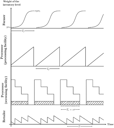
The inventory system profile for the problem at hand is depicted in Figure 1. For the farmer’s inventory profile, the weight depicted in the graph is that of the live items as they grow throughout the cycle. In the case of the processor’s and the retailer’s inventory profiles, the graph shows the changes that occur to the processed inventory. At the processing facility, live items are transformed into saleable processed items and the weight of the processed inventory increases gradually at a certain rate. At the screening warehouse, the processed inventory is inspected for quality and batches of good quality are transferred to the retailer while the poorer quality processed inventory (shown as the shaded portion in the figure) accumulates at the warehouse. The processed poorer quality inventory is then sold off as a single batch when screening ends.

Figure 1. Inventory system profile for a farmer, a processor and a retailer in a supply chain for growing items with imperfect processing (with $n=3$ for illustrative purposes)

The following notations are employed when modelling the proposed supply chain inventory system:

D Demand rate for good quality processed items in weight units per unit time

R Processing rate in weight units per unit time

w(t)The weight of an item at time $t$

w₀ Newborn weight of each item

w₁Maturity (i.e. target) weight of each item

yFarmer’s order quantity for live newborn items per cycle

xFraction of the live items which survive throughout the growth period

p_v Procurement (or purchasing) cost per weight unit of live newborn item

K_fFarmer’s setup cost per cycle

c_fFarmer’s feeding cost per weight unit (of live inventory) per unit time

m_f Farmer’s mortality cost per weight unit (of dead inventory) per unit time

T_fDuration of the farmer’s growth period

p_fFarmer’s selling price per weight unit of live items

K_pProcessor’s processing facility setup cost per cycle

h_pProcessor’s processing facility holding cost per weight unit per unit time

T_p Time required to process the entire lot size

K_sProcessor’s cost of sending a single batch of good quality processed inventory to the retailer (from the screening facility)

h_s Processor’s screening facility holding cost per weight unit per unit time

$\tau$ Time between consecutive deliveries of good quality batches from the screening facility to the retailer

n Number of batches of good quality processed inventory delivered to the retailer during a single screening run

T_sTime required to screen the entire lot size

p_pProcessor’s selling price per weight unit of good quality inventory

p_qProcessor’s selling price per weight unit of poorer quality inventory

a Fraction of processed inventory that are of poorer quality

s Screening rate in weight units per unit time

l Screening cost per weight unit

z Number of items per batch of good quality processed items sent (by the processor) to the retailer

T Replenishment cycle time for all echelons (defined, from Figure 1, as successive moments when the retailer’s processed inventory reaches zero)

K_rRetailer’s ordering cost per cycle

h_rRetailer’s holding cost per weight unit per unit time

p_rRetailer’s selling price per weight unit of good quality processed inventory

$\alpha$The items’ asymptotic weight

$\beta$Constant of integration

$\lambda$Exponential growth rate of the items

A number of assumptions are made in order to model the proposed supply chain inventory system. These include

• There is only one farmer, one processor and one retailer in the supply chain involved, respectively, in the growing, the processing with screening and the selling of a single type of item.

• A fraction of the live inventory items does not survive until the end of the growth period.

• The processor’s processing rate is greater than the retailer’s demand rate and both quantities are deterministic constants.

• A fraction of the processed inventory does not meet the required quality standard.

• As soon as processing is complete, the entire processed lot is transferred to a screening warehouse where a 100% screening process takes place in which the items are classified as either being of good quality or poorer quality.

• The screening rate is greater than the demand rate.

• During the screening process, equally sized batches of good quality processed inventory are sent to the retailer.

• The retailer uses the good quality processed inventory to meet consumer demand as soon as the first batch is delivered.

• The poorer quality processed inventory are allowed to accumulate at the processor’s screening warehouse from where they are sold when a single screening run ends.

• Poorer quality processed items can not be reworked.

• Holding costs are incurred only for the ready-to-consume (i.e. processed) items.

• The retailer’s holding costs are higher than those of the processor due to value adding as the items move downstream in the supply chain.

• Order lead time is zero and shortages are not permitted.

4. Model formulation

4.1. Farmer’s profit

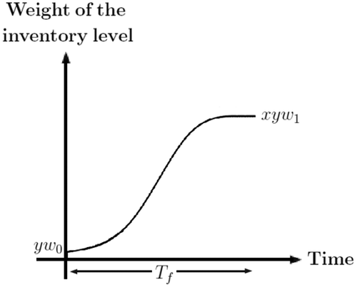
Figure 2 depicts the weight of the farmer’s live inventory throughout the growth period. As the items are fed, their weight increases gradually from an initial newborn weight of $w_0$ to a target maturity weight of $w_1$ at the end of the growing period (of duration $T_f$).

Figure 2. The farmer’s inventory system profile

The farmer’s replenishment cycle starts with the placement of an order for $y$ live newborn items. The farmer procures live newborn items from a vendor who charges $p_v$ per weight unit of the newborn items. Given that at the time of purchase the weight of each item is $w_0$, the farmer’s purchase cost per cycle, $P{C}_f$, is therefore

(1) $P{C}_f=p_{v}y{w}_0.$(1)

There is a fixed cost of $K_f$ associated with setting up for a new growing cycle. The farmer’s setup cost per cycle, $K{C}_f$, is therefore

(2) $K{C}_f=K_f.$(2)

The items are allowed to grow until their weight reaches a certain target (i.e. the maturity weight $w_1$). At that point, they are delivered to the processor for processing and screening. Due to its ‘S’-shaped curve, the logistic function is used to model the items’ growth function, given by

(3) $w(t)=\frac{\alpha }{1+\beta e^{-\lambda t}}.$(3)

When the farmer’s growth period ends, the weight of the surviving items would have reached the target weight of $w_1$. From Equation (3)(3) $w(t)=\frac{\alpha }{1+\beta e^{-\lambda t}}.$(3) , the length of the growth period, $T_f$, is computed using the target maturity weight as

(4) $T_f=-\frac{ln\left[\frac{1}{\beta }\left(\frac{\alpha }{w_1}-1\right)\right]}{\lambda }.$(4)

The farmer’s cyclic feeding cost, $F{C}_f$, computed by multiplying the feeding cost per weight unit ($c_f$), the fraction of items which survive ($x$), and the area under the graph showing the items’ growth trajectory (as given in Figure 2) are given by

(5) $F{C}_f=c_{f}x{\int }_0^{T_f}yw(t)dt=c_{f}xy\left\{\alpha T_f+\frac{\alpha }{\lambda }\left[ln\left(1+\beta e^{-\lambda T_f}\right)-ln(1+\beta )\right]\right\}.$(5)

The farmer incurs a cost associated with disposing the fraction of newborn items which do not survive until the end of the growing cycle. The farmer’s mortality cost cycle, $M{C}_f$, is determined as the product of the farmer’s average inventory level (i.e the area under the graph of the farmer’s inventory system profile), the fraction of items which do not survive ($1-x$) and the mortality cost per weight unit per unit time ($m_f$). Hence,

(6) $M{C}_f=m_f(1-x){\int }_0^{T_f}yw(t)dt=m_f(1-x)y\left\{\alpha T_f+\frac{\alpha }{\lambda }\left[ln\left(1+\beta e^{-\lambda T_f}\right)-ln(1+\beta )\right]\right\}.$(6)

Since the items have a survival rate of $x$, when the farmer’s replenishment cycle ends, the weight of all the surviving items would be given by $xy{w}_1$. This lot is then transferred to the processor for further processing and screening. The weight $xy{w}_1$ represents the processor’s lot size. The farmer charges the processor $p_f$ for each weight unit of the surviving live inventory. The farmer’s revenue per cycle, $T{R}_f$, is therefore

(7) $T{R}_f=p_{f}xy{w}_1.$(7)

The farmer’s total profit per cycle, $T{P}_f$, is the farmer’s cyclic revenue [i.e. Equation (7)(7) $T{R}_f=p_{f}xy{w}_1.$(7) ] less the farmer’s cyclic total costs [i.e the sum of Equations (1)(1) $P{C}_f=p_{v}y{w}_0.$(1) , (2(2) $K{C}_f=K_f.$(2) ), (5(5) $F{C}_f=c_{f}x{\int }_0^{T_f}yw(t)dt=c_{f}xy\left\{\alpha T_f+\frac{\alpha }{\lambda }\left[ln\left(1+\beta e^{-\lambda T_f}\right)-ln(1+\beta )\right]\right\}.$(5) ) and (6(6) $M{C}_f=m_f(1-x){\int }_0^{T_f}yw(t)dt=m_f(1-x)y\left\{\alpha T_f+\frac{\alpha }{\lambda }\left[ln\left(1+\beta e^{-\lambda T_f}\right)-ln(1+\beta )\right]\right\}.$(6) )] and it is given by

(8) $T{P}_f=p_{f}xy{w}_1-p_{v}y{w}_0-K_f-y\left\{\alpha T_f+\frac{\alpha }{\lambda }\left[ln\left(1+\beta e^{-\lambda T_f}\right)-ln(1+\beta )\right]\right\}\left[c_{f}x+m_f(1-x)\right].$(8)

4.2. Processor’s profit

4.2.1. Processor’s processing facility

The inventory system profile for processed inventory in the processing facility, depicted in Figure 3, is used to determine various components of the costs incurred in the processing facility. The weight of the processed inventory increases at a processing rate of $R$ as the processor transforms the live items (received from the farmer) into saleable processed items.

Figure 3. Inventory system profile for the processor’s processing facility

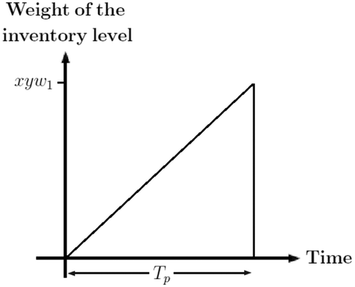
The entire lot size received from the farmer (i.e. $xy{w}_1$) is processed at a rate $R$. This means that the duration of the processing period is

(9) $T_p=\frac{xy{w}_1}{R}.$(9)

The processor incurs a fixed cost of $K_p$ at the start of each processing run and therefore the setup cost per cycle, $K{C}_p$, is

(10) $K{C}_p=K_p.$(10)

The processor procures fully grown live items from the farmer for processing. Given that the farmer charges $p_f$ per weight unit of inventory, the processor’s procurement cost per cycle, $P{C}_p$, is

(11) $P{C}_p=p_{f}xy{w}_1.$(11)

The holding cost per cycle at the processing facility, $H{C}_p$, is computed by multiplying the holding cost per weight unit in the facility, $h_p$, by the area under the inventory system graph, as given in Figure 3, and it is given by

(12) $H{C}_p=h_p\left(\frac{x^2{y}^2{w}_1^2}{2R}\right).$(12)

The total cost (per cycle) at the processing facility, $T{C}_p$, is determined by adding Equations (10)(10) $K{C}_p=K_p.$(10) , (11(11) $P{C}_p=p_{f}xy{w}_1.$(11) ) and (12(12) $H{C}_p=h_p\left(\frac{x^2{y}^2{w}_1^2}{2R}\right).$(12) ), resulting in

(13) $T{C}_p=K_p+p_{f}xy{w}_1+h_p\left(\frac{x^2{y}^2{w}_1^2}{2R}\right).$(13)

4.2.2. Processor’s screening facility

Once the entire lot is processed, it is transferred to a screening warehouse for quality control. In the screening warehouse, the processor incurs holding, screening and transfer costs. Figure 4 depicts the changes to the weight of the processed inventory in the screening warehouse. A fraction, $a$, of the processed inventory does not meet the required quality standard (i.e these inventory items are of poorer quality). This means that the weight of good quality processed inventory is $xy{w}_1(1-a)$, and from this the processor ships $n$ batches (each weighing $z{w}_1$) to the retailer at equally spaced time intervals.

Figure 4. Inventory system profile for the processor’s screening facility (with $n=3$ for illustrative purposes)

Since the processor screens the entire lot they received from the farmer (i.e. $xy{w}_1$) for quality at a rate of $s$, the duration of the screening period, $T_s$, is thus

(14) $T_s=\frac{xy{w}_1}{s}.$(14)

At equally spaced time intervals of $\tau$, the processor delivers an integer number of shipments ($n$ in this case) of good quality processed inventory to the retailer. Therefore, the duration of the time interval between successive deliveries of good quality items is

(15) $\tau =\frac{xy{w}_1}{ns}.$(15)

In each screening run, the weight of items of good quality that the processor has is $xy{w}_1(1-a)$. From this, the processor delivers $n$ batches of good quality processed inventory, each batch being of size $z{w}_1$, to the retailer. The weight of each batch of good quality processed inventory is thus

(16) $z{w}_1=\frac{xy{w}_1(1-a)}{n}.$(16)

The processor also incurs a fixed cost for sending a batch of good quality processed inventory to the retailer. Since the processor sends $n$ batches to the retailer during a single screening run, the transfer cost per cycle, $K{C}_s$, is thus

(17) $K{C}_s=n{K}_s.$(17)

The entire lot is subjected to quality screening process in order to separate the items. The processor incurs a cost of $l$ per weight unit of the processed inventory screened. Therefore, the processor’s screening cost per cycle, $L{C}_s$, is

(18) $L{C}_s=lxy{w}_1.$(18)

The holding cost per cycle at the screening warehouse, $H{C}_s$, is computed by multiplying the holding cost per weight unit by the area under the graph depicting the processed inventory system profile as given in Figure 4. It follows that

(19) $H{C}_s=h_s\left[\frac{x^2{y}^2{w}_1^2}{s}-\frac{(n-1)x^2{y}^2{w}_1^2(1-a)}{2ns}\right].$(19)

The cyclic total cost incurred by the processor at the screening warehouse ($T{C}_s$), computed by summing Equations (17)(17) $K{C}_s=n{K}_s.$(17) , (18(18) $L{C}_s=lxy{w}_1.$(18) ) and (19(19) $H{C}_s=h_s\left[\frac{x^2{y}^2{w}_1^2}{s}-\frac{(n-1)x^2{y}^2{w}_1^2(1-a)}{2ns}\right].$(19) ), is therefore

(20) $T{C}_s=n{K}_s+lxy{w}_1+h_s\left[\frac{x^2{y}^2{w}_1^2}{s}-\frac{(n-1)x^2{y}^2{w}_1^2(1-a)}{2ns}\right].$(20)

The processor delivers $n$ batches of good quality items to the retailer with each batch weighing $z{w}_1$. Noting that all the batches delivered during a single processing cycle have a combined weight of $xy{w}_1(1-a)$ and that the processor charges the retailer $p_p$ per weight unit of good quality processed inventory, the processor’s cyclic revenue from good quality processed inventory, $T{R}_p$, is thus

(21) $T{R}_p=p_{p}xy{w}_1(1-a).$(21)

After the screening process, the processor sells the poorer quality processed inventory at a cost of $p_q$ per weight unit to secondary markets in a single batch. This means that the processor’s cyclic revenue from sales of poorer quality processed inventory, $T{R}_q$, is

(22) $T{R}_q=p_{q}xy{w}_{1}a.$(22)

The processor’s cyclic profit, $T{P}_p$, is computed as the revenue from both good and poorer quality inventory [i.e the sum of Equations (21)(21) $T{R}_p=p_{p}xy{w}_1(1-a).$(21) and (22(22) $T{R}_q=p_{q}xy{w}_{1}a.$(22) )] less the total cost [i.e the sum of Equations (13)(13) $T{C}_p=K_p+p_{f}xy{w}_1+h_p\left(\frac{x^2{y}^2{w}_1^2}{2R}\right).$(13) and (20(20) $T{C}_s=n{K}_s+lxy{w}_1+h_s\left[\frac{x^2{y}^2{w}_1^2}{s}-\frac{(n-1)x^2{y}^2{w}_1^2(1-a)}{2ns}\right].$(20) )] and is thus

$T{P}_p=p_{p}xy{w}_1(1-a)+p_{q}xy{w}_{1}a-K_p-p_{f}xy{w}_1-h_p\left(\frac{x^2{y}^2{w}_1^2}{2R}\right)-n{K}_s-lxy{w}_1$

(23) $-h_s\left[\frac{x^2{y}^2{w}_1^2}{s}-\frac{(n-1)x^2{y}^2{w}_1^2(1-a)}{2ns}\right].$(23)

4.3. Retailer’s profit

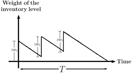
Figure 5 shows the behaviour of the retailer’s processed inventory level over time. The retailer faces a demand rate (for good quality processed inventory) of $D$. To meet this demand, the retailer receives $n$ batches of size $z{w}_1$ from the processor after the items have been screened for quality. Altogether, these batches add up to $xy{w}_1(1-a)$ between successive order cycles (i.e. when the retailer’s inventory level reaches zero). The duration of time between successive order cycles is therefore

(24) $T=\frac{xy{w}_1(1-a)}{D}.$(24)

Figure 5. The retailer’s inventory system profile (with $n=3$ for illustrative purposes)

A fixed ordering cost of $K_r$ is incurred whenever the retailer places an order of $xy{w}_1(1-a)$ good quality items (received in $n$ batches of $z{w}_1$). The retailer’s cyclic ordering cost, $K{C}_r$, is thus

(25) $K{C}_r=K_r$(25)

The retailer procures processed good quality inventory from the processor at a cost of $p_p$ per weight unit. Given that the retailer procures good quality inventory weighing $xy{w}_1(1-a)$ per cycle, their (the retailer’s) procurement cost per cycle, $P{C}_r$, is

(26) $P{C}_r=p_{p}xy{w}_1(1-a).$(26)

Figure 6, a redrawn version of Figure 5, is utilised to determine the area under the graph of the retailer’s processed inventory level (in weight units). The redrawn version makes the computation of the area easier and the method is adopted from Konstantaras et al. (2007). This area is computed by subtracting the area of $n(n-1)/2$ parallelograms of type ABCD from the area of triangle DEF. It follows that

(27) $\begin{array}{cc}\mathrm{A}\mathrm{r}\mathrm{e}{\mathrm{a}}_r& =[\mathrm{A}\mathrm{r}\mathrm{e}\mathrm{a}\mathrm{o}\mathrm{f}\mathrm{t}\mathrm{r}\mathrm{i}\mathrm{a}\mathrm{n}\mathrm{g}\mathrm{l}\mathrm{e}\mathrm{D}\mathrm{E}\mathrm{F}]-\left[\frac{n(n-1)}{2}(\mathrm{A}\mathrm{r}\mathrm{e}\mathrm{a}\mathrm{o}\mathrm{f}\mathrm{p}\mathrm{a}\mathrm{r}\mathrm{a}\mathrm{l}\mathrm{l}\mathrm{e}\mathrm{l}\mathrm{o}\mathrm{g}\mathrm{r}\mathrm{a}\mathrm{m}\mathrm{A}\mathrm{B}\mathrm{C}\mathrm{D})\right]\\ \hspace{0.17em}& =\left[\frac{xy{w}_1(1-a)T}{2}\right]-\left[\frac{n(n-1)z{w}_1\tau }{2}\right]\\ \hspace{0.17em}& =\left[\frac{xy{w}_1(1-a)T}{2}-\frac{(n-1)x^2{y}^2{w}_1^2(1-a)}{2ns}\right].\end{array}$(27)

Figure 6. Redrawn version of the retailer’s inventory system profile (with $n=3$ for illustrative purposes)[modified from Konstantaras et al. (2007)]

This area is multiplied with the holding cost per weight unit to determine the holding cost incurred by the retailer in each cycle, $H{C}_r$, as

(28) $H{C}_r=h_r\left[\frac{xy{w}_1(1-a)T}{2}-\frac{(n-1)x^2{y}^2{w}_1^2(1-a)}{2ns}\right].$(28)

The retailer sells the good quality processed inventory to consumers at a selling price of $p_r$ per weight unit. This implies that the retailer’s cyclic revenue, $T{R}_r$, is

(29) $T{R}_r=p_{r}xy{w}_1(1-a).$(29)

The retailer’s total profit per cycle, $T{P}_r$, is the revenue generated from the sales of good quality processed inventory minus the sum of the ordering and holding costs. It follows that

(30) $T{P}_r=p_{r}xy{w}_1(1-a)-K_r-h_r\left[\frac{xy{w}_1(1-a)T}{2}-\frac{(n-1)x^2{y}^2{w}_1^2(1-a)}{2ns}\right]$(30)

4.4. Supply chain profit

The supply chain’s profit is computed as the sum of the profits generated at each supply chain echelon, as given in Equations (8)(8) $T{P}_f=p_{f}xy{w}_1-p_{v}y{w}_0-K_f-y\left\{\alpha T_f+\frac{\alpha }{\lambda }\left[ln\left(1+\beta e^{-\lambda T_f}\right)-ln(1+\beta )\right]\right\}\left[c_{f}x+m_f(1-x)\right].$(8) , (23(23) $-h_s\left[\frac{x^2{y}^2{w}_1^2}{s}-\frac{(n-1)x^2{y}^2{w}_1^2(1-a)}{2ns}\right].$(23) ) and (30(30) $T{P}_r=p_{r}xy{w}_1(1-a)-K_r-h_r\left[\frac{xy{w}_1(1-a)T}{2}-\frac{(n-1)x^2{y}^2{w}_1^2(1-a)}{2ns}\right]$(30) ). Therefore, the cyclic supply chain profit, $T{P}_{sc}$, is

$T{P}_{sc}=p_{r}xy{w}_1(1-a)+p_{q}xy{w}_{1}a-K_r-h_r\left[\frac{xy{w}_1(1-a)T}{2}-\frac{(n-1)x^2{y}^2{w}_1^2(1-a)}{2ns}\right]$

$-K_p-h_p\left(\frac{x^2{y}^2{w}_1^2}{2R}\right)-n{K}_s-lxy{w}_1-h_s\left[\frac{x^2{y}^2{w}_1^2}{s}-\frac{(n-1)x^2{y}^2{w}_1^2(1-a)}{2ns}\right]-p_{v}y{w}_0$

(31) $-K_f-y\left\{\alpha T_f+\frac{\alpha }{\lambda }\left[ln\left(1+\beta e^{-\lambda T_f}\right)-ln(1+\beta )\right]\right\}\left[c_{f}x+m_f(1-x)\right].$(31)

To ensure that the retailer never runs out of processed inventory, the farmer and the processor start new replenishment cycles every $T$ time units which is the amount of time it takes for the processed inventory at the retailer’s facility to reach zero. Therefore, the total supply chain profit per unit time, $TP{U}_{sc}$, is determined by dividing Equation (31)(31) $-K_f-y\left\{\alpha T_f+\frac{\alpha }{\lambda }\left[ln\left(1+\beta e^{-\lambda T_f}\right)-ln(1+\beta )\right]\right\}\left[c_{f}x+m_f(1-x)\right].$(31) by the replenishment cycle time, $T$, as given in Equation (24)(24) $T=\frac{xy{w}_1(1-a)}{D}.$(24) and the result is

$TC{U}_{sc}=p_{r}D+\frac{p_{q}aD}{(1-a)}-\frac{K_{r}D}{xy{w}_1(1-a)}-h_r\left[\frac{xy{w}_1(1-a)}{2}-\frac{(n-1)xy{w}_{1}D}{2ns}\right]$

$-\frac{K_{p}D}{xy{w}_1(1-a)}-h_p\left[\frac{xy{w}_{1}D}{2R(1-a)}\right]-\frac{n{K}_{s}D}{xy{w}_1(1-a)}-\frac{lD}{x(1-a)}$

$-h_s\left[\frac{xy{w}_{1}D}{s(1-a)}-\frac{(n-1)xy{w}_{1}D}{2ns}\right]-\frac{p_v{w}_{0}D}{x{w}_1(1-a)}-\frac{K_{f}D}{xy{w}_1(1-a)}$

(32) $-\frac{D}{x{w}_1(1-a)}\left\{\alpha T_f+\frac{\alpha }{\lambda }\left[ln\left(1+\beta e^{-\lambda T_f}\right)-ln(1+\beta )\right]\right\}\left[c_{f}x+m_f(1-x)\right].$(32)

Both the live items’ survival rate, $x$, and the fraction of processed inventory that is of poorer quality, $a$, are considered as random variables with known probability density functions given by $f(x)$ and $f(a)$ respectively. Therefore, the expected value of Equation (32)(32) $-\frac{D}{x{w}_1(1-a)}\left\{\alpha T_f+\frac{\alpha }{\lambda }\left[ln\left(1+\beta e^{-\lambda T_f}\right)-ln(1+\beta )\right]\right\}\left[c_{f}x+m_f(1-x)\right].$(32) is

$E[TC{U}_{sc}]=p_{r}D+\frac{p_{q}E[a]D}{(1-E[a])}-\frac{K_{r}D}{E[x]y{w}_1(1-E[a])}$

$-h_r\left[\frac{E[x]y{w}_1(1-E[a])}{2}-\frac{(n-1)E[x]y{w}_{1}D}{2ns}\right]-\frac{K_{p}D}{E[x]y{w}_1(1-E[a])}$

$-h_p\left[\frac{E[x]y{w}_{1}D}{2R(1-E[a])}\right]-\frac{n{K}_{s}D}{E[x]y{w}_1(1-E[a])}-\frac{lD}{E[x](1-E[a])}$

$-h_s\left[\frac{E[x]y{w}_{1}D}{s(1-E[a])}-\frac{(n-1)E[x]y{w}_{1}D}{2ns}\right]-\frac{p_v{w}_{0}D}{E[x]w_1(1-E[a])}-\frac{K_{f}D}{E[x]y{w}_1(1-E[a])}$

(33) $-\frac{D}{E[x]w_1(1-E[a])}\left\{\alpha T_f+\frac{\alpha }{\lambda }\left[ln\left(1+\beta e^{-\lambda T_f}\right)-ln(1+\beta )\right]\right\}\left\{c_{f}E[x]+m_f(1-E[x])\right\}.$(33)

The order quantity which maximises the total profit generated by the supply chain is determined by setting the first derivative of Equation (33)(33) $-\frac{D}{E[x]w_1(1-E[a])}\left\{\alpha T_f+\frac{\alpha }{\lambda }\left[ln\left(1+\beta e^{-\lambda T_f}\right)-ln(1+\beta )\right]\right\}\left\{c_{f}E[x]+m_f(1-E[x])\right\}.$(33) with respect to $y$ to zero. The result is

(34) $y=\sqrt{\frac{2D(K_r+K_p+n{K}_s+K_f)}{\left\{h_r\left[E[(1-a{)}^2]-\frac{D(n-1)E[1-a]}{ns}\right]+h_p\left(\frac{D}{R}\right)+h_s\left[\frac{2D}{s}-\frac{D(n-1)E[1-a]}{ns}\right]\right\}E[x^2]w_1^2}}.$(34)

Appendix A proves the existence of unique values of $y$ and $n$ which maximise the expected total profit as specified in Equation (33)(33) $-\frac{D}{E[x]w_1(1-E[a])}\left\{\alpha T_f+\frac{\alpha }{\lambda }\left[ln\left(1+\beta e^{-\lambda T_f}\right)-ln(1+\beta )\right]\right\}\left\{c_{f}E[x]+m_f(1-E[x])\right\}.$(33) .

4.4.1. Constraints governing the proposed inventory system

The feasibility and tractability of the proposed inventory control model are dependent on the imposition of three constraints.

The first constraint ensures that shortages do not occur in the processor’s screening facility during the screening process. By defining $E[W]$ as the expected weight of good quality processed inventory less the weight of poor quality processed inventory in each cycle, the equation

(35) $E[W]=E[xy{w}_1]-E[axy{w}_1]=E[(1-a)xy{w}_1],$(35)

is formulated. One of the assumptions made when developing the model is that shortages are not permitted. As a way of ensuring that shortages are avoided, the expected weight of good quality processed inventory should be greater than or equal to the demand during the screening period $T_s$. Thus,

(36) $E[W]\ge D{T}_s.$(36)

By substituting Equation (35)(35) $E[W]=E[xy{w}_1]-E[axy{w}_1]=E[(1-a)xy{w}_1],$(35) and $T_s$ [as given in Equation (14)(14) $T_s=\frac{xy{w}_1}{s}.$(14) ] into Equation (36)(36) $E[W]\ge D{T}_s.$(36) , the first constraint is formulated as

(37) $E[a]\le 1-\frac{D}{s}.$(37)

The second constraint is that the number of batches of good quality processed inventory delivered to the retailer during a single screening run ($n$) should be an integer. This constraint not only ensures that the proposed solution procedure is tractable, it also makes the problem practical. The second constraint is thus

(38) $n\in \mathbb{Z}.$(38)

The third constraint relates to the common replenishment cycle time ($T$) for all echelons. The constraint guarantees that the solution is feasible. Since a new processing cycle is set up every $T$ time units, the farmer’s growth period ($T_f$) must at most be equal to the common replenishment cycle time ($T$) so that the weight of the live items has reached the target maturity weight at the start of a new processing run. Therefore, the third constraint is

(39) $T_f\le T.$(39)

In addition, the cycle time $T$ also places a restriction on the processor’s processing duration $T_p$ in a similar manner (i.e. $T_p\le T$). But since the processing rate ($R$) is assumed to be greater than the demand rate ($D$), these constraints will not be violated and therefore it is not necessary to explicitly state it.

4.4.2. Solution procedure

An iterative solution algorithm is used to determine the model’s optimal solution. The procedure is as follows:

Step 1: Start with $n=1$.

Step 2:

Step 2a: Compute $y$ using Equation (34)(34) $y=\sqrt{\frac{2D(K_r+K_p+n{K}_s+K_f)}{\left\{h_r\left[E[(1-a{)}^2]-\frac{D(n-1)E[1-a]}{ns}\right]+h_p\left(\frac{D}{R}\right)+h_s\left[\frac{2D}{s}-\frac{D(n-1)E[1-a]}{ns}\right]\right\}E[x^2]w_1^2}}.$(34) .

Step 2b: Check the model’s feasibility with regards to the third constraint as given in Equation (39)(39) $T_f\le T.$(39) . To accomplish this, the values of $T_f$ and $T$ are first calculated using Equations (4)(4) $T_f=-\frac{ln\left[\frac{1}{\beta }\left(\frac{\alpha }{w_1}-1\right)\right]}{\lambda }.$(4) and (24(24) $T=\frac{xy{w}_1(1-a)}{D}.$(24) ). If the model is feasible, keep the calculated $y$ value and continue to Step 2d. If not, continue to Step 2 c.

Step 2 c: If $T_f\ge T$, equate $T$ to $T_f$ and use the new $T$ value to determine a new $y$ value from Equation (24)(24) $T=\frac{xy{w}_1(1-a)}{D}.$(24) . Continue to Step 2d.

Step 2d: Check the model’s feasibility with regards to the first constraint as given in Equation (37)(37) $E[a]\le 1-\frac{D}{s}.$(37) . If it is feasible, continue to Step 2e. If not, the problem is infeasible and in this case continue to Step 4.

Step 2e: Compute $E[TPU]$ using Equation (33)(33) $-\frac{D}{E[x]w_1(1-E[a])}\left\{\alpha T_f+\frac{\alpha }{\lambda }\left[ln\left(1+\beta e^{-\lambda T_f}\right)-ln(1+\beta )\right]\right\}\left\{c_{f}E[x]+m_f(1-E[x])\right\}.$(33) .

Step 3: Increase $n$ by $1$ and then repeat Step 2. If the value of $E[TP{U}_{sc}]$ increases, then go to Step 3. If not, the previously calculated value of $E[TP{U}_{sc}]$ along with corresponding $y$ and $n$ values represents the best solution.

Step 4: End.

5. Numerical results

A numerical example which considers a mutton production system with a farmer, a processor (who also inspects the items for quality after processing) and a retailer is used to solve and analyse the proposed inventory control model. The example makes use of the following parameters: $D$= 250 kg/week; $R$= 300 kg/week; $w_0$= 8.5 kg; $w_1$= 30 kg; $K_r$= 2 500 ZAR; $h_r$= 1 ZAR/kg/week; $p_r$= 50 ZAR/kg; $K_p$= 25 000 ZAR; $h_p$= 0.5 ZAR/kg/week; $p_p$= 30 ZAR/kg; $K_s$= 200 ZAR; $h_s$= 0.5 ZAR/kg/week; $p_q$= 20 ZAR/kg; $l$= 0.5 ZAR/kg; $s$= 1 000 kg/week; $K_f$= 30 000 ZAR; $p_f$= 15 ZAR/kg; $c_f$= 1 ZAR/kg/week; $m_f$= 2 ZAR/kg/week; $p_v$= 10 ZAR/kg; $\alpha$= 51 kg; $\beta$= 5; $\lambda$= 0.12/week. $x$ and $a$ are assumed to be random variables uniformly distributed over [0.8, 1] and [0, 0.05], respectively. Their probability density functions are given by

$f(x)=\left(\begin{array}{cc}5,& 0.8\le \mathrm{x}\le 1\\ 1,& \mathrm{o}\mathrm{t}\mathrm{h}\mathrm{e}\mathrm{r}\mathrm{w}\mathrm{i}\mathrm{s}\mathrm{e}.\end{array}\right.$

$f(a)=\left(\begin{array}{cc}32,& 0\le \mathrm{a}\le 0.05\\ 0,& \mathrm{o}\mathrm{t}\mathrm{h}\mathrm{e}\mathrm{r}\mathrm{w}\mathrm{i}\mathrm{s}\mathrm{e}.\end{array}\right.$

This implies that

$E[x]={\int }_{0.8}^{1}5xdx=5\left[\frac{{(1}^2-{0.8}^2)}{2}\right]=0.9$

$E[a]={\int }_0^{0.05}32ada=32\left[\frac{{(0.05}^2-0^2)}{2}\right]=0.04$

Table 2 presents the results from the numerical example which was solved using the proposed iterative solution procedure. The table also shows the profit function’s concavity which is proven in Appendix A. The optimal values of the decision variables were found to be $n^{\ast }$= 9 shipments (of processed inventory delivered by the processor to the retailer during a single processing cycle) and $y^{\ast }$= 179 newborn lambs (ordered by the farmer at the beginning of a growing cycle). The model’s objective function, $E[TP{U}^{\ast }]$, amounted to 2 177.29 ZAR/week. Appendix B presents a more detailed account of the procedure used to solve the example.

Table 2. Results from the numerical example showing the objective function’s concavity

Number of	Farmer’s	Retailer’s	Total supply
shipments	order quantity	cycle time	chain profit
($n$)	($y$)	($T$)	($E[TP{U}_{sc}]$)
1	158	16.38	1 513.81
2	168	17.41	1 913.89
3	172	17.82	2 045.89
4	174	18.06	2 107.74
5	176	18.21	2 140.98
6	177	18.33	2 159.77
7	178	18.42	2 170.25
8	178	18.50	2 175.51
9	179	18.57	2 177.29
10	180	18.63	2 176.63
11	180	18.68	2 174.19
12	181	18.73	2 170.42
13	181	18.78	2 165.63
14	182	18.83	2 160.04

The bold values indicate the n value that results in the lowest total cost (i.e. best performing).

The optimal inventory shipment and replenishment policies for all chain members are determined using those two decision variables. The farmer should order ($y$=) 179 live newborn items when a growing cycle commences. When the farmer receives the order, the weight of all the ordered newborn items ($y{w}_0$) should be approximately 1 522 kg. Since ($x$=) 90% of the initially ordered newborn items survive and reach the target weight at the end of the growth period, the weight of the surviving items delivered to the processor’s processing facility ($xy{w}_1$) should be about 4 833 kg. After processing the entire lot, the processor transfers it to a screening house where the processed inventory is screened for quality. Throughout the screening process, the processor should deliver ($n$=) 9 batches of good quality inventory, each weighing ($z{w}_1$=) 516 kg, which has been separated from the poorer quality inventory. This implies that the weight of good quality processed inventory [$xy{w}_1(1-a)$] amounts to 4 640 kg per processing cycle. The poorer quality inventory ($xy{w}_{1}a$) in each processing cycle weighs 193 kg and it is sold as a single batch to secondary markets when screening is complete. The processor should deliver good quality processed inventory to the retailer every $\tau$=0.54 weeks once enough inventory to make a batch ($z{w}_1$) has been screened. The retailer’s inventory level will reach zero every ($T$=) 18.57 weeks, and also represents the time between successive farming and processing cycles at the farmer’s growing facility and the processor’s processing facility, respectively.

5.1. Sensitivity analysis

In order to investigate the relative importance (in terms of effects on the model’s objective function and decision variables) of the input parameters, a sensitivity analysis was conducted and its results are presented in Table 3. The following observations from the sensitivity analysis are notable:

Table 3. Sensitivity analysis of various input parameters

	%	Farmer’s order quantity ($y$)		Number of shipments ($n$)		Supply chain profit ($E[TP{U}_{sc}]$)
Parameters	Change	Items	% Change	Shipments	% Change	ZAR/Week	% Change
Base example		179		9		2 177.29
$K_r$	−50	177	−1.1	9	0	2 244.97	+3.1
	−25	178	−0.5	9	0	2 211.04	+1.6
	+25	180	+0.5	9	0	2 143.72	−1.5
	+50	181	+1.1	9	0	2 110.32	−3.1
$h_r$	−50	211	+17.8	9	0	3 141.94	+44.3
	−25	193	+7.8	9	0	2 639.95	+21.2
	+25	168	−6.3	9	0	1 745.95	−19.8
	+50	158	−11.6	9	0	1 340.31	−38.4
$K_p$	−50	158	−11.5	8	−11.1	2 891.32	+32.8
	−25	169	−5.4	9	0	2 523.28	+15.9
	+25	189	+5.5	10	+11.1	1 849.48	−15.1
	+50	198	+10.4	10	+11.1	1 537.54	−29.4
$h_p$	−50	197	+9.8	10	+11.1	2 726.66	+25.2
	−25	188	+4.7	10	+11.1	2 445.46	+12.3
	+25	172	−3.9	9	0	1 920.14	−11.8
	+50	166	−7.3	9	0	1 672.59	−23.2
$K_s$	−50	179	+0.1	13	+44.4	2 235.22	+2.7
	−25	179	+0.2	11	+22.2	2 203.69	+1.2
	+25	179	0	8	−11.1	2 153.93	−1.1
	+50	180	+0.3	8	−11.1	2 132.41	−2.1
$h_s$	−50	184	+3.0	9	0	2 360.39	+8.4
	−25	182	+1.4	9	0	2 268.18	+4.2
	+25	177	−1.4	9	0	2 087.68	−4.1
	+50	175	−2.4	10	+11.1	1 999.69	−8.2
$K_f$	−50	154	−13.9	8	−11.1	3 045.61	+39.9
	−25	167	−6.5	9	0	2 594.89	+19.2
	+25	191	+6.5	10	+11.1	1 785.94	−18.0
	+50	201	+12.3	10	+11.1	1 416.58	−34.9
$c_f$	−50	179	0	9	0	3 477.71	+59.7
	−25	179	0	9	0	2 827.50	+29.9
	+25	179	0	9	0	1 527.08	−29.9
	+50	179	0	9	0	876.87	−59.7
$m_f$	−50	179	0	9	0	2 466.27	+13.3
	−25	179	0	9	0	2 321.78	+6.6
	+25	179	0	9	0	2 032.80	−6.6
	+50	179	0	9	0	1 888.31	−13.3
$p_v;p_f;p_p;p_r$	−50	179	0	9	0	−3 662.79	−268.2
	−25	179	0	9	0	−742.75	−134.1
	+25	179	0	9	0	5 097.33	+134.1
	+50	179	0	9	0	8 017.38	+268.2
$E[x]$	−50	179	0	9	0	−4 566.87	−309.8
	−25	179	0	9	0	−70.76	−103.3
	+25	143	−20.0	9	0	3 526.12	+62.0
	+50	119	−33.3	9	0	4 425.34	+103.3
$E[a]$	−50	177	−1.2	9	0	2 207.14	+1.4
	−25	178	−0.6	9	0	2 192.49	+0.7
	+25	180	+0.6	9	0	2 161.51	−0.7
	+50	181	+1.3	9	0	2 145.13	−1.5

• The expected supply chain profit is most sensitive to changes in the selling prices of the items at different stages in the supply chain (i.e. $p_v$, $p_f$, $p_p$ and $p_r$). The higher these input parameters are, the higher the profit. This is not a surprising result given that as the items move further downstream along the supply chain, the selling prices increase because of value-adding. Furthermore, none of these parameters have an effect on the model’s two decision variables. However, this does not understate the importance of these parameters because the impact they have on the profit is disproportionately large.

• The survival rate of the items has the second highest impact on the expected profit. Unlike the selling prices, this parameter has an effect (a significant one at that) on the farmer’s EOQ. As more items survive during the farmer’s growth period, fewer items are required to satisfy a given demand rate. While this implies that the farmer would have to feed more items and the processor would have to process and hold more inventory, the net effect on the supply chain profit is positive most likely because the model introduced a mortality cost, which is sort of like a penalty cost for items dying. Having fewer items die during the farmer’s growth period means that the effect of this penalty cost is less severe.

• The fraction of processed items which are of inferior quality also affected both the profit and the order quantity, but the effect was very small. This is probably due to the relatively low value of 0.04 in the base example. As this fraction increases, the total profit decreases despite the fact that the poorer quality are sold when the screening process ends. But since they are sold at a lower price than the one being charged for the good quality inventory, this extra source of revenue does not increase the supply chain profit.

• The effect of changes to all the holding costs (i.e. those incurred at the retail store and those incurred by the processor’s at both the screening facility and the processing plant) on the order quantity, number of deliveries and profit is as expected whereby increases in the holding costs cause the EOQ and the profit to decrease. When the cost of holding processed inventory increases, the model tries to mitigate this by ordering less newborn items per cycle. This means that less live items need to be fed and the processed inventory spends less time in holding. While this reduces some of the variable inventory management costs, it has an adverse effect on the fixed costs because more order needs to be placed in order to meet a specified demand rate. Given that the model has quite a few fixed costs at all four echelons (namely, the setup costs at the farming and processing facilities, the ordering cost at the retail facility and the transfer cost at the screening facility), the net effect on the profit is negative.

• Changes to all the different fixed costs in the system have the same general effect on the supply chain profit and the order quantity. When the fixed costs are increased, the profit across the supply chain decreases and the optimal order quantity increases. Nonetheless, the severity of the effect varies between the fixed costs. The fixed costs at the farmer’s and the processor’s setup costs have the greatest effects while the fixed costs at the downstream echelons, namely the retailer’s ordering cost and the transfer cost from the screening facility, have significantly lower effects.

5.2. Comparison with alternative scenarios

The proposed model for managing growing inventory items in a supply chain with farming, processing, screening and retail stages incorporates a number of concepts to the literature on inventory control for growing items. These concepts include the delivery of multiple batches during a single processing run, the possibility of item mortality and the possibility of having inferior quality inventory in a lot. To quantify the importance of these concepts, three alternative scenarios, coinciding with each of the three concepts, are considered. Table 4 summarises the results from this analysis.

Table 4. Comparison of the proposed inventory control system with various alternative cases

		Case I		Case II		Case III
	Base case	(Single shipment)		(Perfect survival)		(Perfect quality)
Variables	Quantity	Quantity	% Difference	Quantity	% Difference	Quantity	% Difference
$y^{\ast }$ (items)	179	158	−11.9	161	−10.0	175	−2.5
$n^{\ast }$ (shipments)	9	1	−88.9	9	0	9	0
$T^{\ast }$ (weeks)	18.57	16.38	−11.9	18.57	0	18.86	+1.6
$E[TP{U}_{sc}{]}^{\ast }$ (ZAR/week)	2 177.29	1 513.81	−30.5	2 851.71	+31.0	2 234.86	+2.6

The [*] indicates the optimal value for each of those variables.

In the first case, it is assumed that the processor delivers a single batch of processed inventory to the retailer when the screening process ends. In this case, the profit reduces by 30.5%. While this leads reduces the cost of sending processed inventory to the retailer, the overall effect on the supply chain is negative because of the increased holding costs at the processing and screening facilities. Furthermore, the processor has to ship each batch to the retailer at more frequent intervals to meet the demand rate and this increases the fixed costs because new growing, processing and retailing cycle start more frequently. Therefore, having the processor deliver multiple batches of processed inventory to the retailer per processing cycle is beneficial from a cost perspective.

For the second case, the survival rate of the live items during the growing period is assumed to be 100%. The profit generated across the supply chain increases by 31.0%. There are two factors which contribute to this, the first one (and the most critical) is that the farmer can meet the demand rate from a smaller lot size because all the items survive. This reduces the procurement cost and the holding cost at the growing facility. The second contributing factor is that the farmer incurs zero penalty costs for item mortality (i.e. the mortality cost) if none of the live items die. This demonstrates the importance of taking measures to keep item mortality rates during the growing period as low as possible.

In the third case, all the processed inventory is assumed to be of good quality and in this instance, the supply chain cost increases by 2.6%. This is significant given the low base value of the imperfect fraction of the items used in the numerical (of 0.04). The increase is also important because when all the items are of good the supply chain loses the revenue stream from inferior quality items sold to secondary markets and despite this, the supply chain profit still increases. This observation shows the importance of keeping items that are rejected for quality reasons as low as possible.

6. Conclusion

In this study, an inventory control model for an integrated four-echelon supply chain for growing items is developed. When compared to similar models from previous studies, the proposed model sets itself apart not only via the four-echelon supply chain setup with discrete farming, processing, screening and retail activities but also through the explicit consideration of the possibility that some of the live inventory items might die during the growing period and that some of the processed inventory might be of inferior quality.

Through numerical experimentation, it was shown that the total profit generated by the supply chain is affected by the survival rates of live items, the percentage of processed items that do not meet the quality standard and the shipment policy between the processor and the retailer. Consequently, production and operation managers in food production chains with quality screening operations should take these three factors into consideration when making procurement decisions.

Despite being representative of an actual food production system, the model presented in this paper still makes a few assumptions that might limit its practical applications. For instance, item deterioration, pricing decisions and incentive strategies like quantity discounts, revenue sharing contracts and trade-credit financing, to name a few, are all not taken into consideration. These are critical issues in food production supply chains which are often characterised by short product life cycles and relatively low profit margins. It might be conducive for future research to focus on incorporating some of these issues to the proposed model.

Appendix A.

Proof of the supply chain profit function’s concavity

To show that a unique solution to the presented model exists, it must be proven that the expected total supply chain profit function ($E[TP{U}_{sc}]$) is concave in both the farmer’s order quantity ($y$) and the number of shipments made by the processor from the screening warehouse to the retailer ($n$).

The partial derivatives of ($E[TP{U}_{sc}]$) with respect to $y$ and $n$ are

$\frac{\mathrm{\partial }E[TP{U}_{sc}]}{\mathrm{\partial }y}=\frac{K_{r}D}{E[x]y^2{w}_1(1-E[a])}-h_r\left[\frac{E[x]w_1(1-E[a])}{2}-\frac{(n-1)E[x]w_{1}D}{2ns}\right]$

$+\frac{K_{p}D}{E[x]y^2{w}_1(1-E[a])}-h_s\left[\frac{E[x]w_{1}D}{s(1-E[a])}-\frac{(n-1)E[x]w_{1}D}{2ns}\right]-h_p\left[\frac{E[x]w_{1}D}{2R(1-E[a])}\right]$

(A1) $+\frac{n{K}_{s}D}{E[x]y^2{w}_1(1-E[a])}+\frac{K_{f}D}{E[x]y^2{w}_1(1-E[a])},$(A1)

(A2) $\frac{{\mathrm{\partial }}^{2}E[TP{U}_{sc}]}{\mathrm{\partial }{y}^2}=-\frac{D(K_r+K_p+n{K}_s+K_f)}{E[x]y^3{w}_1(1-E[a])}$(A2)

(A3) $\frac{\mathrm{\partial }E[TP{U}_{sc}]}{\mathrm{\partial }n}=\frac{E[x]y{w}_{1}D(h_r+h_s)}{2n^{2}s}-\frac{K_{s}D}{E[x]y{w}_1(1-E[a])}$(A3)

(A4) $\frac{{\mathrm{\partial }}^{2}E[TP{U}_{sc}]}{\mathrm{\partial }{n}^2}=-\frac{E[x]y{w}_{1}D(h_r+h_s)}{2n^{3}s}$(A4)

(A5) $\frac{{\mathrm{\partial }}^{2}E[TP{U}_{sc}]}{\mathrm{\partial }y\mathrm{\partial }n}=-\frac{E[x]w_{1}D(h_r+h_s)}{2n^{2}s}+\frac{K_{s}D}{E[x]y^2{w}_1(1-E[a])}.$(A5)

Based on those partial derivatives, the quadratic form of the Hessian matrix is therefore

$\left[\begin{array}{cc}y& n\end{array}\right]\left[\begin{array}{cc}-\frac{D(K_r+K_p+n{K}_s+K_f)}{E[x]y^3{w}_1(1-E[a])}& -\frac{E[x]w_{1}D(h_r+h_s)}{2n^{2}s}+\frac{K_{s}D}{E[x]y^2{w}_1(1-E[a])}\\ -\frac{E[x]w_{1}D(h_r+h_s)}{2n^{2}s}+\frac{K_{s}D}{E[x]y^2{w}_1(1-E[a])}& -\frac{E[x]y{w}_{1}D(h_r+h_s)}{2n^{3}s}\end{array}\right]\left[\begin{array}{c}y\\ n\end{array}\right]$

(A6) $=-\frac{D(K_r+K_p+K_f)}{E[x]y{w}_1(1-E[a])}-\frac{E[x]y{w}_{1}D(h_r+h_s)}{2ns}<0.$(A6)

The quadratic form of the Hessian matrix, as determined in Equation (A6), proves that the expected total profit function is concave because the quadratic form of the Hessian is shown to be negative.

Appendix B.

Application of the solution procedure to the numerical example

Iteration 1

Step 1: Let $n=1$

Step 2:

Step 2a:

$\begin{array}{cc}y& =\sqrt{\frac{2\times 250(2500+25000+1\times 200+30000)}{\left\{1\left[{0.96}^2-\frac{250\times (1-1)\times 0.96}{1\times 1000}\right]+20\left(\frac{250}{300}\right)+0.5\left[\frac{2\times 250}{1000}-\frac{250\times (1-1)\times 0.96}{1\times 1000}\right]\right\}{0.9}^2\times {30}^2}}\\ \hspace{0.17em}& =157.85\end{array}$

Step 2b:

$T=\frac{0.9\times 157.85\times 30\times 0.96}{250}=16.37$

$T_f=-\frac{ln\left[\frac{1}{5}\left(\frac{51}{30}-1\right)\right]}{0.12}=16.38$

Since $T_f\ge T$, the model is not feasible with regards to the third constraint.

Step 2 c: Let $T=16.38$

$16.38=\frac{0.9\times y\times 30\times 0.96}{250}\to y=157.99$

Step 2d:

$E[a]=0.04$

$1-\frac{D}{s}=1-\frac{250}{1000}=0.75$

Since $E[a]\le 1-D/s$, the model is feasible with regards to the first constraint.

Step 2e:

$E[TP{U}_{sc}]=50\times 250+\frac{20\times 0.04\times 250}{0.96}-\frac{2500\times 250}{0.9\times 157.85\times 30\times 0.96}$

$-1\left[\frac{0.9\times 3000\times 0.96}{2}-\frac{(1-1)0.9\times 157.85\times 30\times 250}{2\times 1\times 1000}\right]-\frac{25000\times 250}{0.9\times 157.85\times 30\times 0.96}$

$-0.5\left[\frac{0.9\times 157.85\times 30\times 250}{2\times 300\times 0.96}\right]-\frac{1\times 200\times 250}{0.9\times 157.85\times 30\times 0.96}-\frac{0.5\times 250}{0.9\times 0.96}$

$-0.5\left[\frac{0.9\times 157.85\times 30\times 250}{1000\times 0.96}-\frac{(1-1)0.9\times 157.85\times \times 30\times 250}{2\times 1\times 1000}\right]$

$-\frac{10\times 8.5\times 250}{0.9\times 30\times 0.96}-\frac{30000\times 250}{0.9\times 157.85\times 30\times 0.96}$

$-\frac{250}{0.9\times 300\times 0.96}\left\{51\times 16.38+\frac{51}{0.12}\left[ln\left(1+5e^{-0.12\times 16.38}\right)-ln(1+5)\right]\right\}(1\times 0.9+2\times 0.1)$

$=1513.81$

Step 3: Iteration 2

Let $n=2$

Step 2a:

$\begin{array}{cc}y& =\sqrt{\frac{2\times 250(2500+25000+2\times 200+30000)}{\left\{1\left[{0.96}^2-\frac{250\times (2-1)\times 0.96}{2\times 1000}\right]+20\left(\frac{250}{300}\right)+0.5\left[\frac{2\times 250}{1000}-\frac{250\times (2-1)\times 0.96}{2\times 1000}\right]\right\}{0.9}^2\times {30}^2}}\\ \hspace{0.17em}& =167.93\end{array}$

Step 2b:

$T=\frac{0.9\times 167.93\times 30\times 0.96}{250}=17.41$

$T_f=-\frac{ln\left[\frac{1}{5}\left(\frac{51}{30}-1\right)\right]}{0.12}=16.38$

Since $T_f\le T$, the model is feasible with regards to the third constraint.

Step 2 c: Skip because the model is feasible with regards to the third constraint.

Step 2d:

$E[a]=0.04$

$1-\frac{D}{s}=1-\frac{250}{1000}=0.75$

Since $E[a]\le 1-D/s$, the model is feasible with regards to the first constraint.

Step 2e:

$E[TP{U}_{sc}]=\dots =1913.89$

$⋮$

Iteration 9

Let $n=9$

Step 2a:

$\begin{array}{cc}y& =\sqrt{\frac{2\times 250(2500+25000+9\times 200+30000)}{\left\{1\left[{0.96}^2-\frac{250\times (9-1)\times 0.96}{9\times 1000}\right]+20\left(\frac{250}{300}\right)+0.5\left[\frac{2\times 250}{1000}-\frac{250\times (9-1)\times 0.96}{9\times 1000}\right]\right\}{0.9}^2\times {30}^2}}\\ \hspace{0.17em}& =179.08\end{array}$

Step 2b:

$T=\frac{0.9\times 179.08\times 30\times 0.96}{250}=18.57$

$T_f=-\frac{ln\left[\frac{1}{5}\left(\frac{51}{30}-1\right)\right]}{0.12}=16.38$

Since $T_f\le T$, the model is feasible with regards to the third constraint.

Step 2 c: Skip because the model is feasible with regards to the third constraint.

Step 2d:

$E[a]=0.04$

$1-\frac{D}{s}=1-\frac{250}{1000}=0.75$

Since $E[a]\le 1-D/s$, the model is feasible with regards to the first constraint.

Step 2e:

$E[TP{U}_{sc}]=\dots =2177.29$

Iteration 10

Let $n=10$

Step 2a:

$\begin{array}{cc}y& =\sqrt{\frac{2\times 250(2500+25000+10\times 200+30000)}{\left\{1\left[{0.96}^2-\frac{250\times (10-1)\times 0.96}{10\times 1000}\right]+20\left(\frac{250}{300}\right)+0.5\left[\frac{2\times 250}{1000}-\frac{250\times (10-1)\times 0.96}{10\times 1000}\right]\right\}{0.9}^2\times {30}^2}}\\ \hspace{0.17em}& =179.66\end{array}$

Step 2b:

$T=\frac{0.9\times 179.66\times 30\times 0.96}{250}=18.63$

$T_f=-\frac{ln\left[\frac{1}{5}\left(\frac{51}{30}-1\right)\right]}{0.12}=16.38$

Since $T_f\le T$, the model is feasible with regards to the third constraint.

Step 2 c: Skip because the model is feasible with regards to the third constraint.

Step 2d:

$E[a]=0.04$

$1-\frac{D}{s}=1-\frac{250}{1000}=0.75$

Since $E[a]\le 1-D/s$, the model is feasible with regards to the first constraint.

Step 2e:

$E[TP{U}_{sc}]=\dots =2176.63$

Since the value of $E[TP{U}_{sc}]$ decreases, the previously calculated value (i.e. iteration 9) of $E[TP{U}_{sc}]$ along with corresponding $y$ and $n$ values represents the best solution.

Step 4: End.

References

- Banerjee, A. (1986). A joint economic lot size model for purchaser and vendor. Decision Sciences, 17(3), 292–311. https://doi.org/10.1111/j.1540-5915.1986.tb00228.x
- Cardenas-Barron, L. E. (2000). Observation on: Economic production quantity model for items with imperfect quality. International Journal of Production Economics, 67(2), 1201. https://doi.org/10.1016/S0925-5273(00)00059-1
- Castellano, D., Gallo, M., Santillo, L. C., & Song, D. (2017). A periodic review policy with quality improvement, setup cost reduction, backorder price discount, and controllable lead time. Production & Manufacturing Research, 5(1), 328–350. https://doi.org/10.1080/21693277.2017.1382397
- Clark, A. J., & Scarf, H. (1960). Optimal policies for a multi-echelon inventory problem. Management Science, 6(4), 475–490. https://doi.org/10.1287/mnsc.6.4.475
- Glock, V. B., & Tan, S. J. (2011). Optimal replenishment decision in an EPQ model with defective items under supply chain trade credit policy. Expert Systems with Applications, 38(8), 9888–9899. https://doi.org/10.1016/j.eswa.2011.02.040
- Goyal, S. K. (1977). An integrated inventory model for a single supplier-single customer problem. International Journal of Production Research, 15(1), 107–111. https://doi.org/10.1080/00207547708943107
- Goyal, S. K., & Cardenas-Barron, L. E. (2002). Note on: Economic production quantity model for items with imperfect quality- a practical approach. International Journal of Production Economics, 77(1), 8587. https://doi.org/10.1016/S0925-5273(01)00203-1
- Goyal, S. K., Huang, C. K., & Chen, K. C. (2003). A simple integrated production policy of an imperfect item for vendor and buyer. Production Planning & Control, 14(7), 596–602. https://doi.org/10.1080/09537280310001626188
- Harris, F. W. (1913). How many parts to make at once. Factory, the Magazine of Management, 10(2), 135–136. https://doi.org/10.1287/opre.38.6.947
- Hsu, J. T., & Hsu, L. F. (2013). An integrated vendor buyer cooperative inventory model in an imperfect production process with shortage backordering. International Journal of Advanced Manufacturing Technology, 65(1–4), 493–505. https://doi.org/10.1007/s00170-012-4188-y
- Huang, C. K. (2003). A simple integrated production policy of an imperfect item for vendor and buyer. Production Planning & Control, 14(7), 596–602. https://doi.org/10.1080/09537280310001626188
- Jauhari, W. A., & Saga, R. S. (2017). A stochastic periodic review inventory model for vendor-buyer system with setup cost reduction and service level constraint. Production & Manufacturing Research, 5(1), 371–389. https://doi.org/10.1080/21693277.2017.1401965
- Khalilpourazari, S., & Pasandideh, S. H. R. (2019). Modelling and optimization of multi-item multi-constrained EOQ model for growing items. Knowledge-Based Systems, 164, 150–162. https://doi.org/10.1016/j.knosys.2018.10.032
- Khan, M., Jaber, M. Y., & Ahmad, A. R. (2014). An integrated supply chain model with errors in quality inspection and learning in production. Omega, 42(1), 16–24. https://doi.org/10.1016/j.omega.2013.02.002
- Khan, M., Jaber, M. Y., Zanoni, S., & Zavanella, L. E. (2016). Vendor-managed-inventory with consignment stock agreement for a supply chain with defective items. Applied Mathematical Modelling, 40(15–16), 7102–7114. https://doi.org/10.1016/j.apm.2016.02.035
- Konstantaras, I., Goyal, S. K., & Papachristos, S. (2007). Economic ordering policy for an item with imperfect quality subject to the in-house inspection. International Journal of Systems Science, 38(6), 473–482. https://doi.org/10.1080/00207720701352837
- Kreng, C. H. (2011). “A multiple-vendor single-buyer integrated inventory model with a variable number of vendors. Computers & Industrial Engineering, 60(1), 173–182. https://doi.org/10.1016/j.cie.2010.11.001
- Maddah, B., & Jaber, M. Y. (2008). Economic order quantity for items with imperfect quality: Revisited. International Journal of Production Economics, 112(2), 808–815. https://doi.org/10.1016/j.ijpe.2007.07.003
- Malekitabar, M., Yaghoubi, S., & Gholamian, M. R. (2019). A novel mathematical inventory model for growing-mortal items (case study: Rainbow trout). Applied Mathematical Modelling, 71, 96–117. https://doi.org/10.1016/j.apm.2019.02.007
- Nobil, A. H., Sedigh, A. H. A., & Cardenas-Barron, L. E. (2019). A generalized economic order quantity inventory model with shortage: Case study of a poultry farmer. Arabian Journal for Science and Engineering, 44(3), 2653–2663. https://doi.org/10.1007/s13369-018-3322-z
- Ouyang, L. Y., Wu, K. S., & Ho, C. K. (2006). Analysis of optimal vendor-buyer integrated inventory policy involving defective items. International Journal of Advanced Manufacturing Technology, 29(11–12), 1232–1245. https://doi.org/10.1007/s00170-005-0008-y
- Rezaei, J. (2014). Economic order quantity for growing items. International Journal of Production Economics, 155, 109–113. https://doi.org/10.1016/j.ijpe.2013.11.026
- Salameh, M. K., & Jaber, M. Y. (2000). Economic production quantity model for items with imperfect quality. International Journal of Production Economics, 64(1–3), 59–64. https://doi.org/10.1016/S0925-5273(99)00044-4
- Sebatjane, M., & Adetunji, O. (2019a). Economic order quantity model for growing items with imperfect quality. Operations Research Perspectives, 6, 100088. https://doi.org/10.1016/j.orp.2018.11.004
- Sebatjane, M., & Adetunji, O. (2019b). Economic order quantity model for growing items with incremental quantity discounts. Journal of Industrial Engineering International, 15(4), 545–556. https://doi.org/10.1007/s40092-019-0311-0
- Sebatjane, M., & Adetunji, O. (2019c). Three-echelon supply chain inventory model for growing items. Journal of Modelling in Management, 15(2), 567–587. https://doi.org/10.1108/JM2-05-2019-0110
- Tiwari, S., Daryanto, Y., & Wee, H. M. (2018). Sustainable inventory management with deteriorating and imperfect quality items considering carbon emission. Journal of Cleaner Production, 192, 281–292. https://doi.org/10.1016/j.jclepro.2018.04.261
- Zanoni, S., Mazzoldi, L., Zavanella, L. E., & Jaber, M. Y. (2014). A joint economic lot size model with price and environmentally sensitive demand. Production & Manufacturing Research, 2(1), 341–354. https://doi.org/10.1080/21693277.2014.913125