Data annotation quality in smart farming industry

ABSTRACT

Data has become paramount in modern agriculture industry, empowering precision farming practices, optimizing resource utilization, facilitating predictive analytics, and driving automation. However, the quality of data influences the usefulness of smart farming systems. Poor data quality specifically in annotations include mislabeling, inaccuracy, incompleteness, irrelevance, inconsistency, duplication, and overlap. These limitations often emerge from specific constraints, or the small scale of the problem/limited number of stakeholders, making it challenging to overcome the obstacles. This paper presents a comprehensive framework to address data annotation quality challenges. Beginning with raw, non-curated data, we integrate three strategic methodologies: active learning, enhanced annotations, and transfer learning to elevate the data quality resulting in a curated data model that achieves superior data quality refining decision-support. Leveraging a curated set of KPI, we demonstrate that integrating data quality measures leads to enhanced accuracy, reliability, and performance. Transfer learning is the most promising approach, demonstrating superior performance.

KEYWORDS:

• Data quality
• smart farming industry
• machine learning
• data-centric learning
• dataset annotation

1. Introduction

Data quality is crucial in the context of a growing number of production and manufacturing scenarios (Subramaniyan et al., 2018), including smart farming industry (Zangeneh et al., 2015), as it affects decision-making, efficiency, and ultimately, the overall outcomes. There are different types of data in smart farming industry, such as, sensor data (e.g. weather, soil moisture, pH levels), images and video (e.g. photos of pests, videos of harvesting), and machinery data (e.g. GPS, performance metrics).

Different challenges can be associated to data quality in smart farming, including data accuracy, completeness, timeliness, consistency, and relevance. Poor data quality may lead to severe consequences, such as suboptimal resource allocation, inaccurate predictions, decreased productivity, and potential financial losses (Tran et al., 2022). High data quality assurance can be achieved through different techniques and practices in smart farming. This can involve data validation, sensor calibration, regular maintenance of monitoring equipment, data cleaning, and validation algorithms.

Advanced technologies like Internet of Things (IoT), Machine Learning (ML), and Artificial Intelligence (AI) can constitute a way to improve data quality in smart farming. For instance, intelligent algorithms can identify patterns and detect anomalies. Additionally, data quality can also be important in reducing bias, improving predicting accuracy, and making ML models more robust to outside influences (Rangineni, 2023).

In (Wuest et al., 2016) an overview of machine learning in manufacturing is presented, with advantages, challenges, and applications. Special focus is laid on the potential benefit and examples of successful applications in manufacturing environments. In (Tran et al., 2022) a framework for model selection and data quality assurance for building high-quality machine learning-based intrusion detection is proposed. The authors focus on defining experiments to compare the influence of different preprocessing data quality enhancement techniques, e.g. class overlap rate reduction and duplicates removal. The conclusions were not completely congruent, since different models are differently affected by data quality issues. Chen et al., (2020) proposes a data collection, model training and prediction pipeline to the validation of new models before deployment, curated by a machine learning system to automatically predict the vulnerability-relatedness of each data item. The pipeline is executed iteratively to generate better models as new input data become available.

In production rich data environments, a pivotal characteristic lies in the origin of data at the edge. The edge in this context refers to the decentralized points where data generation occurs, often at the source of production or machinery. This encompasses sensors, devices, and instruments situated close to the actual processes or equipment. The significance of edge-generated data cannot be overstated; it provides real-time insights crucial for immediate decision-making, operational efficiency, and predictive maintenance in industrial settings (Rosero et al., 2023). Given the critical nature of this data, ensuring its quality becomes imperative (Cardoso et al., 2023). Quality checks preferably take place at the edge itself, as well as during data transmission and processing within the fog (intermediate layer between edge and cloud) or the cloud itself. Verifying data quality at each stage of its journey – from its inception at the edge through transmission to the fog or cloud – guarantees the reliability and integrity essential for informed decision-making and optimal performance within these production and manufacturing environments (Cardoso et al., 2023). In (Kusy et al., 2022), a manual data curation on the edge system is proposed. The authors conclude that with small additional time investment, domain scientists can manually curate ML models and thus obtain highly reliable scientific insights. Such approach, while effective, may lack efficiency, since it requires a permanent human in the loop, which may not be possible in different scenarios. In (Lafia et al., 2021) a machine learning approach for annotating and analyzing data curation is proposed. In this case the goal is to track curation work and coordinate team decision-making. The approach supports the analysis of curation work as an important step toward studying the relationship between research data curation and data reuse.

In response to the persistent challenges surrounding data annotation quality in smart farming, particularly concerning pest detection from images, this work addresses critical shortcomings prevalent in current methodologies. Existing approaches often grapple with limited data availability and the inherent complexities of annotation tasks, hindering the development of robust decision support systems.

Recognizing these data quality hurdles as fundamental barriers to progress, we introduce an framework aimed at developing data annotation practices within the smart farming domain. Our approach prioritizes the enhancement of data quality through active learning, transfer learning, and automatic annotation enhancement techniques. By strategically leveraging these methodologies, we not only mitigate the challenges associated with data scarcity but also streamline the annotation process, ensuring the generation of high-quality annotated datasets.

Through our concerted effort to strengthen data quality, our framework uniquely lays the foundation for more accurate and reliable decision support systems in smart farming. Unlike existing studies that address data quality issues in isolation, our approach comprehensively targets the root causes of these issues, providing farmers with unprecedented insights to make informed decisions and optimize crop yields effectively.

Our primary objective is to analyze results and derive comprehensive conclusions regarding the most effective methodology, especially in the context of machine learning-based decision support models tailored for smart farming applications. This thorough evaluation process is facilitated by employing a meticulously curated set of Key Performance Indicators (KPIs), including Label Accuracy, Boundary Precision, Feedback Loop, Human Effort, Performance Impact, and Time and Resources. These KPIs serve as guiding benchmarks for researchers and practitioners alike, enabling them to make well-informed decisions when selecting an approach that best aligns with their specific requirements and objectives within the domain of smart farming.”

The contributions of this work include:

1. Review of challenges and approaches for data annotation quality.

2. Framework with three methods for enhancing data annotation quality.

3. Definition of KPI to assess the data annotation quality.

4. Demonstration of the proposed framework in a smart farming scenario.

The rest of the paper is organized as follows. After this introduction with context, motivation, and related work, in Section 2, we describe the proposed approach including the methods to apply and the defined Key Performance Indicators (KPI). Next, in Section 3, we establish the experimental setup including the defined smart farming scenario and dataset. We also demonstrate the results from the application of the methods to these materials. In Section 4, we initiate the discussion of the results and in Section 5, we delineate the conclusions and future lines of research.

2. Method

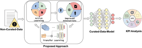
Figure 1 presents the proposed data quality framework. From left to right, we start with non-curated data sourced directly from the industrial processes that originally generate it. Subsequently, the framework incorporates three strategic approaches: active learning, enhanced annotations, and transfer/few-shot learning, all directed towards the enhancement of data quality. On the right, the ultimate outcome is a meticulously curated data model that attains the objectives of optimal data quality and the refinement of decision-support models.

Figure 1. Proposed data quality framework: from non-curated data to curated data model.

2.1. Active learning

Active Learning is a machine learning technique that focuses on selectively choosing the most relevant data for training a model. However, when labeling data for a ML model to learn from, data annotators may face several challenges. In agricultural environments, for instance when identifying pests, annotating can be difficult. Pest identification, and particularly insect identification may pose challenges due to their size, anatomy, and visibility (Costa et al., 2023). In such cases, Active Learning (AL) can alleviate the annotators’ efforts.

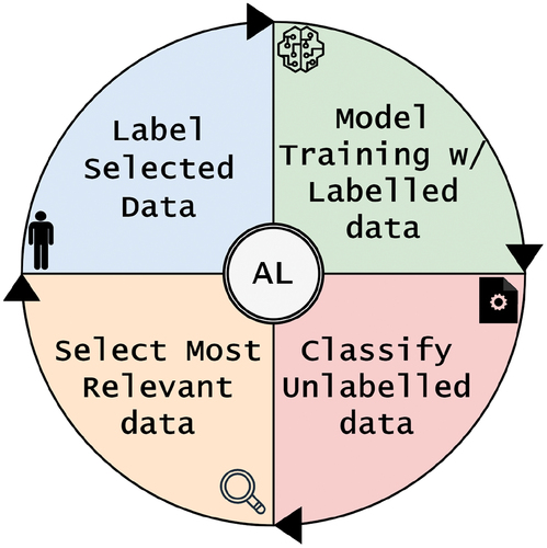
The key to AL is to use a partially trained model to classify unlabeled data. This model’s predictions are employed to rank the data according to levels of uncertainty. Samples with the highest uncertainty are considered the most valuable for further refining the model. These key data points should be labeled by a human expert and then incorporated into the training process. This cycle is repeated until the model reaches a satisfactory level of performance. Figure 2 summarizes the AL cycle, including model training with labeled data, classification of unlabeled data, selection of most relevant data, and label selected data.

Figure 2. Representation of active learning steps: model training with labeled data, classification of unlabeled data, selection of most relevant data, and label selected data.

Active learning can be divided into stream-based or pool-based approach (Hsu & Lin, 2015). In a stream-based method, data is continuously fed to the learning model one at a time from a specific distribution. For each data item, the model must quickly decide whether or not to request its label. In a pool-based method, the model starts with two sets of data: one with unlabeled samples, denoted $D_u=x_1,x_2,\dots ,x_n$, and another with labeled samples, denoted $D_l=(\mathit{x}{{\mathit{ }}^{\mathrm{\prime }}}_1,\mathit{y}{{\mathit{ }}^{\mathrm{\prime }}}_1),(\mathit{x}{{\mathit{ }}^{\mathrm{\prime }}}_2,\mathit{y}{{\mathit{ }}^{\mathrm{\prime }}}_2),\dots ,(\mathit{x}{{\mathit{ }}^{\mathrm{\prime }}}_{\mathit{m}},\mathit{y}{{\mathit{ }}^{\mathrm{\prime }}}_{\mathit{m}})$, where $\mathit{y}{{\mathit{ }}^{\mathrm{\prime }}}_{\mathit{i}}$ is the label for $\mathit{x}{ }^{\mathrm{\prime }}\mathit{i}$. Initially, a learner trains a classifier $f_0$ using $D_l$. Then, in each iteration ($\mathit{t}=1,2,\dots ,\mathit{T}$), the learner, with the previous classifier $\mathit{ft}-1$, selects a data point $x_j$ from $D_u$, asks for its label $y_j$, and adds the labeled pair $(x_j,y_j)$ to $D_l$. This process helps to train a new classifier $f_t$ with the updated $D_l$. The goal is to achieve the highest precision for $f_t$ when using a separate set of $D_l$.

AL can enhance the effectiveness of ML by decreasing the volume of data required for training, leading to a model that performs adequately. This method can reduce the time spent on both labeling and training activities, and it also reduces the workload on experts who might be required to label the data.

2.2. Improved annotations

Numerous studies concentrate on enhancing the architecture of ML models to achieve better performance and minimize the resources and time spent training (Zha et al., 2023). In contrast, Data-Centric AI approaches prioritize improving data quality, including the quality of labels or annotations, over refining the model design.

In agricultural settings, decision support models exert substantial influence, guiding critical decisions such as pharmacological interventions or crop harvesting. When data annotations are unreliable by noise, bias, or inaccuracies, these decisions can lead to erroneous outcomes, posing the risk of severe environmental and financial repercussions.

Many studies have underscored the significance of label quality in ML models. In (Ma et al., 2022), the authors identified incorrect and missing labels in well-known datasets, such as MS COCO and Google Open Images. They meticulously re-annotated these datasets and examined the benefits of their actions. Another study in (Northcutt et al., 2021) emphasized the importance of having a high-quality and real-world representative test set. The comparison of ML model performance is often based on the accuracy achieved on the test set. Consequently, a test set with errors or one that does not accurately represent real-world scenarios can lead to incorrect decisions when selecting the best model for a specific task.

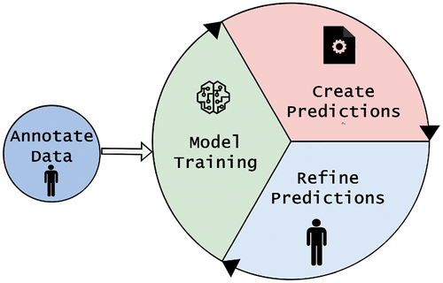
The annotation process can be difficult and time-consuming, which may lead to errors by the annotators (Martin-Morato & Mesaros, 2023). These errors can affect the performance of the models. However, these models can still perform satisfactorily enough to produce labels or annotations, sometimes with greater precision than the erroneous ones created by the annotators. Models with erroneous or missing annotations can still be beneficial, providing predicted annotations for new images as a starting point. Human experts can then use these predictions to correct and annotate any missing or faulty data (Sylolypavan et al., 2023). This process of utilizing model predictions to rectify and enhance annotations allows for the training of new models that outperform their predecessors, demonstrating continuous improvement in model accuracy and reliability. Figure 3 illustrates the process we propose to produce improved annotations.

Figure 3. Diagram of our method’s process for improving annotations.

2.3. Transfer learning

The landscape of Machine Learning has undergone a remarkable evolution, with the emergence of Deep Learning standing out as a transformative force. This paradigm shift has not only revolutionized traditional approaches but has also propelled the field into new complexity levels, enabling the development of sophisticated models capable of extracting intricate patterns and insights from vast and diverse datasets.

In agricultural applications, the possibility of grasping powerful models has propelled agriculture 4.0 and supported different activities and applications, such as, industrialization, security, traceability, and sustainable resource management (Jasim & Fourati, 2023).

Nonetheless, a downfall of Deep learning (DL) is that it requires abundant data to effectively learn, making it less suitable in situations with limited data availability. To address this issue, Few-Shot Learning (FSL) was developed. It enables DL models to learn from a small number of examples. This approach aims to make machine learning more similar to how humans learn, quickly grasping new concepts from just a small amount of information (Parnami & Lee, 2022). These approaches are generally categorized into two types: meta-learning and non-meta-learning algorithms. A meta-learner consistently modifies the model’s parameters, allowing it to adapt to new experimental tasks using a minimal amount of labeled data.

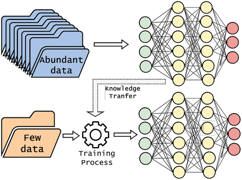
Transfer Learning (TL) falls under the non-meta-learning category. This method utilizes the experience a model has acquired from executing tasks that are similar but not exactly identical. Figure 4 illustrates the TL process.This strategy saves time and resources, enhancing the efficiency of ML.

Figure 4. Overview of transfer learning: a new model is initiated with the weights of a pre-trained model, facilitating its training process.

A domain is represented as $\mathcal{D}=\mathcal{X},\mathit{P}(\mathit{X})$, with $\mathcal{X}$ being the feature space and $\mathit{P}(\mathit{X})$ the marginal probability distribution. A task $\mathcal{T}$ is defined by a label space $\mathit{Y}$ and a predictive function $\mathit{f}(.)$ (Pan & Yang, 2010).

In the scenario of TL, given a source domain ${\mathcal{D}}_s$ and its corresponding task ${\mathcal{T}}_s$, alongside a target domain ${\mathcal{D}}_t$ and target task ${\mathcal{T}}_t$, the goal of TL is to enhance the learning of the target predictive function $f_t(.)$ in ${\mathcal{D}}_t$. This is achieved by leveraging the knowledge from ${\mathcal{D}}_s$ and ${\mathcal{T}}_s$, where ${\mathcal{D}}_s\ne {\mathcal{D}}_t$, or ${\mathcal{T}}_s\ne {\mathcal{T}}_t$. Specifically in object detection model training, TL is often employed by initializing a model with pre-trained weights. This approach ensures that the training does not start from zero, as the model is already equipped with some understanding of a related task

2.4. Key performance indicators

To complement the framework we define six Key Performance Indicators (KPI) depicted in Figure 5 and described as follows:

Figure 5. Key performance indicators for data quality.

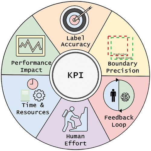
(1) Label Accuracy (LA): Label accuracy measures the correctness of annotations or labels assigned to data points. It quantifies the percentage of accurately labeled instances in comparison to the total labeled data, indicating the precision of the labeling process.

(2) Boundary Precision (BP): Boundary precision evaluates the accuracy and specificity of defining boundaries or edges in annotated data, especially in tasks like image segmentation or object detection. It assesses how precisely annotated boundaries align with the actual edges of objects or features.

(3) Feedback Loop (FL): Feedback loop evaluates the effectiveness of incorporating feedback or corrections into the data annotation process. It measures how efficiently errors or discrepancies identified during annotation are addressed, corrected, and integrated to improve future annotations.

(4) Human Effort (HE): Human effort quantifies the amount of time, labor, or resources expended by annotators or individuals involved in the data labeling process. It assesses the workload and resource investment required to produce high-quality annotations.

(5) Time and Resources (TR): Time and resources measure the efficiency of the data annotation process by evaluating the time and resources utilized to complete the labeling tasks. It assesses whether the process is optimized in terms of time efficiency and resource allocation.

(6) Performance Impact (PI): Performance impact evaluates how data quality influences the performance of machine learning models or downstream applications. It assesses the direct impact of high-quality annotations on the accuracy, robustness, and effectiveness of models trained on labeled data.

The evaluation of the KPI is carried out in three levels:

(1) This top-level rating represents the highpoint of performance, with a score of 1 signifying optimal achievement. It indicates that the method excels, demonstrating the best possible outcomes under the specified KPI.

(2) Positioned as an intermediate level, a score of 2 denotes a commendable performance, though not reaching the possible maximum. It signifies strong effectiveness compared to alternatives, positioning the method as a high-performing solution under the specified KPI.

(3) This bottom-level rating indicates a lower level of performance, with a score of 3 suggesting that the method falls short in comparison. It serves as a reference point for lower effectiveness under the specific KPI.

Our defined set of KPIs encompasses critical metrics specifically designed to assess various aspects of data annotation quality and its impact on downstream processes. These KPIs were carefully selected based on their relevance to the primary objectives of our study and validated through rigorous testing and expert consultation, ensuring their accuracy and reliability in measuring performance improvements and their alignment with industry standards. Label Accuracy (LA) serves as a fundamental measure, quantifying the precision of annotations by evaluating the correctness of labels assigned to data points. Boundary Precision (BP) extends this assessment by scrutinizing the accuracy of delineating object boundaries, crucial for tasks like image segmentation. Meanwhile, Feedback Loop (FL) evaluates the efficacy of integrating feedback into the annotation process, ensuring continual improvement and error correction. Human Effort (HE) and Time and Resources (TR) provide valuable insights into the labor and resource investment required for annotation tasks, guiding efficient resource allocation. Finally, Performance Impact (PI) elucidates the direct correlation between data quality and the performance of machine learning models or downstream applications, emphasizing the pivotal role of high-quality annotations in enhancing model accuracy and effectiveness. Together, these KPIs offer a comprehensive framework for evaluating data annotation quality, ensuring the robustness and efficacy of annotated datasets in driving subsequent analyses and decision-making processes.

This method harnesses established techniques within a novel context. While the methodologies employed are well-documented in literature, their application in the field of data annotation quality for smart farming represents an innovative feature. By adapting and integrating these techniques into our framework, we introduce a fresh perspective that enhances their efficacy and applicability. This strategic amalgamation not only underscores our innovative approach but also showcases the transformative potential of established methodologies when deployed in new and innovative contexts.

3. Materials and results

In this section we describe the farming industry problem that was chosen to demonstrate the framework. We further detail on the data that was used and the evaluation metrics defined. Finally, we also present the results achieved for the framework’s components.

3.1. Problem description

Among the numerous factors that can affect crop yields, pests are a significant contributor to losses. For instance, in tomato greenhouses, the whitefly pest is one of the most common and detrimental pests (Nieuwenhuizen et al., 2018). In (Cardoso et al., 2022), a novel system was proposed, consisting of yellow sticky traps with cameras mounted above, to detect and count this pest within tomato plantations. This system relies not only on the number and location of each trap but also on the high resolution and controlled setting in which the images are captured. Although the system has shown outstanding results, there is room for improvement, as it could be more accurate in detecting whiteflies in their natural habitat, which are the plant leaves.

To create a system that more accurately represents real-world conditions, it is necessary to have images that mimic these scenarios. The source for this system comprises carefully captured images, in order to reduce natural noise due to different light conditions or due to the presence of elements like dust or other insects, and requires meticulous annotation, as annotations in noisy environments demand extra effort from human experts. This process is essential for the creation of a dataset that enables the training of a machine learning model to detect whitefly pest in images or videos within their natural habitat.

3.2. Dataset

In pursuit of images depicting whiteflies in their natural habitat, and recognizing the need for a foundational dataset for machine learning in a field with limited data, initiating a data collection process was essential. Consequently, we captured images in a tomato greenhouse in Coimbra, Portugal. This greenhouse, measuring 100 m$\times$200 m, is organized in rows of tomato plants. To ensure a diverse dataset, encompassing variations in light exposure and plant shapes influenced by their positioning, we selected three different rows for image capture.

Aiming for more realistic scenarios, images were recorded using two different mobile devices, each with unique characteristics and image resolutions. The first device captured 300 images at a resolution of 4000$\times$3000 pixels, while the second recorded 200 images at 3000$\times$4000 pixels. This strategic use of devices with different resolutions and characteristics not only mirrors real-world challenges, such as potential out-of-focus shots and hand movements, but also adds complexity to the task of annotating whiteflies, posing an additional challenge for experts.

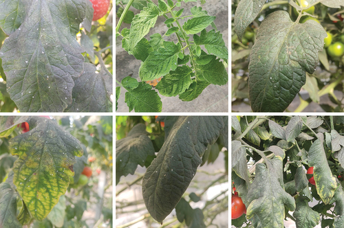
After the images were collected from the tomato greenhouse, each was resized to a resolution of 3000$\times$3000 pixels to ensure consistency across the dataset. Figure 6 displays a collection of six images recorded during this process, exemplifying its diversity due to different conditions in the greenhouse environment.

Figure 6. Collection of images captured in a tomato greenhouse in Coimbra, Portugal, showcasing the diverse environmental conditions within the greenhouse. These images highlight different row arrangements and light exposures.

The captured images feature tomato plants against varied backgrounds and under different lighting conditions, all infested with whitefly pests. These pests are quite diminutive, measuring 1 to 3 mm in length (Sani et al., 2020) and each image might include as many as 70 flies.

Out of the 500 images captured, a subset of 200 was randomly selected for annotation to alleviate the complexities of the task. These images were chosen from the device that captured images at a resolution of $4000\times 3000$. The annotation process employed the labelImg tool, enabling the use of a computer mouse to draw bounding boxes around each whitefly, subsequently labeled as ‘whitefly’. Considering the aforementioned challenges, including the high density of whiteflies per image and the varied image scenarios, the annotation task proved to be highly repetitive and thus susceptible to errors. During annotation, no stringent guidelines were applied, and all white marks in the images were considered potential targets for detection.

Among the 200 images 10,747 whiteflies were identified and marked, averaging approximately 54 whiteflies in each image. The emphasis during the annotation process was on efficiency rather than detailed accuracy, considering the time and resources dedicated to this task.

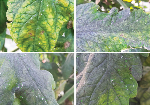
Figure 7 displays four images that have been annotated using the labelImg tool.

Figure 7. Series of images featuring whiteflies annotated using the labelImg tool, illustrating the results of the annotation process.

3.3. Evaluation metrics

To evaluate models designed to detect and count whiteflies in their natural habitat, we employ two different metrics: mean Average Precision (mAP) combined with the training time of the model. The mAP metric is widely used in evaluating object detection models, as it assesses both the accuracy of the predictions and the precision of each prediction’s location. Understanding this metric is crucial, and it involves comprehending the Intersection over Union (IoU), which measures the overlap between the bounding box predicted by the model and the bounding box created by the annotator, also known as the ground truth, as it is assumed to be the correct location of the object to be detected. Figure 8 illustrates IoU calculation, where the green and red dashed squares represent, respectively, the ground truth and the prediction given by the model.

Figure 8. Intersection over Union (Iou) calculation.

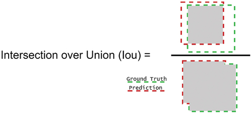
In mAP, an object is classified as a true positive (TP) if IoU$>=0.5$, and as a false positive (FP) otherwise. This classification is based on setting the IoU threshold at 0.5. Average Precision (AP) is determined by calculating the area under the curve (AUC) of the precision-recall curve. This curve plots the model’s precision at varying levels of recall for different confidence thresholds assigned to a bounding box by the model. These thresholds reflect the model’s confidence that a particular bounding box contains an object. The mAP is then calculated by averaging the AP across all classes.

Regarding the training time as a metric, we seek a balance between the mAP performance and the time required to achieve it. A model that achieves similar mAP values but takes less time to train is considered a better model, as it is faster and therefore more efficient.

3.4. Experimental results

To assess the quality of the annotation process under various methods, we conducted three different experiments: one using AL, which focuses on selecting the most relevant images for annotation; another involving automatic enhancement of the annotations; and a third utilizing TL.

3.4.1. Active learning

We conducted an experiment that initially involved training a model with a limited dataset. We then incrementally added more relevant data, as determined by AL techniques, until all the images were utilized.

We randomly divided the 200 images into 160 for training and validation, and 40 for testing. We began the training with 20 images and subsequently used the trained model to classify the remaining 140 images. Following classification, we employed the Bounding Box with a confidence score function to rank the data from most to least relevant. The most relevant images were identified as those with the lowest average confidence in their predictions.

Table 1 summarizes the results of the experiment. Models trained with a limited number of examples fail to yield satisfactory results. Notably, good outcomes are only achieved when the training process involves at least 110 images. An interesting observation is that the model reached optimal performance with 140 images, and further additions did not enhance its performance. This indicates that not all images are necessary to attain peak performance, allowing for a reduction in annotation efforts. Consequently, it can be affirmed that AL techniques can effectively alleviate the annotation process.

Table 1. Results table for the AL experiment presenting the evolution of mean Average Precision (mAP) as a percentage and training time (in seconds) across an incrementally increasing number of images used in the training process, utilizing an NVIDIA GeForce RTX 4080.

# Train. & Val.	mAP (%)		Training time (s)
Images	AL	Random	AL	Random
20	5.9	5.9	289.2	310.2
35	49.5	51.5	386.4	375.5
50	60.4	59.4	463.3	462.9
65	79.4	76.5	472.2	461.1
80	85.8	85.5	548.2	534.5
95	86.6	86.1	612.6	602.4
110	89.5	87.6	672.9	658.9
120	89.4	87	731.6	731.5
130	90.7	90.1	764.9	769.2
140	92.6	91.7	835.3	828.8
150	92	91	890.2	890.7
160	92.6	92.9	932.1	936.5

3.4.2. Improved annotations

During the evolution of the annotation process and preliminary experiments, it was noted that the task was particularly error prone, necessitating high concentration and specific skills due to factors like the size, location, and visibility of whiteflies in the images. Despite these challenges, which resulted in some whiteflies being missed, others incorrectly annotated, and inaccuracies in the bounding boxes, models trained with these datasets not only managed to achieve noteworthy mAP, but sometimes even generated predictions with higher boundary precision than those produced by human experts. Figure 9 provides a visual comparison between an image annotated by a human and one with the predictions of a machine learning model trained using the dataset containing these errors.

Figure 9. Visual comparison highlighting key differences in annotation boundary precision: focusing on the discrepancies in the center points and area sizes of bounding boxes between a poorly annotated image and a properly annotated one.

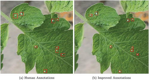
It was observed that the predictions made by the ML model sometimes surpassed the quality of our annotations, particularly in terms of the accuracy of the center points and the sizes of the bounding boxes. To scientifically validate this observation, we conducted an experiment comparing ML models trained on two different datasets: one with our erroneous annotations and the other with predictions made by an ML model.

For a fair comparison, both models were tested against the same test set. To this end, we randomly selected 40 images. Using the predictions from the preliminary experiments as a base, we initiated a re-annotation process for these selected images. This process was guided by specific guidelines that clearly defined what should and should not be annotated as whiteflies. The criteria included identifying ‘V’ shapes, triangular shapes, or focused sharp white forms as whiteflies.

Following this process, we ended up with two datasets and one test set. The two datasets contained the same 160 images but differed in annotations: one set had annotations made by humans and the other by a machine. The test set comprised 40 images annotated by a machine but refined by a human.

For the training process, we split the dataset into 60% for training and 20% for validation, and trained two models using the same images but with different annotations. Since the division of the training and validation sets was done randomly, we conducted the experiment 30 times to ensure robustness and reliability in our findings. The results of these repeated trials are presented in Table 2.

Table 2. Results obtained on the improved annotations experiment: the average mean Average Precision (mAP) and the training time (Train. Time) are presented with standard deviation in parentheses over 30 runs, utilizing an NVIDIA GeForce RTX 4080.

Annotations	mAP (%)	Train. Time (s)
Human	90.44 (0.70)	758.20 (5.76)
Machine	91.54 (0.66)	760.69 (3.62)

The results obtained from the experiment demonstrate that enhancing annotations with the assistance of a machine leads to an advantage in mAP performance. On average, there was an improvement of 1.1 mAP points when using machine-enhanced annotations. However, this improvement comes at the cost of increased computational time, as training with the Improved Annotations was, on average, 2.49 seconds slower.

Since no extra effort was required to produce better quality annotations, it is reasonable to affirm that machine-enhanced annotations can indeed benefit the annotation process. This approach not only alleviates human effort but also has the potential to save time and streamline the overall process.

3.4.3. Transfer learning

We conducted an experiment using TL from a model that was previously trained to detect whiteflies in a completely different scenario from ours. This model had been trained on high-resolution images of yellow sticky traps under regulated light exposure, with minimal environmental variations (Cardoso et al., 2022). Our objective was to determine whether it was possible to train a model with less data and still achieve satisfactory results by employing TL. Using less data translates to reduced annotation efforts and increased efficiency in ML training.

The experiment involved training two models using the same image set, but we approached the training across different scenarios. Initially starting with no training images, we incrementally added images to the dataset. The models differed in their methods of weight initialization: one used the weights from the pre-trained model for detecting whiteflies on yellow sticky traps, while the other had weights initialized randomly. Table 3 summarizes the results, presenting the average mAP and training times of the models across 5 trials.

Table 3. Comparison of models trained with the same image set but different weight initialization methods: ‘TL’ (Transfer Learning with pre-trained model weights) and ‘Random’ (randomly initialized weights). The number of images used in the training process (# Images), mAP results, and training times (Train. Time) are outlined for each approach. The models were trained using an NVIDIA GeForce RTX 4080.

# Images			mAP (%)		Train. Time (s)
Total	Train.	Val.	TL	Random	TL	Random
0	-	-	2	0	-	-
2	1	1	16	0	255	248
4	2	2	18	0	210	241
7	5	2	19	0	227	253
15	10	5	35	0	245	287
20	15	5	42	4	298	346
30	20	10	56	23	300	373
50	40	10	62	34	405	443
160	120	40	77	68	917	962

The results demonstrated a significant advantage in employing TL for training a model. Compared to random weight initialization, TL consistently outperformed in both mAP and training time, averaging improvements of 24% and 10%, respectively.

Although acceptable results were only achieved in the final setup using 160 images, it is possible to affirm that TL can alleviate annotation efforts. This is evidenced by the fact that the random initialization method did not achieve the same performance with an equivalent number of images. This implies that more images would likely be required for training with random initialization, thereby increasing the annotation efforts.

3.4.4. Our approach

In an effort to further explore the impact of our findings, we conducted an experiment that simultaneously addressed three approaches: training a model using TL, AL, and improved annotations, a strategy we refer to as ‘Our Approach’.

The process began by randomly selecting 16 images alongside their improved annotations for training an initial model using transfer learning from the model trained in (Cardoso et al., 2022). This model was then used to rank the remaining images, and the 16 next images with least confidence average on the prediction were select for the subsequent training iteration. This process was repeated until all the 160 images were selected.

For comparative analysis, we trained another model using the same initial set of images as Our Approach, which we denote as ‘Baseline’. Unlike Our Approach, the Baseline model started its training with randomly initialized weights and employed annotations considered to be of inferior quality. Moreover, the Baseline model diverged further by adding supplementary sets of images in each iteration through random selection.

In each iteration, the sets of 16 images selected were randomly divided into 75% for training and 25% for validation. To account for the random selection factor, we replicated the experiment 30 times. The average results concerning mAP achieved on the test set and training time across these 30 runs are detailed in Table 4.

Table 4. Comparison of our approach utilizing Active Learning (AL), Transfer Learning (TL), and improved annotations versus the Baseline method with no AL, no TL, and human-produced annotations. The key metrics presented include the number of images used in training (# Images), and the averages of mean Average Precision (mAP) results, and training durations (Train. Time) over 30 runs. All models underwent training on an NVIDIA GeForce RTX 4080. Note: The setup in which the Baseline model achieved its best performance is highlighted in red, while the setup in which Our Approach initially surpassed the configuration highlighted in red, as indicated by the green marker.

# Images			Train. Time (s)		mAP (%)
Total	Train.	Val.	Our Approach	Baseline	Our Approach	Baseline
16	12	4	341	400	0.806	0.163
32	24	8	351	434	0.904	0.632
48	36	12	453	520	0.918	0.774
64	48	16	479	634	0.92	0.795
80	60	20	626	714	0.923	0.875
96	72	24	602	796	0.924	0.886
112	84	28	823	910	0.926	0.904
128	96	32	764	1016	0.926	0.91
144	108	36	895	1107	0.931	0.913
160	120	40	961	1189	0.934	0.917

Our Approach, as expected, consistently outperformed the Baseline, especially in the initial setups. This trend can be clearly observed in Figure 10, where the Baseline curve gradually approaches that of Our Approach in each iteration, however, it never surpasses it.

Figure 10. Comparison of mAP achievements: our approach vs. Baseline. The chart displays the progression of mAP for each approach across various setups. The red dot represents the best performance achieved by the baseline while the green dot indicates the initial setup where our approach outperforms the best of the baseline.

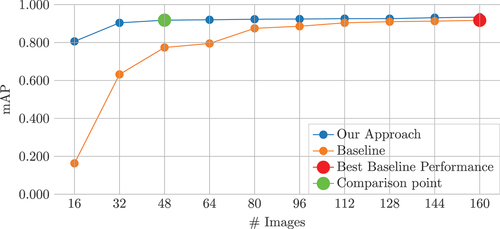
The Baseline reached its peak performance, achieving a 91.7% mAP with 160 images. In contrast, Our Approach surpassed it by 0.1 mAP points with only 48 images, representing a reduction of 70% in data usage (112 images).

In terms of training time, the Baseline model, on average, took 1189 seconds to train with 160 images. In contrast, Our Approach completed training with 48 images in just 453 seconds, making it 62% faster. However, it is important to note that Our Approach utilized AL, necessitating antecedent training iterations. Therefore, to attain its performance, the times from the two preceding iterations, 341 and 352 seconds, must be considered, totaling 1145 seconds. This duration is still faster than the Baseline, showcasing the efficiency of Our Approach.

Comparing training times becomes irrelevant when an additional 112 images are needed to achieve similar performance. In contrast, the time and human effort required to annotate such a quantity of images are undoubtedly relevant. Although annotation times were not recorded, we estimate an average of 10 minutes per image, equating to 18.6 hours of human effort.

These achievements highlight the significant impact our approach can have on data curation. By integrating the three techniques, we can substantially reduce both human effort and machine time in developing superior models.

4. Discussion of results

The experiments conducted provided insights into how active learning, enhanced annotations, and transfer learning can influence the efforts required for annotations. Table 5 presents the analysis of the Key Performance Indicators defined in Section 2.3 for the components of the data quality framework. Each component of the framework was ranked from 1 to 3 for the respective KPI as also described in Section 2.3. When an approach has a rank of 1 for a specific Key Performance Indicator it implies superior performance in that particular context.

Table 5. KPI analysis for the different data quality framework components. KPI: Label Accuracy (LA), Boundary Precision (BP), Feedback Loop (FL), Human Effort (HE), Time and Resources (TR), and Performance Impact (PI). Lower ranks represent better KPI evaluation.

KPI	Active Learning	Improved Annotations	Transfer Learning
Label Accuracy	1	3	2
Boundary Precision	3	1	2
Feedback Loop	3	2	1
Human Effort	3	2	1
Time and Resources	1	3	2
Performance Impact	3	2	1
Average	2.33	2.16	1.50

4.1. Label accuracy

Label Accuracy for this experimental setup specifically measures how accurately whiteflies are effectively labeled as whiteflies. For Active Learning, where the most relevant images are selected for being annotated by an expert, it is assumed that the expert correctly labels the whiteflies and does not misidentify it as another class. Consequently, this approach is ranked 1 in terms of Label Accuracy.

In the case of Transfer Learning, the model was not only trained with a specific dataset but also possesses prior knowledge about the task. This suggests that it is less likely to incorrectly classify labels compared to the Improved Annotations approach. Therefore, the latter is ranked 3 and the first is ranked 2 for Label Accuracy.

4.2. Boundary precision

Boundary Precision is associated with the precision of the bounding boxes around objects, whiteflies in this scenario. The experiments demonstrated that ML models may predict the location of whiteflies with higher precision compared to human annotations. As a result, the Improved Annotations approach, which benefits from the precision of ML models, is ranked as 1 in terms of Boundary Precision.

On the other hand, the Active Learning approach requires annotations by an expert. Since human annotation is prone to errors and potential imprecision in the bounding boxes, it is ranked as 3 in Boundary Precision. This ranking reflects the comparative advantage of machine-aided annotations in achieving more accurate boundary delineation.

4.3. Feedback loop

Feedback loop is originated by the common fact that in ML the output of the system is somehow systematically fed back into the system as a way of promoting the learning process. While this usually has a desirable effect, it can promote or exacerbate existing biases within a system from different sources, e.g. data, algorithms, feedback amplification, etc.

Transfer Learning is the approach that exhibits less errors, this it is the highest ranked. Active Learning is ranked 3 since the choice of active examples may not be protected against data and algorithm bias. Improved Annotations is ranked 2, since it does not suffer from the Active Learning disadvantages neither from the Transfer Learning advantages.

4.4. Human effort

For Human Effort, Active Learning necessitates human experts to annotate the selected data. When compared to the Improved Annotations technique or Transfer Learning, it is undoubtedly the most demanding in terms of human effort, and thus it is ranked as 3.

In the comparison between Improved Annotations and Transfer Learning, the former utilizes machines to enhance human annotations. However, these machine-enhanced annotations might still require human verification, as was the case in our test set for the respective experiment. Consequently, we rank the Improved Annotations approach as 2 in terms of Human Effort.

Transfer Learning, on the other hand, is ranked as 1 because it has a significant advantage in reducing the number of images needed for training. Fewer images imply less annotation effort, a conclusion supported by our experiment. Its efficiency in utilizing pre-existing knowledge from other models translates into less human input for training, making it the most efficient approach in terms of minimizing human effort.

4.5. Time and resources

For Time and Resources, Active Learning aims to reduce the number of samples used in the training process, which implies less time and resources being utilized. Consequently, it is ranked as 1 due to its efficiency in these aspects.

Both the Improved Annotations and Transfer Learning techniques require a pre-trained model. Improved Annotations use this pre-trained model to generate predictions that serve as annotations, while Transfer Learning uses the pre-trained model as a foundational knowledge base for the new model to learn from. In our experiments, it was observed that its use can reduce training time by about 10 pp., which signifies some savings in computational time. Thus, it is ranked as 2 after Active Learning in this respect.

On the other hand, the Improved Annotations approach, while benefiting from machine predictions, does not inherently reduce computational time as significantly as the others. Therefore, Improved Annotations is ranked as 3 for Time and Resources. This ranking reflects the relative efficiency of each approach in terms of the time and resources required for the model training process.

4.6. Performance impact

In relation to the impact on performance when using each approach versus not using it, Transfer Learning emerges as the most advantageous. It significantly reduces training time and improves mAP performance. Therefore, in this context, it is ranked as 1.

Conversely, Active Learning shows the least impact. When compared to a random selection approach, the improvements with AL were not as pronounced, leading to its ranking as 3 in terms of performance impact.

Meanwhile, the Improved Annotations approach, which enhances human annotations with machine predictions, has a moderate impact. It improves upon basic human annotations but does not achieve the same level of efficiency and performance boost as Transfer Learning. Consequently, Improved Annotations is ranked as 2, reflecting its intermediate status in terms of enhancing performance.

Finally, averaging the results obtained, Transfer Learning is the best performing technique to achieve better data quality in our smart farming scenario. Noteworthy, it is the technique that requires less human effort, and this is particularly relevant when highly qualified annotators are required in the annotation process, as it is the case.

5. Conclusions and future work

In this work, a comprehensive framework was introduced to tackle challenges related to data annotation quality in the context of smart farming. The presented case study included a whitefly pest detection problem in images. To address this issue three methods were proposed, namely active learning, transfer learning, and automatic annotation enhancement.

For further evaluation a set of six Key Performance Indicators (KPI) were defined and the experimental results allowed us to conclude how the proposed techniques can influence the efforts required for annotations.

The findings of this work underscore the importance of leveraging advanced techniques such as transfer learning in addressing data annotation challenges within smart farming contexts. With transfer learning demonstrating superior annotation quality in our case study, particularly in scenarios where highly skilled annotators are scarce, its adoption holds significant promise for enhancing annotation efficiency and accuracy. This highlights the critical role of methodological innovation in optimizing data annotation processes and ultimately improving decision support systems in smart farming.

As we look ahead, this framework lays the groundwork for several promising avenues of future research. Firstly, there is an opportunity to extend the applicability of the framework to diverse learning scenarios, including multiclass classification and regression problems, thereby broadening its utility across various agricultural domains. Additionally, integrating multimodal data, such as tabular, audio, and text data, offers a compelling direction for enhancing the framework’s versatility and applicability in different production and manufacturing contexts. Further research could also explore the framework’s adaptation to real-time data processing environments, enabling more dynamic and responsive decision support systems. By pursuing these future directions, we can enhance the effectiveness and adaptability of our framework, advancing the state-of-the-art in data annotation methodologies for smart farming and beyond.

Acknowledgments

This work was supported by project PEGADA 4.0 (PRR-C05-i03-000099), financed by the PPR - Plano de Recuperação e Resiliência and by national funds through FCT, within the scope of the project CISUC (UID/CEC/00326/2020).

Disclosure statement

No potential conflict of interest was reported by the author(s).

Data availability statement

The data will be made available upon acceptance of the paper.

Additional information

Funding

The work was supported by the Fundação para a Ciência e a Tecnologia [PRR-C05-i03-000099].

References

- Cardoso, B., Silva, C., Costa, J., & Ribeiro, B. (2022). Internet of things meets computer vision to make an intelligent pest monitoring network. Applied Sciences, 12(18), 9397. https://doi.org/10.3390/app12189397
- Cardoso, B., Silva, C., Costa, J., & Ribeiro, B. (2023). Edge computing with low-cost cameras for object detection in smart farming. In S. Lopes, P. Fraga-Lamas, & T. Ferna´ndes-Cam´ares (Eds.), Smart technologies for sustainable and resilient ecosystems (pp. 16–22). Springer Nature Switzerland.
- Chen, Y., Santosa, A. E., Yi, A. M., Sharma, A., Sharma, A., & Lo, D. A. (2020). A machine learning approach for vulnerability curation. 2020 IEEE/ACM 17th International Conference on Mining Software Repositories (MSR) (pp. 32–42.
- Costa, D., Silva, C., Costa, J., & Ribeiro, B. (2023). Enhancing pest detection models through improved anno- tations. In N. Moniz, Z. Vale, & J. Cascalho (Eds.), Progress in artificial intelligence (pp. 364–375). Springer Nature Switzerland.
- Hsu, W. N., & Lin, H. T. (2015, February). Active learning by learning. Proceedings of the AAAI Conference on Artificial Intelligence, 29(1). https://ojs.aaai.org/index.php/AAAI/article/view/9597
- Jasim, A. N., & Fourati, L. C. (2023). Agriculture 4.0 from iot, artificial intelligence, drone, & blockchain perspectives. 2023 15th International Conference on Developments in eSystems Engineering (DeSE), Baghdad & Anbar, Iraq. (pp. 262–267).
- Kusy, B., Liu, J., Saha, A., Li, Y., Marchant, R., Oorloff, J., & Oerlemans, A. (2022, October). In-situ data curation: A key to actionable ai at the edge. MobiCom ‘22: Proceedings of the 28th Annual International Conference on Mobile Computing And Networking, Sydney NSW Australia. (pp. 794–796).
- Lafia, S., Thomer, A., Bleckley, D., Akmon, D., & Hemphill, L. (2021). Leveraging machine learning to detect data curation activities. 2021 IEEE 17th International Conference on eScience (eScience), Innsbruck, Austria. (pp. 149–158).
- Ma, J., Ushiku, Y., & Sagara, M. (2022). The effect of improving annotation quality on object detection datasets: A preliminary study. 2022 IEEE/CVF Conference on Computer Vision and Pattern Recognition Workshops (CVPRW), New Orleans, LA, USA. (pp. 4849–4858).
- Martin-Morato, I., & Mesaros, A. (2023). Strong labeling of sound events using crowdsourced weak labels and annotator competence estimation. IEEE/ACM Transactions on Audio, Speech, and Language Processing, 31, 902–914. https://doi.org/10.1109/TASLP.2022.3233468
- Nieuwenhuizen, A. T., Hemming, J., & Suh, H. K. (2018). Detection and classification of insects on stick- traps in a tomato crop using faster r-cnn. The Netherlands Conference on Computer Vision. https://api.semanticscholar.org/CorpusID:69451220
- Northcutt, C. G., Athalye, A., & Mueller, J. (2021). Pervasive label errors in test sets destabilize machine learning benchmarks. arXiv preprint arXiv:210314749.
- Pan, S. J., & Yang, Q. (2010). A survey on transfer learning. IEEE Transactions on Knowledge and Data Engineering, 22(10), 1345–1359. https://doi.org/10.1109/TKDE.2009.191
- Parnami, A., & Lee, M. (2022). Learning from few examples: A summary of approaches to few-shot learning. arXiv preprint arXiv:220304291.
- Rangineni, S. (2023). An analysis of data quality requirements for machine learning development pipelines frameworks. International Journal of Computer Trends and Technology, 71(8), 16–27. https://doi.org/10.14445/22312803/IJCTT-V71I8P103
- Rosero, R., Silva, C., Ribeiro, B., & Santos, B. F. (2023). Label synchronization for hybrid federated learn- ing in manufacturing and predictive maintenance. Journal of Intelligent Manufacturing, 1–20. Springer. https://doi.org/10.1007/s10845-023-02298-8
- Sani, I., Ismail, S. I., Abdullah, S., Jalinas, J., Jamian, S., & Saad, N. (2020). A review of the biology and control of whitefly, Bemisia tabaci (Hemiptera: Aleyrodidae), with special reference to biological control using entomopathogenic fungi. Insects, 11(9), 619. https://www.mdpi.com/2075-4450/11/9/619
- Subramaniyan, M., Skoogh, A., Salomonsson, H., Bangalore, P., Gopalakrishnan, M., & Sheikh Muhammad, A. (2018). Data-driven algorithm for throughput bottleneck analysis of production systems. Production and Manufacturing Research, 6(1), 225–246. https://doi.org/10.1080/21693277.2018.1496491
- Sylolypavan, A., Sleeman, D., Wu, H., & Sim, M. (2023). The impact of inconsistent human annotations on ai driven clinical decision making. IEEE/ACM Transactions on Audio, Speech, and Language Processing, 6(1), 26. https://doi.org/10.1038/s41746-023-00773-3
- Tran, N., Chen, H., Bhuyan, J., & Ding, J. (2022). Data curation and quality evaluation for machine learning-based cyber intrusion detection. Institute of Electrical and Electronics Engineers Access, 10, 121900–121923. https://doi.org/10.1109/ACCESS.2022.3211313
- Wuest, T., Weimer, D., Irgens, C., & Thoben, K.-D. (2016). Machine learning in manufacturing: advantages, challenges, and applications. Production and Manufacturing Research, 4(1), 23–45. https://doi.org/10.1080/21693277.2016.1192517
- Zangeneh, M., Akram, A., Nielsen, P., & Keyhani, A. (2015). Developing location indicators for agricultural service center: a delphi–topsis–fahp approach. Production and Manufacturing Research, 3(1), 124–148. https://doi.org/10.1080/21693277.2015.1013582
- Zha, D., Bhat, Z. P., Lai, K. H., Yang, F., Jiang, Z., Zhong, S., & Hu, X. (2023). Data-centric artificial intelligence: A survey. arXiv preprint arXiv:230310158.