Deep learning-supported machine vision-based hybrid system combining inhomogeneous 2D and 3D data for the identification of surface defects

ABSTRACT

Machine vision systems for automatic defect detection commonly adopt 2D image-based systems or 3D laser triangulation systems. 2D and 3D systems present opposite advantages and disadvantages depending on the typology and position of defects to be detected. When the variety of defects is large, none of them performs defect detection accurately. To overcome this limitation, this paper illustrates a hybrid Deep Learning-supported system where the 2D- and 3D-generated data are juxtaposed and analyzed contextually. Anomaly scores are subsequently determined to distinguish suitable and uncompliant parts. The implementation of the hybrid system allowed the identification of defective parts in an aluminium die-cast component with an accuracy concerning true positives of over 95% by comparing the system outputs with human defect detection. The inspection time was reduced by approximately 20% if compared, once again, with the same activities performed by humans.

KEYWORDS:

• Surface defects analysis
• hybrid 2D and 3D system
• machine vision systems
• deep learning
• high-pressure die-casting

1. Introduction

The current requirements of the manufacturing industry include the achievement of ever better product quality performances, which is largely supported by applications based on Artificial Intelligence (Ördek et al., 2024). The need for quality control during manufacturing or immediately after the production is increasingly emphasized (Kim et al., 2018; Savio et al., 2016; T. Wang et al., 2018). Specific attention is on surface imperfections that exceed acceptable levels, i.e. surface defects appearing on manufactured surfaces (Mullany et al., 2022), such as scratches, cold joints, and stains. Such defects negatively affect not only the aesthetics of the product and the comfort of use, but also its performance (Bulnes et al., 2016; Song & Yan, 2013) and safety. The identification of surface defects can take place in the forms of automatic and human visual inspection (Mullany et al., 2022).

Surface defect detection of aluminium castings used in the automotive industry is still performed in a large fraction by means of human vision inspection (Bharambe et al., 2023), in line with other domains (Wu et al., 2018; Xu & Huang, 2021). This applies to the industrial case study presented in this paper too. As a result, specialised operators have developed visual and manual skills to detect most surface defects. Understandably, this task is repetitive and tiring (Xu & Huang, 2021), and a decrease in concentration leads to undesirable variations in the reliability of defect detection, as humans cannot perform with consistent outcomes over extended periods of time (Mullany et al., 2022).

To overcome this issue, research attention has been directed towards Machine Vision Systems (MVS). A recent study (Ren et al., 2022) analyses the current state of the art of defect detection supported by MVS and highlights the increasingly important role of Deep Learning (DL), as well as the difficulties to detect defects in-line for complex parts.

With specific reference to quality inspection, MVS are typically fed by images acquired by a camera or 3D point clouds resulting from a coordinate measuring system, e.g. laser triangulation scanners. More details are provided in the following section, explaining the background of this research. In brief, the use of systems based on 2D imaging, which exhibits outstanding resolutions and efficiency, is limited in terms of identifiable defects (Ye et al., 2019). Coordinate measuring systems can capture the 3D geometry of complex parts (Schöch et al., 2015) including defects having a 3D morphology. However, the massive acquired data relentlessly represents a burden for DL algorithms, inherently leading to limited processing speed (J. Wang et al., 2019). As a consequence, processing times hardly match the required pace of industrial applications. In addition, 3D systems suffer from the complexity of optical imaging, which leads to their scarce diffusion and limited development of systems integrating 2D and 3D information to identify and classify defects (Tang et al., 2023). The starting point of this work is the fact that hybrid 2D/3D systems are poorly diffused according to the literature, while a combination could be deemed beneficial in light of their opposed advantages and disadvantages, as better explained in the following section.

Consistently, the major contribution of this work is the development of an integrated MVS that combines benefits of 2D and 3D optical measuring systems in a common processing pipeline. The main target of such a system is its capability of detecting defects irrespective of their morphology and position, as illustrated in the third section. In addition, the following characteristics, objectives and targets are set for the MVS to be both original in a research perspective and suitable for industrial applications.

1. The capability to combine 2D and 3D sources in a single DL architecture for a batch of parts in the event of needing both data because of the specific shape of the object, defects morphology, and location thereof.

2. Accuracy in the range of both visual inspection (see typical performances of human-based tasks in Section 3) and systems described in the literature for defect detection usable for die-cast aluminium components (see the following section); based on these criteria, the target for this system was set at 90%.

3. Sufficient speed to surpass human visual inspection and to make the system a candidate to replace (at least partially) repetitive human operations.

The next section provides background information on the industrial use of both 2D and 3D MVS along with an overview of the algorithms that allow for their effective implementation. The third section presents the case study chosen as a reference for the development of the hybrid system. The methodology is illustrated in the fourth section, which is earmarked to providing details on the pipeline of data processed through DL in the developed hybrid system. Results are reported in the fifth section, which includes discussions. Conclusions are drawn in the final section.

2. Background and expected performances of a new system

2.1. Use of 2D and 3D data in machine vision systems

A typical industrial 2D-based visual inspection system consists mainly of three modules: optical illumination, image acquisition, image processing and defect detection (DiLeo et al., 2017; Malamas et al., 2003). A previous contribution (Cavaliere et al., 2021) analysed and tested the properties of a 2D MVS system to detect surface defects in aluminium automotive components. This work showed the potential for industrial applications (Silva et al., 2018). MVS significantly improves the efficiency, quality and reliability of defect detection. In MVS-supported inspection, optical illumination platforms and adequate hardware for image acquisition are prerequisites for high-quality images. However, the 2D MVS suffer from a number of limitations. As the image of the target object is generated by the light reflected from it, variations in illumination in the field of view can have a negative impact on accuracy. These variations can be originated, for instance, by changes in environmental conditions or artificial lighting. More in details, substantial variations in light intensity in the working environment can adversely affect the sharpness of edges and features appearing in the 2D plane. Furthermore, as 2D MVS are largely affected by these sharp contrasts (and thus the clarity of edges and features) of the object surface, it is difficult to handle very dark or very shiny objects. Despite the existence of various techniques to illuminate an object, they are not yet sufficiently performing for recognizing its edges and features under certain conditions (L. Liu et al., 2020). Eventually, by intrinsic properties of the imaging process, 2D MVS cannot handle the complexity of three-dimensional shapes. This takes place especially in the case of complex parts and assemblies, when dimensions outside the X-Y plane need to be measured.

3D MVS are a possible solution to the above limitations. 3D MVS exploit the possibility of providing depth information through three-dimensional point clouds of precise coordinates. Moreover, 3D MVS are poorly affected by environmental factors, as illumination or contrast are not a problem, especially when detecting defects on geometrically complex surfaces (Sharifzadeh et al., 2018; Tan & Triggs, 2007). As suggested in the introducing section, drawbacks of 3D MVS are mainly related to acquisition or processing times (as they are typically slower than their 2D counterparts), which discourage their use when alternative systems are sufficiently performing.

2.2. Deep learning approaches for 2D and 3D machine vision systems

As mentioned, the application of DL plays an increasingly important role in the development of the MVS field (Ren et al., 2022). The emergence of DL has given rise to radical changes to the research in this field as it improves the accuracy of image recognition to a level close to or even higher than that of humans (S. Qi et al., 2020). The key modelling framework promoting the achievement of this goal is the convolutional neural network (CNN) (Gu et al., 2018), which is one of the most successful models of DL technologies currently applied in the industry. An interesting example of the application of this framework is the work of Mery (2020), in which a CNN for detecting defects in castings using X-ray images is presented. In a recent study (Nikolić et al., 2023), porosity defects in aluminium alloys were detected using CNN. The aim of this study was to build a CNN model that can accurately predict porosity defects in light optical microscopy images. To train the model, images of polished samples of different secondary aluminium alloys used in high pressure die casting (HPDC) with a significant number of defects were used. Rahimi et al. (2021) propose an improved, accurate and fast object detection method for industrial inspection and quality control. The proposed method is capable of detecting objects in a manufacturing plant, where speed and accuracy are crucial. The underlying architecture utilises the CNN Darknet-53 network integrated in ‘You Only Look Once’ method in version 3 (YOLOv3). Recently, Duan et al. (2020) highlighted the potential for checking even the smallest casting defects by analysing industrial radiographs of steel castings. This study showed that the mean Average Precision (mAP) of YOLOv3_134 is 26.1% higher than that of the original YOLOv3. The improved network model was able to detect casting defects more quickly and accurately than the original one. Subsequently, this method was applied in industrial production. Parlak and Emel (2023) instead focused on aluminium components made in HPDC and compared the defects found in X-ray images by 12 DL-based object detection methods, and among all, YOLOv5 provided the highest detection accuracy with a mAP of 0.956 (Yue et al., 2007).

As discussed in (Zheng et al., 2021), another set of DL algorithms suitable for the inspection of surface defects is constituted by the unsupervised or semi-supervised learning methods, which were focused on in (Cavaliere et al., 2021, 2022). Most representative methods for defect detection include the auto-encoder (AE) and the generative adversarial network (GAN). AE is a typical unsupervised learning algorithm based on two neural networks called encoders and decoders. It was introduced by Rumelhart et al. (1986) and extended to deep self-coding by Hinton and Salakhutdinov (2006). In order to achieve greater robustness than deep auto-coding, the denoising autoencoder (DAE) (Vincent et al., 2008) adopts an approach that combines corruption and denoising to make learned representations robust to partial corruption of the input model. DAE is one of the most common options for surface defect detection with unsupervised DL algorithms. GAN is an unsupervised learning system introduced by Goodfellow et al. (2014) and subsequently developed further (Schlegl et al., 2019).

In general, AEs are not as efficient as GAN in reconstructing an image. As the complexity of images increases, AEs underperforms GANs since images get blurry, but they are nevertheless highly efficient in certain tasks such as anomaly detection (Jia & Liu, 2023).

In the DAE concept, the input is corrupted by noise, such as random Gaussian noise, and the target is the original noise-free sample. The result is a trained system that does not only reduce dimensionality or find a sparse representation, but also performs denoising. It can be argued that this is an additional regularisation similar to dropout, but essentially applied to the input layers (X. Liu et al., 2019).

2.3. Challenges and hybrid 2D/3D machine vision systems

DL algorithms applied to MVS within manufacturing processes can benefit a large number of industrial activities (Ali & Lun, 2019; Badmos et al., 2020; Penumuru et al., 2019). The main evaluation indices of a visual inspection system are accuracy, efficiency and robustness. To achieve these goals, excellent coordination of optical illumination, image acquisition, image processing and defect detection is required (Ren et al., 2022). Otherwise said, software and hardware components have to be harmonized to achieve the expected performances, whose achievement is also hindered by additional challenges.

In this regard, the application of DL in 3D point clouds suffers from the small scale of datasets, high dimensionality and the unstructured nature of 3D point clouds (C. R. Qi et al., 2017). 3D data can be represented in various formats, including depth images, meshes and volumetric grids. As a commonly used format, point cloud representation preserves the original geometric information in 3D space without any discretisation (Guo et al., 2020).

Pérez et al. (2016) and, subsequently, Silva et al. (2018) compared 3D MVS methods applied to industrial contexts to describe their pros and cons. They concluded that, in the context of MVS, disturbance due to ambient light and working distance are among the most influential factors on detection accuracy. 2D and 3D technologies in the field of MVS can also be combined in hybrid systems, as in (Jones & O’Connor, 2018). In this case, the hybrid system pursued high accuracy and speed in the quality evaluation of critical part sizes, leading to high productivity of the industrial control line in which it was applied. Similarly, Yan et al. (2020) proposed an automated weld inspection system that combines the features of 3D and 2D MVS. These successful results reported by hybrid systems pave the way for the development of bespoke applications in the field of defect detection, where they have not been experimented so far based on the authors’ best knowledge and a literature search.

2.4. Rationale behind expected performances for the development of a novel inspection system

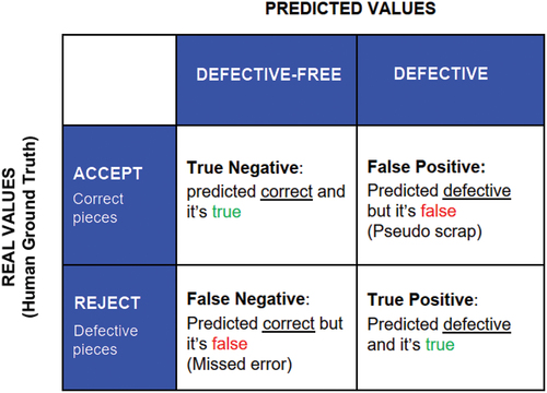
For the sake of comprehension, the terminology used hereinafter for the performance of defect detection systems is clarified below. The article (Mullany et al., 2022) is here used as a reference. Once the imperfections have been compared to the predetermined thresholds, the final step involves determining whether to ‘accept’ or ‘reject’ the part, which leads to the four options graphically summarized in Figure 1 (confusion matrix).

1. True Positive (TP).

2. False Negative (FN).

3. True Negative (TN).

4. False Positive (FP).

Figure 1. Confusion Matrix.

To evaluate the performance of a high-volume inspection or automated system, various metrics based on these four categories are utilized (see Table 1), which are reported as in (Mullany et al., 2022) as well.

Table 1. Summary of metrics used to assess the performance of a defect detection system.

Metric	Formula
Detection Success Rate	(TN+TP)/(TP+TN+FN+FP)
True Positive Accuracy	TP/(TP+FP)
True Positive Rate	TP/(TP+FN)
True Negative Rate	TN/(TN+FP)
True Negative Accuracy	TN/(TN+FN)
False Positive Rate	FP/(FN+TP)
False Negative Rate	FN/(FN+TP)

It is noteworthy that the 2D MVS acquire the light reflected from the surface of the object. Depending on the type of defect, the light is reflected highlighting the defect at a certain point. This works in the case of, for example, scratches, texture changes or colour changes (Cavaliere et al., 2022). Furthermore, they are sensitive to spurious reflections from overly reflective materials. An excessive amount of light can create an overexposed frame, which leads to light bleeding or blurred object edges, as has been observed in previous research (Cavaliere et al., 2021). The 3D MVS can use several technologies to generate 3D images of an object. Among them, laser triangulation (LT) evaluates the alteration of a laser beam when it is projected onto the object, using a camera having the optical axis inclined to the laser beam. LT requires continuous motion to capture a surface, which can be achieved with automated motion of the sensor around the object. It should be noted that LT is widely used in many fields due to its good stability, high resolution and speed. However, these applications suffer from limitations in data acquisition accuracy especially with curved surfaces as presented in (Dong et al., 2018).

Therefore, 3D MVS systems are best suited for cases where surface depth variations need to be measured, as well as for geometric and structural measurements.

In the following section, a case study will be presented for which there is evidence that the type of component analysed and the characteristic defect types lend themselves to being identified using both 2D and 3D systems. In these circumstances, based on the available MVS, the component should be subjected to a duplex inspection procedure using a 2D and a 3D system in series. To avoid duplex inspection and the consequent negative implications in terms of timing, ease of manipulation, need for space and sustainability, a bespoke combined 2D and 3D system has been developed. Furthermore, the following literature references have been taken into account as performance references for the application of Artificial Intelligence in quality control with similarities due to manufacturing processes or the use of image-based systems.

• In Papananias et al. (2020), the TP, as an index of the reduction of the number of parts to be inspected by humans, were 82% and 93% for a supervised and unsupervised system, respectively.

• In Bak et al. (2021), systems predicting incompliance of parts based on manufacturing parameters in die-casting applications performed with a Detection Success Rate of 99.5%, which can be assumed as a best-case scenario for standard applications that do not include MV.

• Different algorithms in Scime & Beuth (2018) showed performances between 85% and 97% in terms of Detection Success Rate through alternative image-based systems.

3. Presentation of a case study possibly benefitting from a hybrid machine vision system

3.1. Situations requiring 2D and 3D data for defect detection

As highlighted in the previous sections, the geometrical complexity, the typology and the position of surface defects are critical for the preference towards 2D or 3D MVS. The development of hybrid systems should target those parts possibly exhibiting a number of defects, where some can be captured by the former in a more straightforward way, while the identification of others requires the implementation of the latter.

3.2. Case study

A case in point is the component shown in Figure 2, which is the basis of the Long-Range Radar Sensor system that is part of the Advanced Driver-Assistance Systems in new-generation cars. The component has been used as a reference for the development and testing of the hybrid MVS. The datasets used for this study, which include this kind of component only, are presented in Section 4.

Figure 2. Aluminium die casting component chosen for the evaluation of surface defects: Figure (a) represents the raw analysed component, the subject of this study, Figure (b) represents the assembled component with all its parts ready to be installed on a car.

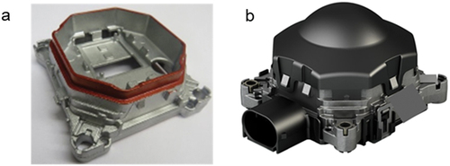
On request of a customer operating in the automotive industry, the component is currently manufactured by Alupress AG, a company specialised in the production of die-cast aluminium parts. Given the advances discussed in the introduction with regard to MVS, the company’s focus shifted to the use of AI in inspection systems and integration into the production process. This made it possible to conduct the current study at Alupress AG’s premises and use the component for the development and testing of the MVS. Industrial requirements were accordingly taken into account based on the company’s objectives.

3.3. Peculiar defects of the studied part and current performances of human inspection

As requested by the customer, all components have to be inspected after casting, moulding, slide grinding and before packaging. Skilled workers involved in the inspection of the specific aluminium component achieve a 90% true positive rate and a 10% false negative rate. The current human-based quality checks cover the entire component, i.e. the perimeter zone, the upper zone and the lower inner zone. Clearly, many types of defects can be detected; the most relevant ones for this case study are illustrated below in relation to customer requirements, which include geometric accuracy and technical cleanliness. The number of unidentified incompliances has to be minimized because surface defects can give rise to electronic malfunctions and incorrect assembly of the other parts that constitute the sensor.

Three types of defects were focused on, which are described in the numbered list that follows along with the area of the object where they are typically found (if applicable), and the MVS possibly more suitable to identify each defect separately.

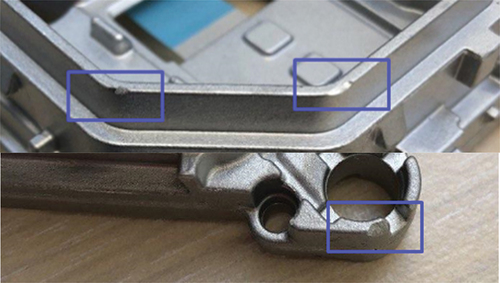
1. Burrs: they can be caused by material extending beyond the edges of the mould during the injection of molten aluminium. The presence of burrs is both unsightly and dangerous, as it can cause short circuits in the electronics and injuries to workers handling the metal parts during production. All the holes can be subject to burrs, as shown in Figure 3 through an illustrative example evidencing the position of the burr in the investigated part through an arrow and a blue circle (Figure 3a) and a magnified view of the defect highlighted by the blue box in Figure 3b. As for the analysed component, the detected burrs are generated during both the moulding of the component and the shearing and subsequent removal of the sprue and casting attachments from the mould itself. The size of these residual burrs on the component ranges from 0.4 mm to 2 mm. Components after burr removal are 100% accept parts, if no other critical defects are present. In Figure 4a, by means of the blue boxes, it is possible to observe the appearance of a burr along the perimeter surface at multiple geometry jumps generated by the bogies in the die-casting mould. The permissible burr size according to requirements is 600 µm (Figure 4b). Based on their typical morphology and orientation (orthogonal to holes), most of the burrs are expected to be present on horizontal surfaces; as regards these burrs, specific quality parameters are defined (by the customer). This is due to the manufacturing process and, specifically, to the geometric differences caused by the use of two different sliders belonging to the die. Burrs on horizontal surfaces are best identified and assessed by 2D systems. Other burrs with no specific quality criteria to consider can be tracked by a 3D system because of their orientation.

   Figure 3. Typical appearance of burrs: in Figure (a), the appearance of a burr on the perimeter edge, in Figure (b), a burr inside a hole.

   

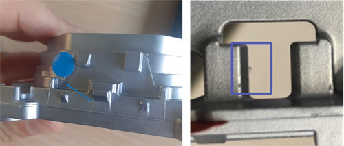
   Figure 4. a) Typical component burrs are shown on the left. b) the maximum permissible burr size according to the customer’s drawing is 600 µm.

   

2. Cold flow: this defect comprises a pre-solidified part of the material covered with an oxide layer to the later solidified melt caused by incorrect process control during casting. The defect is disconnected from the surrounding material and can be located all over the part close to the surface. In Figure 5, two examples of cold flow defects are shown and highlighted through blue boxes. The transition from the defect area to the surrounding material is rather sharp (strong gradient of grey/colour-level). This kind of defect is frequently located in heat sink zones. Any component with this defect is a Reject part in 100% of the cases. Because of their unpredictable positions, cold flow defects could be best identified through 3D MVS.

   Figure 5. Cold flow defects.

   

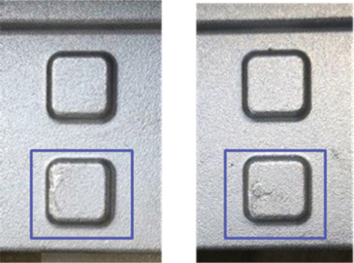
3. Breakouts: broken out material of sizes in the range of 0.5 mm to 15 mm. They can appear everywhere on the part, oftentimes at the circumference or protruding areas and render a component a Reject part in 100% of the cases. Illustrative breakouts are highlighted through blue boxes in Figure 6 for two different parts belonging to the same sample. Because of the difficulty to predict their location and orientation, 3D MVS have better chances to detect breakouts.

   Figure 6. Breakouts defects.

   

4. Methodology

The present section illustrates the methodological choices to develop the hybrid MVS. The three subsections in which it is articulated regard the DL approach, the hardware systems, and the architecture of the MVS, respectively. The development took place considering these three aspects contextually; hence, the process steps were conducted in parallel. The exigencies emerging from the case study were considered, but, at the same time, the authors took into account the generalizability of the approach and the adaptability of the MVS to other parts, situations and case studies. In this sense, the above case study can be seen as a trigger for the development of the system and any customization of the MVS is due to need to test it with a batch of the presented part.

4.1. Choice of the deep learning approach

Overall, the DAE network and other sophisticated approaches such as ResNet (Residual Networks) (Targ et al., 2016), and YOLO serve different purposes and excel in different areas. Based on literature (Hatab et al., 2021; Niu et al., 2021; Prunella et al., 2023), a comparison to understand their strengths and preferred applications is illustrated in Table 2.

Table 2. Characteristics and strengths of the DL architectures to be possibly considered for the development of the hybrid 2D-3D system.

ARCHITECTURE	DAE	ResNet	YOLO
Purpose	Primarily used for unsupervised learning tasks, particularly in image denoising and feature learning. •Aims to reconstruct an input (often noisy) by learning to map it to a clean output.	Designed for DL tasks, particularly in image recognition and classification. Introduces residual connections to address the vanishing gradient problem, allowing for very deep networks.	Specifically designed for real-time object detection. Frames object detection as a single regression problem, predicting bounding boxes and class probabilities directly from full images.
Strengths	Good at learning robust feature representations. Effective in scenarios with noisy data or where unsupervised pre-training is beneficial. Often used in anomaly detection by learning the normal pattern and identifying deviations.	Excels in image classification tasks. Provides state-of-the-art performance in many vision tasks due to its deep architecture. Used as a backbone for various tasks including object detection, segmentation, etc.	Extremely fast and suitable for real-time applications. Provides a good balance between speed and accuracy. Simplifies the object detection pipeline into a single neural network, making it efficient.
Common applications	Image denoising. Anomaly detection (e.g. identifying defective products by learning the ‘normal’ appearance). Feature extraction for downstream tasks.	Image classification. Object detection (when combined with other architectures). Image segmentation. General feature extraction in DL pipelines.	•Real-time object detection. •Applications requiring quick and accurate detection like autonomous driving, video surveillance, and robotics.

The detection of surface defects involves the identification of anomalies or irregularities on surfaces. Based on Table 2, Resnet will not be considered for this specific task. Table 3 explains how each approach deals with this task.

Table 3. Strengths and weaknesses of the architectures considered for the identification of surface defects.

ARCHITECTURE	DAE	YOLO
Strengths	Excellent for detecting anomalies as it can learn the ‘normal’ surface appearance and identify deviations.	Effective for detecting and localizing multiple defects in real-time. Can handle various types of defects in a single pass.
Limitations	Might not be as effective if the defects are very subtle. And the model cannot distinguish between noise and actual defects.	Might struggle with very small Or subtle defects if not adequately trained or if the defects are rare in the training set.

When considering different methods for surface defect detection, the choice of an approach can affect the effectiveness of the solution significantly. If the primary goal is to identify anomalies in a context where defects are relatively rare and the data is largely uniform, DAE results the most suitable option. DAEs excel at anomaly detection, making them ideal for scenarios where the presence of defects is infrequent and subtle variations in the data need to be identified. As a consequence, DAE was chosen as a reference approach for the development of the present system for defect recognition.

4.2. Tools needed for machine vision inspection

This subsection illustrates the design choices for the ‘hardware’ of the original inspection system. As more apparent below, these choices are based on the combination of scientific knowledge, requirements of the industrial application, availability of products in the market, and convenience.

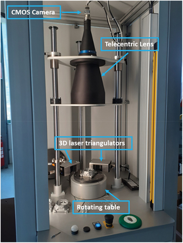
2D MVS is considered a mature technology (Steger et al., 2018) and many ready-to-use systems are available on the market. For this project, we chose to implement a state-of-the-art 2D MVS comprising a line-scan CMOS camera (5.1 Mpixel, 34.4 fps) equipped with a telecentric imaging system, with a depth of field of 111.3 mm and a working distance of 396 mm. The latter value allows the system to be used in a robotic cell and thus provides the necessary space for component handling. This favours the in-line application of the system, which ranges among the development requirements. The telecentric lens provides a constant magnification image of an object, facilitating calibration.

As mentioned in relation to the used component, the main objective of the 2D MVS is to detect burrs within the holes of the part. A backlight system was employed to highlight this type of defect. This method is normally used when it is necessary to detect through holes, when the object is overall opaque with variations of light and shadow in the areas of interest, or when it is necessary to outline its edges. The illumination is placed on the opposite side of the camera; the component is aligned with the light beam. The component is only recognisable as a silhouette and no assumptions can be made about the surface of the part. Because of this excessive light, the entire application is relatively resistant to stray light. In order to improve contrast and avoid collimation, telecentric backlighting was used. With this system, the backlight is perfectly aligned in parallel via a telecentric optical lens system.

For the 3D MVS, the choice was to use two 3D laser triangulators, arranged in such a way to avoid the shadow zones that can be generated due to the geometry of the part when passing the laser scan. The two 3D triangulators are oriented as shown in Figure 7, with a distance of 102 mm from the centre of the rotating platform.

Figure 7. (a) Measuring range of the 3D Laser Triangulators used; (b) 3D Laser Triangulators set up to capture the workpiece.

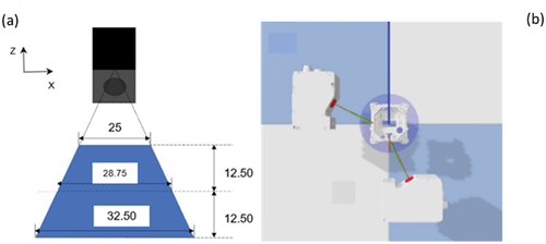
In the developed system, the maximum acquisition speed compatible with the laser triangulators to achieve the highest possible resolution is 1.7 kHz. The measuring range for the Z-axis (see Figure 7 for the arrangement of the coordinate system here and in the followings) is 25 mm and the Z resolution is 3 µm. The X resolution is 13–17 µm. The field of view is from 25.0 to 32.5 mm. The used processing software performs both CPU and GPU-based computations, with a multi-threaded architecture. The acquired point clouds are high-resolution data with approximately 50 million points. Thus, an 8 GB RAM is required to process them. The DL model runs on GPU for both training and deployment.

4.3. Architecture of the machine vision system

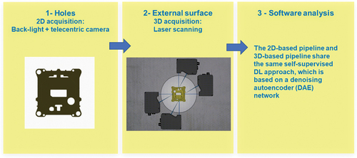
The developed automatic detection software consists of two pipelines concurring to identify surface defects through a measure of anomalies (Figure 8):

Figure 8. Workflow of the developed MVS where the two approaches for the 3D pipelines are the tested alternatives.

• a 2D-based pipeline to inspect the inner holes of the part;

• a 3D-based pipeline to inspect the lateral surfaces.

The two pipelines use different data sources (images and point clouds, respectively) and, consequently, different data processing techniques are implemented. After data acquisition, a pre-processing phase is performed to prepare raw 2D and 3D data for training and inference with the DAE network described below. The two pre-processing phases register raw 2D and 3D data to a reference template of the object. After registration, the data is presented to the network in a canonical, reference-centred view of the object, which greatly reduces the variability in the network input that arises from the variability in object location and pose under which data is acquired. Yet, as suggested in Figure 8, the 2D- and 3D-based pipelines share the same self-supervised DL approach, which works by means of the DAE network and a final classification step. This aspect, beyond being an element of originality for the developed MVS, is crucial to the reduction of processing times. The core idea is to learn the distribution of images of Accept parts, which are largely predominant in a production line, and then detect any deviation from this distribution occurring in defective pieces.

It is worth noting that, in light of the common approach for 2D and 3D data, separate results for the two different pipelines cannot be obtained, as the process works only when the results of both pipelines are combined.

The AE network is a reconstruction-based model and is trained in a self-supervised way, meaning that labelled data are not needed for learning. The AE has two main parts:

• an encoder that maps an input image into a lower dimensional representation (bottleneck), and

• a decoder that maps the bottleneck representation to a reconstruction of the input.

By minimizing the Mean Squared Error between input and output images, the network learns to reconstruct the input almost correctly. However, since the information needs to flow throughout the bottleneck, which is much smaller than the image, less frequent features are left out; as a result, anomalies might not be reconstructed. The higher the pixel-wise difference between input and output for a given patch, the likelier that the patch is anomalous. In addition, the DAE network corrupts the input images with a certain amount of noise (Gaussian noise, in this case) during training and learns to reconstruct the original undistorted input. This reduces overfitting and leads to a more robust learned representation. The developed network architecture is a fully convolutional AE based on the Residual Block (He et al., 2016), and, consequently, it automatically adapts to inputs at different resolutions.

The same DAE approach is applied with two types of data:

1. raw image for 2D data, and

2. as for 3D data, CAD distance image in a first approach, and surface gradient image in a second approach (see below).

After the reconstruction step, a final Accept/Reject score evaluation is assigned according to the process that follows. The difference between input and output, which can be interpreted as a heatmap showing differences in a graphical way, links each pixel with an anomaly score. The most common technique to provide a score for each image is summing all the anomaly scores for each pixel, e.g. (Chow et al., 2020). Eventually, a binary decision is needed: any piece that exceeds a threshold (usually chosen according to the validation set) is considered anomalous. While this simple rule might work if all anomalies are also defects, this is not always the case. For instance, dirt can be mistaken for a defect; for this reason, a final classification phase is used, which takes the heatmap as input to make decisions based on the structure of the anomaly heatmap. Then, the features are exploited to train a Multilayer Perceptron in a supervised manner and use it as the final classifier.

4.4. Details about pipelines and detection approaches

As far as the 2D pipeline is concerned, the acquired images are registered using an approach based on Generalised Hough Transform (GHT) (Ballard, 1981). First, a standard Canny edge detection is applied to each captured image, followed by a morphological filtering to clean spurious responses from the detection algorithm. The object pose is then found on the obtained edge binary image using template matching implemented as GHT. The reference template for GHT is first extracted from an edge binary image of the object, where the edge responses from the background have been manually cleaned. Given the location and pose of the object in the edge image found by GHT, the original image is reversely roto-translated to coincide with the template, and the object region is cropped around the template from the registered original image. The cropped image is first min-max normalized to the range [−1, 1]. The pixels in the cropped image corresponding to background in the template are set to a uniform value (zero, in our case). This step allows reducing the pixel-wise variability of the dataset and easily segmenting the background.

The 3D profiles are transformed into point clouds using the information about the displacement and orientation of the two sensors obtained in a calibration step, and the information about location and pose of the object obtained from the 2D images via the GHT. Since the frame rate of the laser sensors is higher than that of the camera on which the object location and pose are extracted, the information is up-sampled using interpolation. The point cloud obtained from the profiles of the object is then registered with the available CAD model of the component, used as a reference, by means of the Iterative Closest Point algorithm (Arun et al., 1987).

4.4.1. First 3D approach: CAD distance

In the first approach, after registration, a 2D map of displacements from the CAD model is then generated on a cylindrical image placed around the CAD model, by calculating the distance between the recorded 3D points and the CAD mesh. The displacement map is min-max normalized to the range [−1, 1]. It can be visualized as a greyscale image (Figure 9), which highlights any variation of the captured surface from the CAD surface.

Figure 9. Greyscale characterisation of analysed surface normal vectors.

4.4.2. Second 3D approach: surface gradient

Subsequently, due to the limitations found in this first 3D approach (see the results in the next section), a second approach concerning the surface gradient was tested.

In this case, the 3D profiles are again transformed into point clouds, but, here, the CAD is no longer used as a reference model. In this second approach, all normal vectors of the scanned surface are calculated. The normal axes are determined as those exiting the external surface of the reconstructed model based on the acquired point cloud and locally orthogonal to it. After that, the angle of inclination of the normal with respect to the corresponding orthogonal axis on the CAD model is calculated. The more inclined the vector is with respect to the vertical, the clearer it is in the greyscale image, see the example of Figure 9. Otherwise said, the α angle varies between 0 and π, while the clearest areas of Figure 10 are those associated with high α values where the most sudden curvature changes are located. Those are also the areas where defects are most likely to be found and which will be considered in the residual of the procedure.

Figure 10. MVS 2D-3D hybrid configuration.

4.4.3. Transformation of 3D point clouds into 2D images

The algorithm used to transform a 3D point cloud into a 2D image is known as ‘3D to 2D Projection’ or ‘3D Projection’. This technique involves projecting the 3D points onto a 2D plane to create a representation of the point cloud in two dimensions (Kaminsky et al., 2009). The orthographic projection was used as projection method, similarly to (Rong & Shen, 2023).

The accuracy enabled by orthographic projections is especially beneficial for quantitative analyses and measurements, ensuring that the data extracted from the images remains reliable. Furthermore, the simplified representation offered by orthographic projections can be advantageous for specific types of analysis and visualization tasks. By eliminating the complexities of perspective distortion, these images allow for easier identification of geometric relationships and symmetries within the scene, e.g. (Jovančević et al., 2017).

4.5. Implementation of the hybrid machine vision system

The configuration of the 2D and 3D instrumentation is integrated into a single solution (see Figure 10), which includes a metal support structure where the camera is installed on a telecentric lens. The movement of components during image acquisition and subsequent analysis is performed by a rotating table, under which the backlight is located. The component is positioned correctly thanks to a centring mask. Pick-and-place is performed by an industrial robot installed in the production cell, whose movements have been optimised to achieve the best possible cycle time.

The metal frame including all elements is equipped with panels around the acquisition sensors that prevent any variation in external light from affecting the acquisition process. In addition to determining the position of the rotating table, the incremental encoder communicates this information to the laser triangulators. In this way, the correct information about the position of the component is provided to all sensing instruments used for analysis.

Moving the component with the rotating table reduces noise and motion interference introduced by the robotic arm, which is a much more complex system with many degrees of freedom and it is therefore more prone to oscillations during movement.

The 3D laser triangulators are arranged around the rotating table. The position angle of the rotating table is adjusted via an incremental encoder. Such information is synchronised with the start-and-stop of the triangulators. A schematic description of the various steps described above is shown in Figure 11.

Figure 11. Schematic diagram of image acquisition and processing by the MVS 2D-3D.

4.6. Training of the deep learning model and output data

The model has been trained with the images of 1200 Accept components (training set). Subsequently, the model attempts to reconstruct the images with a difference between the actual images and the images reconstructed from the DL model. Eventually, the heatmap is calculated and the anomaly score is then computed in line with the steps typically followed in DL algorithms (Samek et al., 2016), see Figure 8, bottom part.

More in details, the training set has been handled in line with Figure 12. Data preparation is the process of selecting the right data to build a training set from original data and making data suitable for DL. The original data may require a number of pre-processing steps to transform the raw data before training and validation sets can be extracted, for example the transformation of the 3D point cloud into a 2D raw image. Pre-processing steps can include cropping to isolate features of interest, extracting small datasets from marked slices, and filtering to enhance images. Training sets include the training input(s) and output(s), as well as an optional mask(s) and validation set. During training, models are fit to parameters in a process that is known as adjusting weights.

Figure 12. Flowchart depicting the management of the training plot and other data to train and fine tune the DL architecture.

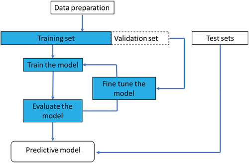
The test data set is used to evaluate the goodness of the predictive model previously trained with the training set. In DL projects, the training set cannot be used in the testing stage because the algorithm would already know in advance the expected output.

5. Results and discussion

The following collection of data (Datasets) were used to test and evaluate the performance of the DL algorithm:

• Dataset 1: 260 Accept parts + 200 Reject parts

• Dataset 2: 100 Accept parts + 100 Reject parts

• Dataset 3: 140 Accept parts + 37 Reject parts

All components belonging to all Datasets were manufactured with the same mould, but each dataset differs in terms of its manufacturing period. The Datasets are ordered according to their increasing age of the mould at the time of manufacturing.

5.1. Results

All the data that follows apply to the combination of the three datasets.

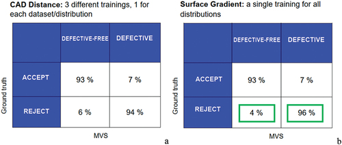
As can be seen in Figure 13, the percentage of FN dropped from 6% to 4% and, accordingly, the percentage of TP rose from 94% to 96% by switching from the CAD Distance to the Surface Gradient approach. Details follow.

Figure 13. Difference in values between Confusion Matrices for the CAD Distance approach (a) and the Surface Gradient approach (b). The percentage of FN and TP are highlighted.

Slight geometrical differences are typically found on parts produced in different months although with the same mould, which distinguishes the three datasets. This is embodied in slight deviations across parts in terms of hundredths of millimetres, which can occur due to the slight interference in the closing of the moving parts of the mould, such as the sliders. This concept is made evident in Figure 14, where the graph represents the variability (in millimetres) of certain areas of the component. Each profile is represented by a horizontal line on the image and the values on the ordinates are the depth values corresponding to each pixel on the line.

Figure 14. Geometric variability related to the geometry of the pieces of the same the die-casting mould.

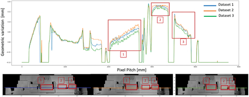
Three significant areas have been highlighted where this variation can be observed in relation to parts produced with the same mould at different times. Differences in depth at the same geometric position (highlighted in red, 1, 2, and 3) of 0.05–0.06 mm can be observed. Such variations are physiological and acceptable for a die-casting process, but troublesome when being analysed with an automatic DL-based system, which makes the validation of the effectiveness and stability of the algorithm challenging. The first 3D approach turned to suffer from these issues, i.e. it exhibited problems in distinguishing the mentioned variations and imperfections to be actually considered as surface defects.

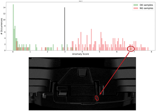
With the second approach, the difficulty of recognising surfaces characterised by the inherent geometric variability of the production process is significantly reduced. In some of the samples analysed, the system detected defect-free areas when the defect was present. Through the histogram in Figure 15, the distribution of anomaly scores is shown, while the green and red colours are intended to denote Accept parts and Reject parts, respectively. While it is possible to observe that the majority of Accept parts are characterized by low anomaly scores and Reject parts are mostly found on the right-hand side of the histogram, exceptions are still diffused. The most notable error in terms of FN is illustrated in the bottom area of Figure 15. For a better reading of Figure 15, it is worth noting here that the threshold assigned by the system to discriminate Accept parts Reject parts was approximately 3. Therefore, an ideal outcome of the application of the MVS would be to find all green (red) bars on the left (right) of the reported black vertical line.

Figure 15. Graphical output of a FN part through an unidentified defect (illustration below) and its correspondence in the distribution of occurrences of parts classified on anomaly scores (histogram above).

5.2. Discussion

The above results are the product of the hybridization of 2D and 3D-based systems supported by the MV technology. The targets set forth in the introduction have been reached. The unique combination proposed here has allowed the recognition of different defects, which could have not taken place by the 2D camera and 3D triangulators alone in their current configuration. To inspect all defects, a larger number of cameras would have been required, but this would have not enabled the acquisition of data suitable for future defect measurement, which is included in authors’ future work beyond the interests of the company.

The presented results were considered satisfactory by the company, while it is problematic to compare them with alternative automatic defect detection systems, as aforementioned. This is due to the fact that the used MVS is bespoke, although the used approach can be generalized, and original in methodological terms. If the attention is shifted to the broader field of the use of Artificial Intelligence in quality control, the here presented MVS is in line or outperforms the image-based systems illustrated in the second section, while the targets of prediction systems cannot be overcome.

The outcomes are acceptable especially in consideration of the limited number of FN, which represent a major problem for manufacturing companies in terms of possible complaints. The reduction of FN from 6% to 4%, which has taken place thanks to the introduction of the Surface Gradient approach, can be considered as the reaching of an important target according to the aims of the involved company. Obviously, the superiority of the second-attempt approach should be verified with other case studies. It is also noteworthy that these results are limited by the availability of parts produced with a single mould, while the production of large die-cast batches could require additional moulds. The stability of the results in the event of changing the mould should be verified.

As an additional output, the time required for the inspection of parts with the MVS is in line with the human-based tasks that are currently performed – more precise data in this regard cannot be disclosed because of confidentiality. As regards time efficiency, a validation of the developed system has to be made with parts characterized by different geometries and kinds of defects. This calls into question the flexibility of the system in terms of new parts to subject to the tests, which could clearly vary according to multiple aspects. Based on acquired experience, below is the authors’ view on the stability of the system according to possible changes.

• Component size: the same approach can be used, the acquisition system needs to be changed (size of the roundtable, distance of the telecentric from the component).

• Features and defects: the same approach can be used, the need arises to redo the training; in HPDC, typologies and defects are substantially equivalent across parts.

• Material and appearance: the same approach can be used, reflectivity and consequently light parameters are to be considered and adapted; images should be of the highest quality possible.

6. Conclusions

This article presents the development of a hybrid 2D/3D MVS for the detection of surface defects in die-cast aluminium components. The combination was deemed necessary and convenient for a case study in the automotive industry where the nature and position of defects are various. This situation is common in industrial settings where high quality standards are in place. The research objectives have been pursued in that:

• The hybridisation of 2D and 3D data sources has taken place by transforming 3D cloud points through specific algorithms and analysing the outcomes conjointly with 2D images in a single DL environment. This solution, enabled by the DAE DL algorithm, has prevented a serialised use of 2D- and 3D-based MVS, which would have increased processing time.

• The accuracy (for both TP and TN) of the MVS outperformed the set threshold of 90% with two different 3D pipelines. The results achieved through the use of Surface gradient were particularly appreciable as the number of true negatives, which were in focus, increased.

• While the results are fully comparable with human inspection, the time for processing has been reduced. The introduction of an automatic system to replace human tasks is set to be more robust and less dependent on human concentration. The time needed by the hybrid system to operate and the integrated components and actuators (Fig. 8) make the system usable in-line. In this regard, it is worth noting that the software environment not only enables defect detection, but also provides for the management of and communication between the hardware components. Moreover, the system manages both the actuators of the rotating table and the coordination of start-and-stop signals of the robot integrated in the cell illustrated in Fig. 8.

In this configuration of the developed system, the major task to be performed by experts is to establish the defects to be designated to the 2D and 3D pipelines beyond supervising the training operations and choosing the necessary Accept and Reject parts for the training itself. In the present case, it has been decided to process burrs with the 2D technology, as the task is relatively easy and no sophisticated data elaboration is required. On the other hand, the outline of the part required the use of the 3D system because of its complexity. In addition, the designer of the analysed part intends to introduce automatic systems for the measurement of defects. As such, a perspective development of the MVS is to use acquired data for measurement and to test the usability of anomaly scores for the same purpose.

The authors consider the developed MVS as an important research outcome once its performances can be generalized. To this aim, future work includes its adaptation for other parts and testing of its accuracy in different circumstances. This is enabled by the fact that customised DL applications were used, and adaptations are therefore both possible and needed. These further developments making the system adaptable for any component have to be followed by ablation studies to optimize and enhance the final algorithm performance through the removal of unnecessary components and the consequent reduction of algorithm complexity.

From an industrial viewpoint, an important goal was the simplification and reduction of human-based activities, typically frustrating and prone to errors. Using this system in the specific organisation’s context, the role of operators currently tasked with visual inspection will be limited to the rework of components to mechanically remove some defects, e.g. as in presence of burrs. These operators will also take the final decision for those components that the system was unable to identify as compliant or uncompliant.

Despite the progress made, this work still faces limitations and unresolved issues, which lead to the need for further research and exploration.

First, expanding the scope of tests to encompass a wider range of configurations and a greater number of parts will contribute to improving the learning capabilities of the system. By using the DL model with different parts and characteristic surface defects, the system can prove its effectiveness. In particular, expanding the testing to include other automotive components will provide a more comprehensive evaluation of the system applicability. By assessing its performance on different types of components, the system versatility and adaptability can be verified, enabling its potential deployment in various manufacturing processes. A capability test of the measuring and testing processes is crucial to validate the system’s performance based on the 6σ-based guidelines. This validation step ensures the reliability and accuracy of the system’s measurements, further bolstering its capability to identify anomalies. To enhance productivity and reduce cycle time, the implementation of two additional laser triangulators will be tested. This expansion aims to streamline the inspection process, allowing for simultaneous measurements and thereby increasing the throughput of the system.

Moreover, investigating the relationship between anomaly scores and categories of defects might facilitate the identification of severe problems and, possibly, the specific issues that may arise during manufacturing processes. This research direction can enable a deeper understanding of the underlying causes behind anomalies, leading to more targeted and effective quality control measures.

Acknowledgement

This work was supported by the Open Access Publishing Fund of the Free University of Bozen-Bolzano.

Disclosure statement

No potential conflict of interest was reported by the author(s).

References

- Ali, M. A., & Lun, A. K. (2019). A cascading fuzzy logic with image processing algorithm–based defect detection for automatic visual inspection of industrial cylindrical object’s surface. International Journal of Advanced Manufacturing Technology, 102(1–4), 81–28. https://doi.org/10.1007/s00170-018-3171-7
- Arun, S., Huang, T. S., Blostein, S. D. (1987). Least-square fitting of two 3-D point sets. IEEE Transactions on Pattern Analysis & Machine Intelligence, 9(5), 698–700. https://doi.org/10.1109/TPAMI.1987.4767965
- Badmos, O., Kopp, A., Bernthaler, T., & Schneider, G. (2020). Image-based defect detection in lithium-ion battery electrode using convolutional neural networks. Journal of Intelligent Manufacturing, 31(4), 885–897. https://doi.org/10.1007/s10845-019-01484-x
- Bak, C., Roy, A. G., & Son, H. (2021). Quality prediction for aluminum diecasting process based on shallow neural network and data feature selection technique. CIRP Journal of Manufacturing Science and Technology, 33, 327–338. https://doi.org/10.1016/j.cirpj.2021.04.001
- Ballard, D. H. (1981). Generalizing the Hough transform to detect arbitrary shapes. Pattern Recognition, 13(2), 111–122. https://doi.org/10.1016/0031-3203(81)90009-1
- Bharambe, C., Jaybhaye, M. D., Dalmiya, A., Daund, C., & Shinde, D. (2023). Analyzing casting defects in high-pressure die casting industrial case study. Materials Today: Proceedings, 72, 1079–1083. https://doi.org/10.1016/j.matpr.2022.09.166
- Bulnes, F. G., Usamentiaga, R., Garcia, D. F., & Molleda, J. (2016). An efficient method for defect detection during the manufacturing of web materials. Journal of Intelligent Manufacturing, 27(2), 431–445. https://doi.org/10.1007/s10845-014-0876-9
- Cavaliere, G., Borgianni, Y., & Rampone, E. (2022). Development of a system for the analysis of surface defects in die-cast components using machine vision. In D, T. Matt, R. Vidoni, E. Rauch, & P. Dallasega (Eds.), Managing and Implementing the Digital Transformation. ISIEA 2022 (Vol. 525, pp. 74–86). Springer, Cham: Lecture Notes in Networks and Systems. https://doi.org/10.1007/978-3-031-14317-5_7
- Cavaliere, G., Borgianni, Y., & Schäfer, C. (2021). Study on an in-line automated system for surface defect analysis of aluminium die-cast components using artificial intelligence. Acta Technica NapocenActa Technica Napocensis Series Applied Mathematics, Mechanics and Engineeringsis, 64(3), 475–486.
- Chow, J. K., Su, Z., Wu, J., Tan, P. S., Mao, X., & Wang, Y. H. (2020). Anomaly detection of defects on concrete structures with the convolutional autoencoder. Advanced Engineering Informatics, 45, 101105. https://doi.org/10.1016/j.aei.2020.101105
- DiLeo, G., Liguori, C., Pietrosanto, A., & Sommella, P. (2017). A vision system for the online quality monitoring of industrial manufacturing. Optics and Lasers in Engineering, 89, 162–168. https://doi.org/10.1016/j.optlaseng.2016.05.007
- Dong, Z., Sun, X., Liu, W., & Yang, H. (2018). Measurement of free-form curved surfaces using laser triangulation. Sensors, 18(10), 3527. https://doi.org/10.3390/s18103527
- Duan, L., Yang, K., & Ruan, L. (2020). Research on automatic recognition of casting defects based on deep learning. Institute of Electrical and Electronics Engineers Access, 9, 12209–12216. https://doi.org/10.1109/ACCESS.2020.3048432
- Goodfellow, I., Pouget-Abadie, J., Mirza, M., Xu, B., Warde Farley, D., Ozair, S., Courville, A., & Bengio, Y. (2014). Generative adversarial nets. Advances in Neural Information Processing Systems, 27.
- Gu, J., Wang, Z., Kuen, J., Ma, L., Shahroudy, A., Shuai, B., Liu, T., Wang, X., Wang, G., Cai, J., & Chen, T. (2018). Recent advances in convolutional neural networks. Pattern Recognition, 77, 354–377. https://doi.org/10.1016/j.patcog.2017.10.013
- Guo, Y., Wang, H., Hu, Q., Liu, H., Liu, L., & Bennamoun, M. (2020). Deep learning for 3d point clouds: A survey. IEEE Transactions on Pattern Analysis & Machine Intelligence, 43(12), 4338–4364. https://doi.org/10.1109/TPAMI.2020.3005434
- Hatab, M., Malekmohamadi, H., & Amira, A. (2021). Surface defect detection using YOLO network. Intelligent Systems and Applications: Proceedings of the 2020 Intelligent Systems Conference (IntelliSys) Volume 1, 3-4 September 2020, London, UK (pp. 505–515). Springer International Publishing.
- He, K., Zhang, X., Ren, S., & Sun, J. (2016). Deep residual learning for image recognition. Proceedings of the IEEE conference on computer vision and pattern recognition, 20-25 June 2009, Miami, FL (pp. 770–778).
- Hinton, G. E., & Salakhutdinov, R. R. (2006). Reducing the dimensionality of data with neural networks. Science, 313(5786), 504–507. https://doi.org/10.1126/science.1127647
- Jia, H., & Liu, W. (2023). Anomaly detection in images with shared autoencoders. Frontiers in Neurorobotics, 16, 1046867. https://doi.org/10.3389/fnbot.2022.1046867
- Jones, C. W., & O’Connor, D. (2018). A hybrid 2D/3D inspection concept with smart routing optimisation for high throughput, high dynamic range and traceable critical dimension metrology. Measurement Science and Technology, 29(7), 074004. https://doi.org/10.1088/1361-6501/aababd
- Jovančević, I., Pham, H. H., Orteu, J. J., Gilblas, R., Harvent, J., Maurice, X., & Brèthes, L. (2017). 3D point cloud analysis for detection and characterization of defects on airplane exterior surface. Journal of Nondestructive Evaluation, 36(4), 1–17. https://doi.org/10.1007/s10921-017-0453-1
- Kaminsky, R. S., Snavely, N., Seitz, S. M., & Szeliski, R. (2009, June). Alignment of 3D point clouds to overhead images. 2009 IEEE computer society conference on computer vision and pattern recognition workshops, 20-25 June 2009, Miami, FL (pp. 63–70). IEEE.
- Kim, D. H., Kim, T. J., Wang, X., Kim, M., Quan, Y. J., Oh, J. W., Min, S. H., Kim, H., Bhandari, B., Yang, I., & Ahn, S. H. (2018). Smart machining process using machine learning: A review and perspective on machining industry. International Journal of Precision Engineering and Manufacturing-Green Technology, 5(4), 555–568. https://doi.org/10.1007/s40684-018-0057-y
- Liu, L., Ouyang, W., Wang, X., Fieguth, P., Chen, J., Liu, X., & Pietikäinen, M. (2020). Deep learning for generic object detection: A survey. International Journal of Computer Vision, 128(2), 261–318. https://doi.org/10.1007/s11263-019-01247-4
- Liu, X., Zhou, Q., Zhao, J., Shen, H., & Xiong, X. (2019). Fault diagnosis of rotating machinery under noisy environment conditions based on a 1-D convolutional autoencoder and 1-D convolutional neural network. Sensors, 19(4), 972. https://doi.org/10.3390/s19040972
- Malamas, E. N., Petrakis, E. G., Zervakis, M., Petit, L., & Legat, J.-D. (2003). A survey on industrial vision systems, applications and tools. Image and Vision Computing, 21(2), 171–188. https://doi.org/10.1016/S0262-8856(02)00152-X
- Mery, D. (2020). Aluminum casting inspection using deep learning: A method based on convolutional neural networks. Journal of Nondestructive Evaluation, 39(1), 12. https://doi.org/10.1007/s10921-020-0655-9
- Mullany, B., Savio, E., Haitjema, H., & Leach, R. (2022). The implication and evaluation of geometrical imperfections on manufactured surfaces. CIRP Annals, 71(2), 717–739. https://doi.org/10.1016/j.cirp.2022.05.004
- Nikolić, F., Štajduhar, I., & Čanađija, M. (2023). Casting defects detection in aluminum alloys using deep learning: A classification approach. International Journal of Metalcasting, 17(1), 386–398. https://doi.org/10.1007/s40962-022-00777-x
- Niu, T., Li, B., Li, W., Qiu, Y., & Niu, S. (2021). Positive-sample-based surface defect detection using memory-augmented adversarial autoencoders. IEEE/ASME Transactions on Mechatronics, 27(1), 46–57. https://doi.org/10.1109/TMECH.2021.3058147
- Ördek, B., Borgianni, Y., & Coatanea, E. (2024). Machine learning-supported manufacturing: A review and directions for future research. Production and Manufacturing Research, 12(1), 2326526. https://doi.org/10.1080/21693277.2024.2326526
- Papananias, M., McLeay, T. E., Obajemu, O., Mahfouf, M., & Kadirkamanathan, V. (2020). Inspection by exception: A new machine learning-based approach for multistage manufacturing. Applied Soft Computing, 97, 106787. https://doi.org/10.1016/j.asoc.2020.106787
- Parlak, İ. E., & Emel, E. (2023). Deep learning-based detection of aluminum casting defects and their types. Engineering Applications of Artificial Intelligence, 118, 105636. https://doi.org/10.1016/j.engappai.2022.105636
- Penumuru, D. P., Muthuswamy, S., & Karumbu, P. (2019). Identification and classification of materials using machine vision and machine learning in the context of industry 4.0. Journal of Intelligent Manufacturing, 31(5), 1229–1241. https://doi.org/10.1007/s10845-019-01508-6
- Pérez, L., Rodríguez, Í., Rodríguez, N., Usamentiaga, R., & García, D. F. (2016). Robot guidance using machine vision techniques in industrial environments: A comparative review. Sensors, 16(3), 335. https://doi.org/10.3390/s16030335
- Prunella, M., Scardigno, R. M., Buongiorno, D., Brunetti, A., Longo, N., Carli, R., Dotoli, M., & Bevilacqua, V. (2023). Deep learning for automatic vision-based recognition of industrial surface defects: A survey. Institute of Electrical and Electronics Engineers Access, 11, 43370–43423. https://doi.org/10.1109/ACCESS.2023.3271748
- Qi, C. R., Su, H., Mo, K., & Guibas, L. J. (2017). Pointnet: Deep learning on point sets for 3d classification and segmentation. Proceedings of the IEEE conference on computer vision and pattern recognition, 21-26 July 2017, Honolulu, HI, USA (pp. 652–660).
- Qi, S., Yang, J., & Zhong, Z. (2020). A review on industrial surface defect detection based on deep learning technology. Proceedings of the 2020 3rd International Conference on Machine Learning and Machine Intelligence, 18-20 September 2020, Hangzhou, China (pp. 24–30).
- Rahimi, A., Anvaripour, M., & Hayat, K. (2021, June). Object detection using deep learning in a manufacturing plant to improve manual inspection. 2021 IEEE International Conference on Prognostics and Health Management (ICPHM), 7-9 June 2021, Detroit, MI (pp. 1–7). IEEE.
- Ren, Z., Fang, F., Yan, N., & Wu, Y. (2022). State of the art in defect detection based on machine vision. International Journal of Precision Engineering and Manufacturing-Green Technology, 9(2), 661–691. https://doi.org/10.1007/s40684-021-00343-6
- Rong, M., & Shen, S. (2023). 3D Semantic segmentation of aerial photogrammetry models based on orthographic projection. IEEE Transactions on Circuits and Systems for Video Technology, 33(12), 7425–7437. https://doi.org/10.1109/TCSVT.2023.3273224
- Rumelhart, D. E., Hinton, G. E., & Williams, R. J. (1986). Learning representations by back-propagating errors. Nature, 323(6088), 533–536. https://doi.org/10.1038/323533a0
- Samek, W., Binder, A., Montavon, G., Lapuschkin, S., & Müller, K. R. (2016). Evaluating the visualization of what a deep neural network has learned. IEEE Transactions on Neural Networks and Learning Systems, 28(11), 2660–2673. https://doi.org/10.1109/TNNLS.2016.2599820
- Savio, E., De Chiffre, L., Carmignato, S., & Meinertz, J. (2016). Economic benefits of metrology in manufacturing. CIRP Annals, 65(1), 495–498. https://doi.org/10.1016/j.cirp.2016.04.020
- Schlegl, T., Seeböck, P., Waldstein, S. M., Langs, G., & Schmidt-Erfurth, U. (2019). f-AnoGAN: Fast unsupervised anomaly detection with generative adversarial networks. Medical Image Analysis, 54, 30–44. https://doi.org/10.1016/j.media.2019.01.010
- Schöch, A., Salvadori, A., Germann, I., Balemi, S., Bach, C., Ghiotti, A., Carmignato, S., Maurizio, A. L., & Savio, E. (2015). High-speed measurement of complex shaped parts at elevated temperature by laser triangulation. International Journal of Automation Technology, 9(5), 558–566. https://doi.org/10.20965/ijat.2015.p0558
- Scime, L., & Beuth, J. (2018). A multi-scale convolutional neural network for autonomous anomaly detection and classification in a laser powder bed fusion additive manufacturing process. Additive Manufacturing, 24, 273–286. https://doi.org/10.1016/j.addma.2018.09.034
- Sharifzadeh, S., Biro, I., Lohse, N., & Kinnell, P. (2018). Abnormality detection strategies for surface inspection using robot mounted laser scanners. Mechatronics, 51, 59–74. https://doi.org/10.1016/j.mechatronics.2018.03.001
- Silva, R. L., Rudek, M., Szejka, A. L., & Junior, O. C. (2018, July 2–4). Machine vision systems for industrial quality control inspections. Product lifecycle management to support Industry 4.0: 15th IFIP WG 5.1 International Conference, PLM 2018, Proceedings 15, July 2–4, 2018, Turin, Italy (pp. 631–641). Springer International Publishing.
- Song, K., & Yan, Y. (2013). A noise robust method based on completed local binary patterns for hot-rolled steel strip surface defects. Applied Surface Science, 285, 858–864. https://doi.org/10.1016/j.apsusc.2013.09.002
- Steger, C., Ulrich, M., & Wiedemann, C. (2018). Machine vision algorithms and applications. John Wiley & Sons.
- Tan, X., & Triggs, B. (2007). Fusing Gabor and LBP feature sets for kernel based face recognition under difficult lighting conditions. Analysis and Modeling of faces and gestures. Lecture Notes in Computer Science, 4778, 168–182. https://doi.org/10.1007/978-3-540-75690-3_18
- Tang, B., Chen, L., Sun, W., & Lin, Z. K. (2023). Review of surface defect detection of steel products based on machine vision. IET Image Processing, 17(2), 303–322. https://doi.org/10.1049/ipr2.12647
- Targ, S., Almeida, D., & Lyman, K. (2016). Resnet in resnet: Generalizing residual architectures. arXiv Preprint arXiv: 160308029.
- Vincent, P., Larochelle, H., Bengio, Y., & Manzagol, P. A. (2008, July). Extracting and composing robust features with denoising autoencoders. Proceedings of the 25th International Conference on Machine learning, 5-9 July 2008, Helsinki, Finland (pp. 1096–1103.
- Wang, J., Fu, P., & Gao, R. X. (2019). Machine vision intelligence for product defect inspection based on deep learning and Hough transform. Journal of Manufacturing Systems, 51, 52–60. https://doi.org/10.1016/j.jmsy.2019.03.002
- Wang, T., Chen, Y., Qiao, M., & Snoussi, H. (2018). A fast and robust convolutional neural network-based defect detection model in product quality control. International Journal of Advanced Manufacturing Technology, 94(9–12), 3465–3471. https://doi.org/10.1007/s00170-017-0882-0
- Wu, Y., Qin, Y., Wang, Z., & Jia, L. (2018). A UAV-based visual inspection method for rail surface defects. Applied Sciences, 8(7), 1028. https://doi.org/10.3390/app8071028
- Xu, H., & Huang, Z. (2021). Annotation-free defect detection for glasses based on convolutional auto-encoder with skip connections. Materials Letters, 299, 130065. https://doi.org/10.1016/j.matlet.2021.130065
- Yan, Z., Shi, B., Sun, L., & Xiao, J. (2020). Surface defect detection of aluminum alloy welds with 3D depth image and 2D gray image. International Journal of Advanced Manufacturing Technology, 110(3–4), 741–752. https://doi.org/10.1007/s00170-020-05882-x
- Ye, J., Stewart, E., & Roberts, C. (2019). Use of a 3D model to improve the performance of laser-based railway track inspection. Proceedings of the Institution of Mechanical Engineers, Part F: Journal of Rail & Rapid Transit, 233(3), 337–355. https://doi.org/10.1177/0954409718795714
- Yue, Y., Finley, T., Radlinski, F., & Joachims, T. (2007). A support vector method for optimizing average precision. Proceedings of the 30th Annual International ACM SIGIR Conference on Research and Development in Information Retrieval, 23-27 July 2007, Amsterdam, The Netherlands (pp. 271–278.
- Zheng, X., Zheng, S., Kong, Y., & Chen, J. (2021). Recent advances in surface defect inspection of industrial products using deep learning techniques. International Journal of Advanced Manufacturing Technology, 113(1–2), 35–58. https://doi.org/10.1007/s00170-021-06592-8