Scheduling method of wind power generation for electricity market using state-of-charge transition and forecast error

ABSTRACT

This study focuses on the trade of power from wind power plants (WPPs) at an electricity market. To trade power, operators should produce generation schedules for bids and then supply the same amount of energy as the schedules. However, power from WPPs tends to fluctuate, which complicates scheduling. This paper proposes three scheduling methods with an energy storage system (ESS) to solve this problem. The first method considers state-of-charge (SOC) transition to maintain the appropriate SOC and minimize the imbalance between supplied and scheduled energy. The second and third methods consider SOC transition and forecast errors. The second method uses a linear regression model to estimate forecast errors. The third method adopts a bagged trees model, which is a machine learning method, to directly estimate the adjusted forecast data considering errors. Five patterns of the rated power of the ESS are assumed, and these three methods are simulated on each power. In comparison with the basic method, whose schedules are the same as the forecast, the third method can reduce 84% of the imbalance from the schedules when the rated power of the ESS is the minimum. The proposed methods help develop further correct and practical scheduling methods.

KEYWORDS:

• Energy storage system
• forecast error
• generation scheduling
• machine learning
• state-of-charge transition
• wind power

1. Introduction

A wind power generation system does not emit carbon dioxide and is effective for preventing global warming. However, power from wind power plants (WPPs) tends to fluctuate and is difficult to supply steadily, because wind, as the power source, is easily changed. Therefore, wind power generation cannot simply replace other existing generation methods, for example, thermal, nuclear, and hydroelectric power generation. Thus, various countries have introduced the renewable portfolio standard and/or the feed-in tariff (FIT) to promote the utilization of renewable energies, such as power from WPPs [1]. Currently, power from renewable energies can be sold at a fixed price under the FIT in Japan. However, the FIT will end in the near future, after which renewable energy operators may need to trade generated power at an electricity market. To trade this power, all operators must produce a generation schedule for bids and supply the same amount of energy as the schedule.

Approaches for producing generation schedules have been suggested [2–4]. Reference [2] proposed a bidding strategy where wind farms offer energy jointly compared with bidding strategies that consider each wind farm separately. Reference [3] proposed a bidding strategy by using a non-cooperative game approach based on bi-level optimization with utility companies and power producers of thermal, solar, and wind power. Reference [4] proposed a bidding strategy based on a stochastic linear mathematical programming to maximize profit.

Power from WPPs is difficult to forecast due to fluctuation. Thus, the generation schedule following the forecast tends to differ from the actual output of WPPs, and the imbalance will occur. Using an energy storage system (ESS) is an effective solution for minimizing the imbalance. The ESS can charge and discharge to coincide the actual output with the generation schedule. However, the state-of-charge (SOC) of the ESS should be considered because the ESS cannot charge or discharge when the SOC reaches 1 or 0. Therefore, the appropriate SOC should be maintained by optimizing generation schedules. Moreover, the SOC transition is a key factor for maintaining the appropriate SOC. Reference [5] developed a scheduling method with ESS and analysed economic feasibility. Considering forecast errors is another solution because these errors result in the imbalance. Reference [6] estimated the costs caused by forecast errors of wind generation in the market. Reference [7] focused on the uncertainty of price and wind power generation and proposed a bidding strategy using robust optimization with ESS. Reference [8] proposed rolling optimization models that consider forecast errors with the ESS for bidding and real-time control. Reference [9] focused on the partition of ESS power and energy capacity and developed a scheduling method that considers forecast errors with the ESS. However, scheduling methods that consider the SOC transition and forecast errors to maintain the appropriate SOC and minimize the imbalance should be further studied.

Our team has developed scheduling methods that consider the SOC transition [10,11]. The present study proposes and compares three scheduling methods to maintain the appropriate SOC and minimize the imbalance. The first method considers the SOC transition. The second and third methods consider the SOC transition and forecast errors. Forecast errors are estimated and forecast data are adjusted by using the estimated errors in the second method. In the third method, the adjusted forecast data considering errors are estimated directly. This study assumes a wind farm consisting of wind turbines and the ESS, and simulation is performed. The degree of imbalance from the generation schedules and the reduction of the rated power of the ESS on each method are compared and evaluated.

The authors have participated in a project commissioned by the New Energy and Industrial Technology Development Organization (NEDO). In this project, Takayama et al. and Yoshida et al. developed scheduling methods or control methods with a battery ESS [12,13]. Hamamoto et al. investigated a heat pomp and biogas engine generator [14]. The authors have proposed methods associated with a compressed air energy storage.

2. Scheduling methods

This study focuses on the spot and intraday markets. Electricity delivered the next day is traded in the spot market. The spot market is closed at 10:00 AM every day; thus, the production of generation schedules is started at 9:30 in this study. The generation schedules consist of 48 products with a time unit of 30 min in a day. Conversely, electricity is delivered 1 h before the time of delivery (ToD) in the intraday market. The ToD is set every 30 min. The intraday market is closed 1 h before the ToD; thus, the production of generation schedules is started 1.5 h before the ToD in this study. One product with a time unit of 30 min is traded in the intraday market. Table 1 summarizes the outline on each market.

Table 1. Outline of each market.

	Spot market	Intraday market
Time of market closure	10:00	1 h before
Start of creating generation schedules	9:30	1.5 h before
Time unit of a bid	30 min	30 min
Number of products	48	1

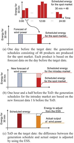
Figure 1 shows the production of generation schedules and adjustment of the actual output by using the ESS. The generation schedules for the spot market are produced, as shown in Figure 1(a). The generation schedules contain 48 products, and each product are based on the forecast data on the day before the target date. The generation schedules for the intraday market are produced, as shown in Figure 1(b). The generation schedules are based on the new forecast data 1.5 h before the ToD to modify the previous generation schedules, because the new forecast data are likely to contain less errors than the previous forecast data on the target day. As shown in Figure 1(c), the difference between the generation schedule and actual output is charged to or discharged from the ESS at the ToD to satisfy the generation schedule. The ESS cannot discharge or charge when the SOC reaches 0 or 1. In this situation, the total energy obtained after the partial adjustment using the ESS will not satisfy the generation schedules, thereby resulting in imbalance. Moreover, when the difference between the generation schedule and actual output exceeds the rated power of the ESS, the imbalance will also occur.

Figure 1. Production of generation schedules and adjustment of the actual output by using the ESS.

(a) One day before the target date: the generation schedules consisting of 48 products are produced for the spot market. Each product is based on the forecast data on the day before the target date. (b) One hour and a half before the ToD: the generation schedules for the intraday market are based on the new forecast data 1 h before the ToD. (c) ToD on the target date: the difference between the generation schedule and actual output is adjusted by using the ESS.

In this study, four methods are developed to produce the generation schedules. Table 2 lists the scheduling methods. The basic method does not consider the SOC transition and forecast errors. Method 1 considers only the SOC transition. Methods 2 and 3 consider the SOC transition and forecast errors. Method 2 uses a linear regression model to estimate the forecast errors. Method 3 adopts a bagged trees model, which is a machine learning method, to adjust the forecast data. Details are explained as follows.

Table 2. Proposed scheduling methods.

	SOC transition	Forecast errors
Basic method	Not considered	Not considered
Method 1	Considered	Not considered
Method 2	Considered	Considered (Linear regression)
Method 3	Considered	Considered (Bagged trees)

2.1 Basic method

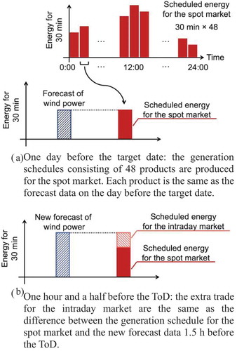
Figure 2 presents an outline of the basic method. In this method, the generation schedules for the spot and intraday markets are the same as the forecast data, that is, the SOC is not considered.

Figure 2. Outline of the basic method.

(a) One day before the target date: the generation schedules consisting of 48 products are produced for the spot market. Each product is the same as the forecast data on the day before the target date. (b) One hour and a half before the ToD: the extra trade for the intraday market are the same as the difference between the generation schedule for the spot market and the new forecast data 1.5 h before the ToD.

2.2 Method 1

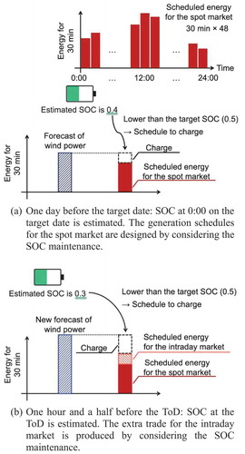
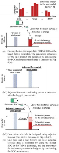
Figure 3 displays an outline of Method 1. The generation schedules for the spot and intraday markets are produced by considering the SOC transition. As shown in Figure 3(a), the SOC at 0:00 on the target date is estimated 1 day before the target date. The estimated SOC is compared with the target SOC, which is 0.5 in this study, and the amount of electricity required to charge or discharge is calculated. Then, the generation schedules for 48 products in the spot market are produced to distribute the calculated electricity with linearly decreasing and maintain the appropriate SOC. Moreover, the SOC at the ToD is estimated 1.5 h before the ToD, and the difference between the estimated and target SOCs is calculated, as shown in Figure 3(b). The SOC maintenance is required to minimize the imbalance. Therefore, the extra trade of purchase or sale for the intraday market is determined to assign the estimated electricity requirement. This method has been reported at conferences [10,11].

Figure 3. Outline of method 1.

(a) One day before the target date: SOC at 0:00 on the target date is estimated. The generation schedules for the spot market are designed by considering the SOC maintenance. (b) One hour and a half before the ToD: SOC at the ToD is estimated. The extra trade for the intraday market is produced by considering the SOC maintenance.

2.3 Method 2

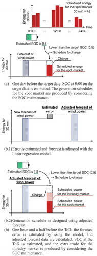
Figure 4 exhibits an outline of Method 2. As shown in Figure 4(a), the generation schedules for the spot market are produced by considering the SOC transition similar to Method 1. However, the generation schedules for the intraday market are produced by considering not only the SOC transition but also the forecast errors. As presented in Figure 4(b.1), the forecast errors are estimated 1.5 h before the ToD, and the adjusted forecast data are calculated by combining the estimated errors and original forecast data. Then, generation schedules that consider the SOC transition are produced on the basis of the adjusted forecast data, as shown in Figure 4(b.2). This step is the same as Method 1.

Figure 4. Outline of method 2.

(a) One day before the target date: SOC at 0:00 on the target date is estimated. The generation schedules for the spot market are produced by considering the SOC maintenance. (b.1) Error is estimated and forecast is adjusted with the linear regression model. (b.2) Generation schedule is designed using adjusted forecast. (b) One hour and a half before the ToD: the forecast error is estimated by using the model, and adjusted forecast data are calculated. SOC at the ToD is estimated, and the extra trade for the intraday market is produced by considering the SOC maintenance.

The models for estimating forecast errors are based on linear regression. The linear regression used in this study is the common and simple model for expressing the relationship between a predictor variable x and response variable y as a linear equation without an intercept. The model is shown in Equation (1), where a indicates a regression coefficient.

(1) $y=ax.$(1)

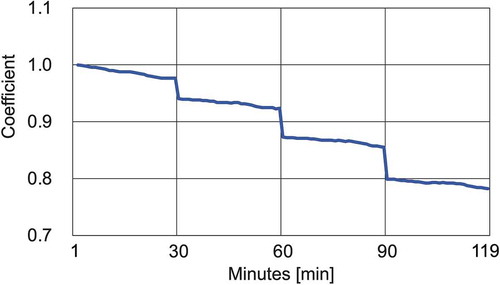
Table 3 presents the modelling condition. The predictor variable is the forecast error at the current time, and the response variable is each forecast error that appears in 1–119 min. Hence, a total of 119 models are produced. Figure 6(a) displays the relationship between the predictor and response variables. The data for learning the model are the same as those for evaluation. The data are from April 2012 to March 2013. These models are produced by using the ‘fitlm’ function of MATLAB 2018a. When the generation schedules are produced, the required forecast errors are calculated by multiplying 119 regression coefficients and the current forecast error. Figure 7 shows the result of coefficients obtained by this model. The coefficient decreases as time passes, and it changes considerably every 30 min. This result is attributed to the time resolution of the forecast data, which is 30 min.

Table 3. Conditions for the linear regression model.

Predictor variable	Forecast errors at the current time
Response variable	Forecast error that appears in 1–119 min
Data for learning the model	Data from April 2012 to March 2013
Data for evaluation	Data from April 2012 to March 2013

2.4 Method 3

Figure 5 exhibits an outline of Method 3. The steps of this method are almost similar to those of Method 2. However, the adjusted forecast data are estimated directly in this method, as shown in Figure 5(b.1). In other words, the adjusted forecast data are not calculated with forecast errors.

Figure 5. Outline of method 3.

(a) One day before the target date: SOC at 0:00 on the target date is estimated. The generation schedules for the spot market are designed by considering the SOC maintenance (this step is the same as Fig. 4(a)). (b.1) Adjusted forecast considering errors is estimated with the bagged trees model. (b.2) Generation schedule is designed using adjusted forecast (this step is the same as Fig. 4(b.2)). (b) One hour and a half before the ToD: adjusted forecast data is estimated by using the model. SOC at the ToD is estimated, and the extra trade for the intraday market is designed by considering the SOC maintenance.

The models for adjusting the forecast data are based on a bagged trees model. The bagged trees model is a machine learning model, which means regression trees using bagging [15].

Table 4 shows the modelling conditions. Four patterns of target timings adjust the forecast data. The predictor variables are the ‘actual output data at the current time,’ ‘forecast data at the current time,’ and ‘forecast data in the target timing.’ At the first target timing, that is, Pattern 1 in Table 4, forecast data in the target timing are the same as those at the current time. The mean value of the actual output data in the ToD is used as the response variable in the learning stage. Figure 6(b) presents the relationship between the predictor the response variables. The predictor and response variables are modified every 30 min. The data for learning the model are the same as those for evaluation. The data are from April 2012 to March 2013. The minimum leaf size and the number of learners are default settings. The ‘Bagged Trees’ application in the Statistics and Machine Learning Toolbox of MATLAB 2018a is used for the models. A fivefold cross-validation is included.

Table 4. Conditions for the bagged trees model.

Patterns of target time	Pattern 1: in 0–30 min Pattern 2: in 30–60 min Pattern 3: in 60–90 min Pattern 4: in 90–120 min
Predictor variable	Actual output at the current time Forecast data at the current time Forecast data in the target timing
Response variable	Adjusted forecast in the target timing
Data for learning the model	Data from April 2012 to March 2013
Data for evaluation	Data from April 2012 to March 2013
Cross-validation folds	5 folds
Minimum leaf size	8
Number of learners	30

Figure 6. Relationship between the predictor and response variables on each model.

(a) Linear regression model. (b) Bagged trees model.

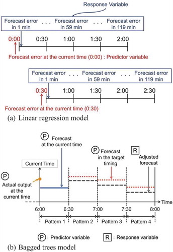
Figure 7. Coefficient obtained by the linear regression model.

3. Simulation and conditions

3.1 Data to use

The forecast data and actual output data of the wind farms in the Tohoku region in Japan are used in this study. The total rated output of wind farms is 442.3 MW. The term of these data is 1 year (from April 2012 to March 2013). The time resolutions of the forecast data and actual output data are 30 and 1 min, respectively. The forecast data are generated by a forecast system explained by Aoki et al. [16]. The forecast data for the spot market are generated at 6:00 on each day, and the forecast horizon is 24 h (0:00–24:00). The forecast data for the intraday market are generated at 0:00, 6:00, 12:00, and 18:00, and each forecast horizon is 24 h. In this study, 1 pu is defined as 442.3 MW, which is the same as the total rated output of wind farms.

3.2 ESS conditions

Five patterns of power are considered for one pattern of hours to discharge. The charge or discharge efficiency depends on the ratio of the required power to the power capacity. When the ratio is lower than 0.5, the efficiency varies linearly from 0.9 to 0.95. By contrast, the efficiency is 0.95 when the ratio exceeds 0.5. The target SOC is fixed as 0.5 for all scheduling methods. Table 5 presents the conditions.

Table 5. Condition of the ESS.

Power [pu]	0.1, 0.2, 0.3, 0.4, 0.5
Hours to discharge [h]	3
Charge/discharge efficiency	Ratio is lower than 0.5: varies linearly from 0.9 to 0.95 Ratio exceeds 0.5: 0.95
Target SOC	0.5

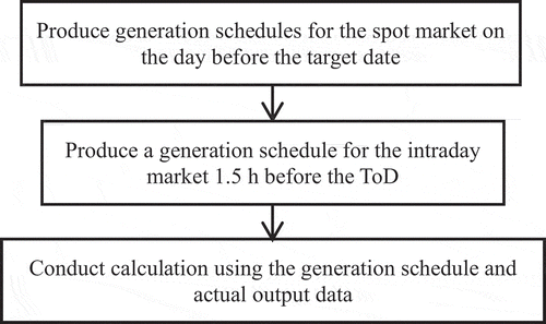
3.3 Simulation outline

Figure 8 shows the simulation outline. The generation schedules, including 48 products for the spot market, are produced initially. Then, the generation schedule for the intraday market is created. Subsequently, calculation with the ESS is conducted to correspond the actual output data to the generation schedule data.

Figure 8. Simulation outline.

3.4 Calculation steps

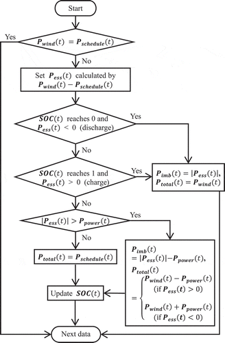
Figure 9 displays the calculation flow in the ToD. The actual wind output data $P_{wind}\left(t\right)$ are compared with the generation schedule $P_{schedule}\left(t\right)$. Their difference is adjusted by $P_{ess}\left(t\right)$, which is the amount of energy for charging to or discharging from the ESS. $P_{ess}\left(t\right)$ cannot be discharged when the $SOC\left(t\right)$ reaches 0. Moreover, $P_{ess}\left(t\right)$ cannot be charged when the $SOC\left(t\right)$ reaches 1. In these cases, the generation schedule is not satisfied. Thus, actual output $P_{wind}\left(t\right)$ is supplied to a power system as $P_{total}\left(t\right)$, and the imbalance $P_{imb}\left(t\right)$ is calculated as the absolute value of $P_{ess}\left(t\right)$. When $P_{ess}\left(t\right)$ exceeds the rated power of the ESS $P_{power}\left(t\right)$, $P_{power}\left(t\right)$ is charged or discharged instead of $P_{ess}\left(t\right)$. At this time, $P_{imb}\left(t\right)$ is calculated by the absolute value of $P_{ess}\left(t\right)$ minus $P_{power}\left(t\right)$, and $P_{total}\left(t\right)$ is computed as $P_{wind}\left(t\right)$ minus $P_{power}\left(t\right)$ if $P_{ess}\left(t\right)$ exceeds 0. Conversely, $P_{total}\left(t\right)$ is calculated as $P_{wind}\left(t\right)$ plus $P_{power}\left(t\right)$ if $P_{ess}\left(t\right)$ does not exceed 0. Furthermore, $SOC\left(t\right)$ is updated in accordance with $P_{power}\left(t\right)$. In all other cases, the generation schedule is satisfied, and $P_{total}\left(t\right)$ equals to $P_{schedule}\left(t\right)$. $SOC\left(t\right)$ is updated in accordance with $P_{ess}\left(t\right)$. The calculation is performed with the next data after these processes. Finally, annual values of $P_{imb}\left(t\right)$ are calculated and evaluated.

Figure 9. Flow of the calculation in ToD (30 min).

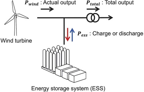
Figure 10 shows the assumed system consisting of wind turbines and the ESS.

Figure 10. Assumed system consisting of wind turbines and the ESS.

4. Results

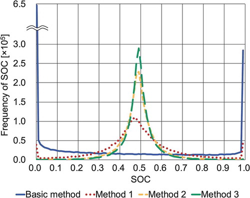
4.1 SOC frequency

Figure 11 illustrates the SOC histogram in each method. This histogram indicates the frequency of SOC every 1 min in a year. As shown in Figure 11, the SOC in Method 3 stayed at approximately 0.5 longer than that in other methods. Thus, the ESS is used most efficiently by Method 3.

Figure 11. Histogram of SOC.

4.2 Results of trades

Table 6 presents the results of trades when a rated power of the ESS was 0.1 pu. The bid volume means the amount of electricity up for bids. Annual generated energy was 2296.6 pu-h. In comparison with the basic method, three proposed methods required more bid values to maintain the SOC in the intraday market. However, the ratio of the imbalance to total bid values in Method 3 was the least.

Table 6. Results of trades.

		Basic Method	Method 1	Method 2	Method 3
Spot market	Bid volume (sale) [pu-h]	2290.6	2286.3	2287.1	2287.3
Intraday market	Bid volume (sale) [pu-h]	247.5	325.9	391.4	374.2
	Bid volume (purchase) [pu-h]	−238.1	−342.4	−408.9	−389.4
Total bid volume [pu-h]		2300.0	2269.8	2269.5	2272.1
Imbalance [pu-h]		291.6	140.9	80.1	47.4
The ratio of the imbalance to total bid volume [%]		12.7	6.2	3.5	2.1

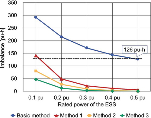
4.3 Imbalance

Figure 12 shows the imbalance between supplied energy and the generation schedules on each method. Figure 12 indicates that the degree of the imbalance in Method 3 is the least. Moreover, the minimum imbalance in the basic method was 126 pu-h. The basic method required a rated power of 0.5 pu when the imbalance of 126 pu-h was allowed. By contrast, Method 1 required a rated power of 0.2 pu to fulfill the condition that the imbalance was 126 pu-h. Methods 2 and 3 required a rated power of 0.1 pu. Therefore, in comparison with the basic method, Methods 2 and 3 could reduce 80% of the rated power when the allowed imbalance was 126 pu-h.

Figure 12. Imbalance between supplied energy and the generation schedules.

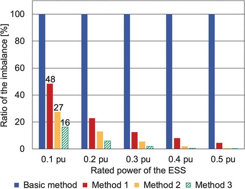
Figure 13 presents the ratio of the imbalance on each proposed method to that in the basic method. As shown in Figure 13, the reduction rate was 84% when Method 3 was used instead of the basic method and the rated power of the ESS was the minimum (0.1 pu). These results indicate that Method 3 is the most successful method for producing generation schedules.

Figure 13. Ratio of the imbalance in each proposed method to that in the basic method.

5. Conclusion

In this paper, three scheduling methods for wind farms for the spot and intraday markets were proposed. A wind farm consisting of wind turbines and the ESS was assumed, and its generation schedules were produced on the basis of forecast data. Method 1 considered only the SOC transition, whereas Methods 2 and 3 considered the SOC transition and forecast errors to maintain the appropriate SOC and minimize the imbalance. Method 2 used the linear regression model to estimate the forecast errors. Method 3 adopted the bagged trees model, which is a machine learning method, to adjust forecast data. On the basis of comparison results among the three proposed methods and the basic method, whose generation schedules are equal to the forecast, Method 3 most efficiently used the ESS. Furthermore, Method 3 could reduce 84% of the imbalance from the generation schedules, even when the rated power of the ESS was the minimum, such as 0.1 pu. Moreover, Methods 2 and 3 could reduce 80% of the rated power when the allowed imbalance was 126 pu-h.

This study revealed the importance of considering the SOC transition and forecast errors for generation scheduling. Results indicated that the proposed methods help produce further correct and practical generation schedules. In future works, we plan to divide the learning data to estimate forecast errors from the data for generation scheduling.

Acknowledgments

This paper is based on results obtained from a project commissioned by the NEDO.

Disclosure statement

No potential conflict of interest was reported by the authors.

Additional information

Funding

This work was supported by the New Energy and Industrial Technology Development Organization [-].

Notes on contributors

Aki Kikuchi

Aki Kikuchi received a Bachelor of Engineering degree in electrical engineering and bioscience from Waseda University, Japan, 2018. She is a graduate student of the Department of Electrical Engineering and Bioscience in Waseda University, Japan. Her research interests include scheduling methods of wind power generation with an ESS in the electricity market. She is a student member of the Institute of Electrical Engineering of Japan.

Masakazu Ito

Masakazu Ito is an associate professor at the Advanced Collaborative Research Organization for Smart Society in Waseda University, Japan. He is studying smart grid technologies, especially those with PV systems and energy storages. He earned his Ph.D. from the Tokyo University of Agriculture and Technology. He started as an assistant professor in the Tokyo Institute of Technology. He then became a JSPS research fellow at the CEA at INES in France, researching life-cycle analysis and remote sensing for large-scale photovoltaic systems.

Yasuhiro Hayashi

Yasuhiro Hayashi (M ’91) received his B. Eng., M. Eng., and D. Eng. degrees from Waseda University, Japan, in 1989, 1991, and 1994, respectively. In 1994, he became a research associate at Ibaraki University, Mito, Japan. In 2000, he became an associate professor in the Department of Electrical and Electronics Engineering, Fukui University, Fukui, Japan. He has been with Waseda University as a professor of the Department of Electrical Engineering and Bioscience since 2009 and as a director of the Research Institute of Advanced Network Technology since 2010. Since 2014, he has been a dean of the Advanced Collaborative Research Organization for Smart Society at Waseda University. His current research interests include the optimization of distribution system operation and forecasting, operation, planning, and control concerned with renewable energy sources and demand response. He is a member of the Institute of Electrical Engineers of Japan and a regular member of CIGRE SC C6 (Distribution Systems and Dispersed Generation).

References

- Ito Y. A brief history of measures to support renewable energy: implications for Japan’s FIT review obtained from domestic and foreign cases of support measures. IEEJ. 2015 Oct. https://eneken.ieej.or.jp/data/6330.pdf
- Guerrero-Mestre V, de la Nieta AAS, Contreras J, et al. Optimal bidding of a group of wind farms in day-ahead markets through an external agent. IEEE Trans Power Syst. 2016 Jul;31(4):2688–2700.
- Tang Y, Ling J, Ma T, et al. A game theoretical approach based bidding strategy optimization for power producers in power markets with renewable electricity. Energies. 2017 May;10(5):627.
- Gomes ILR, Pousinho HMI, Melício R, et al. Optimal wind bidding strategies in day-ahead markets. Technol Innovation Cyber-Phys Syst. 2016;470:475–484.
- Dicorato M, Forte G, Pisani M, et al. Planning and operating combined wind-storage system in electricity market. IEEE Trans Sustainable Energy. 2012 Apr;3(2):209–217.
- Fabbri A, Román TGS, Abbad JR, et al. Assessment of the cost associated with wind generation prediction errors in a liberalized electricity market. IEEE Trans Power Syst. 2005 Aug;20(3):1440–1446.
- Anupam AT, Viassolo DE, Xie L. Robust bidding strategy for wind power plants and energy storage in electricity markets. Proceedings of General Meeting of the IEEE-Power-and-Energy-Society; 2012 Jul; San Diego, CA.
- Ding H, Hu Z, Song Y. Rolling optimization of wind farm and energy storage system in electricity markets. IEEE Trans Power Syst. 2015 Sep;30(5):2676–2684.
- Cai Z, Bussar C, Stöcker P, et al. Optimal dispatch scheduling of a wind-battery-system in german power market. Energy Procedia. 2016;99:137–146.
- Kikuchi A, Ito M, Hayashi Y. Comparative study on state of charge controls of an energy storage system for day-ahead wind-power generation planning. IEEJ Power and Energy Conference; 2017 Sep; Tokyo, Japan. (in Japanese)
- Kikuchi A, Ito M, Hayashi Y. Scheduling methods of wind power generation considering state-of-charge transition for the intraday market. The 2018 Annual Meeting of the Institute of Electrical Engineers of Japan; 2018 Mar; Fukuoka, Japan. (in Japanese)
- Takayama S, Ishigame A. Fluctuation suppression control of wind power generation utilizing deterministic optimization method. 2nd IEEE Annual Southern Power Electronics Conference (SPEC); 2016 Dec; Auckland, New Zealand.
- Yoshida K, Negishi S, Takayama S, et al. A scheduling operation method of wind farm to deal with ramp events and evaluation of required battery capacity. IEEJ Trans Power Energy. 2017;137(10):687–696. (in Japanese).
- Hamamoto A, Hara R, Kita H. Study on suppression of wind farms outputs fluctuation by a HP/BG heat supply system. IEEJ Trans Power Energy. 2017;137(6):446–452. (in Japanese).
- Breiman L. Bagging predictors. Mach Learn. 1996;24:123–140.
- Aoki I, Tanikawa R, Hayasaki N, et al. Development and operational status of wind power forecasting system. IEEJ Trans Power Energy. 2013;133(4):366–372. (in Japanese).