Comparison of support vector machine, random forest and neural network classifiers for tree species classification on airborne hyperspectral APEX images

ABSTRACT

Knowledge of tree species composition in a forest is an important topic in forest management. Accurate tree species maps allow for much more detailed and in-depth analysis of biophysical forest variables. The paper presents a comparison of three classification algorithms: support vector machines (SVM), random forest (RF) and artificial neural networks (ANN) for tree species classification using airborne hyperspectral data from the Airborne Prism EXperiment sensor. The aim of this paper is to evaluate the three nonparametric classification algorithms (SVM, RF and ANN) in an attempt to classify the five most common tree species of the Szklarska Poręba area: spruce (Picea alba L. Karst), larch (Larix decidua Mill.), alder (Alnus Mill), beech (Fagus sylvatica L.) and birch (Betula pendula Roth). To avoid human introduced biases a 0.632 bootstrap procedure was used during evaluation of each compared classifier. Of all compared classification results, ANN achieved the highest median overall classification accuracy (77%) followed by SVM with 68% and RF with 62%. Analysis of the stability of results concluded that RF and SVM had the lowest variance of overall accuracy and kappa coefficient (12 percentage points) while ANN had 15 percentage points variance in results.

KEYWORDS:

• Support vector machines
• random forest
• artificial neural networks
• hyperspectral data
• classification

View correction statement:

Corrigendum

Introduction

Knowledge about the vegetation condition of a forested area is important both for monitoring of protected areas (Nagendra et al., 2013) and estimating the potential economic value of forests (Ashutosh, 2012). Integrated management requires accurate and multifaceted mastery of forest information, of which the forest ecosystem cover is the most basic and important component (Shen, Sakai, Hoshino, 2010). One of the regions that has been endangered by human activities is the Karkonosze Mountains. A section of the Karkonosze National Park forms part of the valuable Karkonosze Mountains ecosystem. More than 30 years ago, a rapid expansion of industry in the surrounding areas combined with the particular landscape of Karkonosze to cause acid rains that exposed the fragile mountain ecosystem to insect infestation (Jadczyk, 2009). The synergic effect of acid rains, air pollution, drought and insect outbreak which all happened at that time contributed to the severity of the damage done to the ecosystem. It is also worth mentioning that spruces planted in the Karkonosze before 1980 were not typical of a mountain ecosystem and had lower resistance to the rough mountain climate. Although damage was not as severe as some predicted, it is the evidence of unreasonable decisions and a lack of planning and foresight in treating areas of special value (Raj, 2014). Hence, detailed information about vegetation recovery is crucial for the national park administration and foresters alike. Only low-scale Landsat-based analyses describing general information on the state of vegetation before the disaster are available (Bochenek, Ciołkosz, & Iracka, 1997; Jarocińska et al., 2014). With the use of advanced hyperspectral sensors such as Airborne Prism Experiment (APEX), a deeper analysis of vegetation can be made (Jarocińska et al., 2016; Peerbhay, Mutanga, & Ismail, 2013). The large amount of information contained in hyperspectral data allows for much more accurate and detailed classifications of tree species and vegetation (Masaitis & Mozgeris, 2013; Thenkabail, Lyon, & Huete, 2012). Furthermore, more traditional ways of classifying tree species demand a lot of manpower and money (Peerbhay et al., 2013).

One of the first papers addressing forest species classifications using hyperspectral data was the research conducted by the U.S. Geological Survey in 2003 (Kokaly, Despain, Clark, & Livo, 2003). The authors identified eight classes of forest cover using an expert system and Airborne Visible–Infrared Imaging Spectrometer data. Among classified tree species were spruce, lodgepole and whitebark pine, aspen and Douglas fir. The researchers obtained an overall accuracy of 74.1%, and kappa coefficient of 0.62. Another study by a group of researchers (Shen et al., 2010) concluded that the best tree species classification results were achieved using spectral angle mapper, followed closely by support vector machine (Shen et al., 2010). Another research used Digital Airborne Imaging Spectrometer (DAIS 7915) hyperspectral data to map 42 different communities and land cover types of the High Tatra Mountains. It was proven that high spectral resolution data can be effectively used to map diverse mountain tree and non-tree vegetation with a high degree of accuracy (Marcinkowska et al., 2014; Zagajewski, 2010). Successful tree species mapping using airborne imaging spectrometer for applications (AISA) hyperspectral data was conducted by Peerbhay et al. The authors used the near infrared (NIR) spectral range for classification of six exotic tree species, achieving 88% overall accuracy with a kappa coefficient of 0.87 (Peerbhay et al., 2013). Most forest researchers focus on the NIR spectral range for forest-related analysis because most features typical to green vegetation can be found in this region (red edge, chlorophyll and other pigment absorption bands). Some studies show that adding shortwave infrared data from the spectral range between 1000 and 2500 nm can improve tree species classification accuracy (Lucas, Bunting, Paterson, & Chisholm, 2008).

The random forest (RF) algorithm has been successfully used in the past, providing accurate land cover maps (Ghimire, Rogan, & Miller, 2010; Pal, 2005). Studies using hyperspectral data for forest sciences showed that RF can be successfully used to detect insect infestations, extract physiological plant characteristics (Doktor, Lausch, Spengler, & Thurner, 2014), estimate plant biomass (Elhadi, Onisimo, Abdel-Rahman, & Riyad, 2014) or map plant species (Burai, Deak, Valko, & Tomor, 2015). The study by Naidoo et al. showed the potential for using lidar and hyperspectral data with RF modeling. The hybrid approach proposed by the authors proved an overall accuracy of 87%, which was significantly higher than the model using only spectral data (80%) (Naidoo, Cho, Mathieu, & Asner, 2012).

SVM is often claimed to be the best at dealing with complex classification problems such as tree species differentiation, followed by RF (Ghosh, Fassnacht, Joshi, & Koch, 2014; Suess et al., 2015). The study by Ghosh et al. using information in a broader electromagnetic spectrum (450–2500 nm) focused on classifying five tree species in managed forests of central Germany using SVM and RF on Hyperion and HyMap data. Using only spectral information, the overall classification accuracies on a 4-m pixel hyperspectral image was 71% for SVM and 72% for RF. Both classifiers showed similar results for this scale (Ghosh et al., 2014).

Artificial neural networks (ANNs) are a commonly used tool in remote sensing of the Earth’s surface that often achieves the same accuracies as RF and SVM (Petropoulos, Kontoes, & Keramitsoglou, 2012). They have been successfully applied to estimation of biophysical forest parameters for multispectral data (Linderman et al., 2004), biomass and soil moisture retrieval (Ali, Greifeneder, Stamenkovic, Neumann, & Notarnicola, 2015), crop monitoring (Gupta et al., 2015) or land cover classification (Petropoulos et al., 2012). Despite all those uses for ANN, the topic of tree species classification using ANN is seldom approached by the research community. The paper by Omer et al. used a multilayered feed-forward ANN to map tree species on WorldView-2 (WV-2) data, achieving results comparable to those obtained from other classification algorithms (Omer, Mutanga, Abdel-Rahman, & Adam, 2015; Priedītis et al., 2015). A systematic search of the literature revealed that in recent years there has been a high number of studies on the use of ANN in remote sensing (Fassnacht et al., 2016; Mas & Flores, 2008), but there is a severe lack of research in tree species classification using ANNs and hyperspectral data, as compared to other methods.

The aim of this paper is to evaluate three nonparametric classification algorithms (SVM, RF and ANN) in an attempt to classify the five most common tree species of the Szklarska Poręba area: spruce (Picea alba L. Karst), larch (Larix decidua Mill), alder (Alnus Mill), beech (Fagus sylvatica L.) and birch (Betula pendula Roth).

Research area

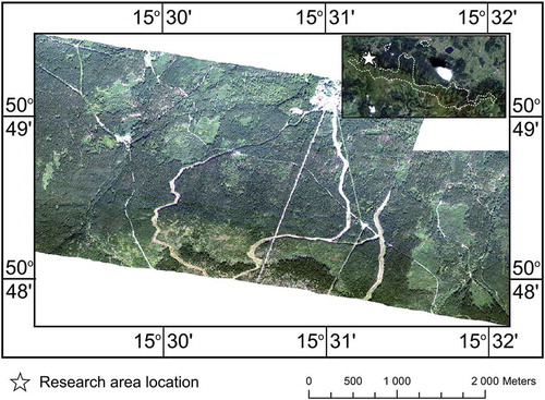
The research area is located in the northwestern part of the Karkonosze National Park, Poland, south of Szklarska Poręba town. The Karkonosze National Park and its Czech counterpart are located on the Polish–Czech border (Figure 1). The parks cooperate with each other in terms of ecosystem management and protection. This cooperation resulted in the inclusion of both parks in the UNESCO’s Man and Biosphere (M&B) international reserve network. Moreover, both parks are members of the EUROPARC Federation and were awarded Transboundary Park Programme certificate in 2004. The whole area of the Karkonosze National Park is part of the European Natura 2000 biological network. The main land cover type is subalpine forest dominated by spruce, with an admixture of beech and occasional larch and birch stands in lower parts of mountain slopes. The classified scene covers the northern slopes of the Karkonosze Mountains near Szklarska Poręba village.

Figure 1. Research area location.

Data

The classifications were made based on APEX hyperspectral data. APEX is a dispersive push-broom system with a 28-degree field of view developed by a Swiss–Belgian consortium under the framework of the ESA-PRODEX program (Itten et al., 2008). Two spectrometers cover the spectral range of 380–2500 nm (Hueni et al., 2009) (Table 1). APEX data were collected during a campaign of flights in September 2012, from the standard APEX imaging platform – a German Dornier Do 228 aircraft, belonging to DLR (German Aerospace Agency). The collected data were then processed by sensor operator VITO (Flemish Institute for Technological Research), which made atmospheric, radiometric and geometric image corrections. The resultant processed data had 288 spectral bands in the range from 413 to 2447 nm and a 3.35-m spatial resolution.

Table 1. Selected APEX characteristics (based on Popp et al. (2012)).

Characteristic	VNIR	SWIR
Spectral range	380–971.7 nm	941.2–2501.5 nm
Spectral bands	Up to 334	198
Spectral sampling interval	0.6–6.3 nm	6.2–11 nm
Field of view (FOV)	28°
Instantaneous field of view (IFOV)	0.028° (≈0.5 mrad)
Spatial resolution	2.5 m @ 5000 AGL

Methods

The first step in preprocessing of data before classification procedures was to reduce the data dimensionality. This step was aimed at reducing processing times and developing ways to use less of the data but still be able to achieve satisfying results. The 288-band APEX dataset was first reduced to 222 bands by removal of noisy bands from the beginning and end of the spectral range, plus removal of water vapor absorption bands. Bands located in water vapor absorption regions are usually interpolated from data while undergoing atmospheric correction. In the presented dataset, all bands in water vapor absorption ranges were masked with a value of 1.0005 by the data manufacturer and therefore contained no useful data. The next step focused on selecting the best bands from the 222-band dataset. Based on the work by Pal and Mather (2006), a 40-band dataset was deemed to be optimal for processing times while preserving enough data to obtain satisfactory results. Principal component analysis (PCA) was used for band selection. Based on past works (Sommer et al., 2015; Thenkabail et al., 2012), one can assess the importance of each spectral band in each principal component by taking a look at the magnitude of factor loadings which correspond to the correlations between bands and principal components. This step assigns each spectral band a loading that indicates its importance. Higher loadings indicate more important bands. This procedure allowed us to select the 40 spectral bands with the highest PCA loadings from our 222-band dataset. The selected bands were then used for classification purposes.

Training and testing samples were obtained during the field research conducted in 2013 and 2014. During data collection, localization of selected tree species was obtained. During field data collection, only areas currently occupied by living trees more than 5 m tall were considered as valid location sources. The selected sampling sites had to be occupied by trees of the same species with a minimum of five trees in a 4-m radius from the GPS receiver. It was decided to only use measurements with a localization error below 2 m. This allowed for collection of nine pixels in a 3 × 3 window centered on the GPS location measurement. For larger areas, the locations of polygon corners were collected and then used for pixel extraction. Areas clearly in shadow and ambiguous pixels were excluded. Then these locations were used to extract training and testing samples from the 40-band APEX dataset. Some classifiers, such as RF, are easily biased by an odd number of samples in classes (Breiman, 2001). To ensure that odd sample numbers do not cause biases which might influence results, every classified species is represented by 120 pixels.

Most supervised classifiers are sensitive to data used for training, hence classification results will also change depending on the training dataset. Furthermore, to remove bias introduced by humans into classification results, we decided to follow a procedure involving random selection of training and testing datasets. Based on the work by Braga-Neto and Dougherty (2014)and Ghosh et al. (2014), we decided to use the 0.632 bootstrap approach for generating the test and training dataset. The whole procedure was divided into a number of separate iterations. Each iteration involves random splitting of all samples into test and training dataset so that 63.2% of all samples are assigned to the training dataset and the remaining serve as the test dataset, which is excluded from the classifier training process. The exact number of samples/pixels representing each class can be seen in Table 2. After this step, classification was made using the selected training samples and the chosen classification algorithm. The resulting classification result went through an accuracy assessment procedure in which overall accuracy, kappa coefficient, and producer and user accuracies were calculated for classes. The number of iterations for each classifier was set to 100. Data collected during iterations were used to compare SVM, RF and ANN classifiers and to draw boxplots of user and producer accuracies for classes and boxplots of overall accuracy and kappa coefficient for each used classification algorithm. Every classification algorithm used the same training data and was tested on the same test data as every other, in order to guarantee comparability between results.

Table 2. Training and testing sample sizes (in pixels) used for classifications.

	Birch	Beech	Larch	Alder	Spruce
Training sample	76	76	76	76	76
Testing sample	44	44	44	44	44

We compared three supervised nonparametric classification algorithms: SVM, RF and ANN in this paper. Processing of data and classifications were conducted using R statistical software (R Core Team, 2015).

The SVM classification algorithm is commonly employed in remote sensing in a range of applications (Marcinkowska et al., 2014; Pal & Mather, 2006; Rajee, Hitendra, & Kushwaha, 2014). The SVM algorithm was developed by Vapnik (1995). The SVM classifier tries to find the optimal hyperplane in n-dimensional classification space with the highest margin between classes. SVM is often reported to achieve better results than other classifiers (Ghosh et al., 2014; Huang, Davis, & Townshed, 2002; Sluiter & Pebesma, 2010). SVM classification was conducted using the “e1071” package (Meyer, Dimitriadou, Hornik, Weingessel, & Leisch, 2015). Because of the relative complexity of our problem, we decided to select the radial kernel, with gamma and cost parameters being selected by tune.svm procedure for gamma values from 0.1 to 1 with a step of 0.1 and cost values from 0 to 128 with a step of 8. The tune.svm procedure runs a 10-fold cross validation on a dataset to provide the best combination of cost and gamma parameters.

The RF classifier was developed by Breiman (2001) and can be described as an ensemble of classification trees, where each tree votes on the class assigned to a given sample, with the most frequent answer winning the vote (Sun & Schulz, 2015). The RF algorithm has proven to handle high dimensional data well and is relatively resistant to overfitting (Breiman, 2001). RF classification was done using the “randomForest” package (Liaw & Wiener, 2002). There are two parameters that have to be chosen before model training: the number of predictors taken into consideration at each fork of the tree (mtry) and the number of random trees assembled during model building (ntree). Before the classification step, the RF model was tuned. In effect, an mtry value of 24 was chosen as optimal for the presented dataset. Previous research strongly implies that ntree values have a low impact on final results, and we therefore decided to use 500 random trees to create the final model (Breiman & Cutler, 2004).

An ANN classifier can be described as a parallel computing system consisting of an extremely large number of simple processors with interconnections (Huang et al., 2002, following Jain, Duin, & Mao, 2000). One commonly used type of neural network is a multilayered feed-forward perceptron that consists of several layers of neurons connected with each other. The multilayered perceptron can separate data that are nonlinear and generally consists of three or more types of layers (Beluco, Engel, & Beluco, 2015). ANNs have successfully been applied to remote sensing in many fields (Mas & Flores, 2008; Zagajewski, 2010; Zhang & Xie, 2012). ANN classification was done with the help of R statistical software (R Core Team, 2015) and the “nnet” package (Venables & Ripley, 2002). The “nnet” package is capable of simulating feed-forward neural networks with a single hidden layer with a backpropagation algorithm as the training algorithm (Werbos, 1994). For the training step, we used the following parameters: 24 neurons in the hidden layer, a decay value of 0.0005 and a training stop condition of 0.0001.

The last step was to compare classifiers analyzing the variation of producer and user classification accuracies for classes, and the variability of overall accuracy and kappa coefficient. Based on those results, the best (most accurate) iteration for each classification algorithm was selected. The best iteration parameters were then used to produce final classification images. Non-forested areas were masked from final images using a normalized digital surface model and normalized difference vegetation index (NDVI)-based mask. Vegetation smaller than 2.5 m was masked to avoid classification of bushes and young tree stands. To remove buildings and manmade materials, pixels with an NDVI value lower than 0.2 were also masked. The scene used had no cloud coverage.

Results

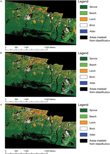
Of all compared classification results, ANN achieved the highest median overall classification accuracy (77%) followed by SVM with 68% and RF with 62%(Figure 2). Similarly for the kappa coefficient, ANN had the highest median kappa, at 0.72, while SVM and RF had 0.61 and 0.52 median kappa, respectively. By changing the training dataset, we were able to provide minimum and maximum accuracies for each classification algorithm, and thus can assess each classifier’s sensitivity to the data used to train it. The lowest variance of overall accuracy and kappa coefficient was achieved by RF and SVM (12 percentage points) while ANN had 15 percentage points. Hence, RF and SVM classifiers are less sensitive to changing datasets than ANN, with a difference of 3 percentage points between them. Analysis of producer and user accuracies shows that some classes are consistently classified with high accuracies while others vary depending of classifier. Of all those classified, the Alder class had the highest median user accuracy (ANN – 94%, SVM – 86%, RF – 78%) and producer accuracy (ANN – 94%, SVM – 82%, RF – 78%) no matter the classification algorithm used. On the other hand, there is no class that is clearly classified worst by all classification algorithms. In the case of ANN and SVM, the class that had the lowest median producer accuracy was birch (ANN – 68%, SVM – 59%) while for RF it was beech (50%). The classes with the lowest median user accuracy were spruce for ANN (69%), larch for RF (50%) and birch for SVM (57%). Apart from analyzing the error measurement parameter, a visual interpretation of results was performed (Figure 2). RF and SVM outputs seem to overestimate the number of pixels classified as larch in upper parts of image, which appears to be mostly covered by spruce forest with some beech stands. Output images also have a slight salt-and-pepper effect which is most noticeable in the lower left part of classification images, and is mostly caused by shadows created by trees in forest.

Figure 2. Classification output images for ANN (a), RF (b) and SVM (c). (Color black symbolizes masked areas – non-forest vegetation and urban areas).

Table 3 and Figure 4 show classified tree species abundances in the research area based on outputs from compared classification algorithms. To calculate these as percentages, the best iteration output for each algorithm was used. No official information regarding real tree species are available for the research area. Only official tree species abundances for the whole park are available, which makes any result comparison to them pointless.

Table 3. Tree species abundances based on SVM, RF and ANN classifications. Values are in percentages.

Class	SVM	Random forest	ANN
Birch	7.77	5.20	4.37
Beech	6.30	6.13	7.13
Larch	19.70	18.09	14.63
Alder	1.75	1.77	0.74
Spruce	64.49	68.80	73.12

Figure 3. Classification results and their user and producer accuracies for ANN ((a) and (b)), RF ((c) and (d)) and SVM ((e) and (f)).

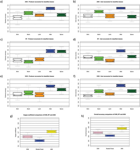
Figure 4. Tree species abundances based on outputs from compared classification algorithms.

Discussion and conclusions

The study concludes that ANN achieved the highest median accuracies among all compared classification algorithms given certain constraints.

The worse accuracies for SVM and RF classifications may be an effect of suboptimal choice of bands used (either their number or the actual bands selected). Using only 40 bands might not be the optimal number of input data for some classification algorithms (SVM, RF) in opposition to the findings of Pal and Mather (2006), but on the other hand it might also be that the wrong 40 bands were selected (not expressing the spectra which provide the best differentiation between classes). The reasons for our decision to limit the number of spectral bands were twofold. First, to allow ANN to work relatively fast, adding more data would lengthen ANN training times to unacceptable levels so that it would be highly impractical to work with them. Larger input datasets will lengthen classification times for ANN more than for SVM and RF. Second, we wanted to provide a generalized dataset of spectral bands that would be useful for classification of tree species based on APEX data. This approach would allow for more robust classification methodologies that provide a more generalized approach to tree species classification. Although a difficult task, such methods would allow for classification methodologies that would be more independent of the spatial and temporal constraints of a given research area. More sophisticated methods of band selection than output spectral bands such as sparse partial least squares-discriminant analysis (PLS-DA), genetic algorithm, SVM-Wrapper, PLS or support vector machine regression were reported to provide better selection of spectral bands than that used in this research (Fassnacht et al., 2014; Feilhauer, Asner, & Martin, 2015), although this holds true to SVM and RF classification algorithms, because ANN were not investigated. It was reported that minimum noise fraction (MNF) transformation outperforms all the aforementioned band selection algorithms (Fassnacht et al., 2014) resulting in higher classification accuracies. The disadvantage of MNF is that it is data dependent, which forces the user to calculate MNF transformed bands for each dataset. Moreover, such MNF datasets can and will be different from each other (both in terms of quality and features present in each MNF band) requiring additional preprocessing before the classification process (Fassnacht et al., 2016).

Second, the number of training and verification pixels for each class might have a bigger impact on SVM and RF than on ANN. Some studies recommended at least 400 pixels per class as the optimal number of pixels for classification purposes (Kavzoglu & Mather, 2003). A small sample size might be not enough for optimal training of SVM and RF, although some studies report high accuracies for RF and SVM using 60 pixels per class (Fassnacht et al., 2014; Ghosh et al., 2014). While dealing with the SVM classifier, it is good to select not only pure pixels but also mixels for your classes, so that the hyperplane calculated by the algorithm has tighter margins separating samples in image space. While having more pixels is always recommended, sometimes it is hard to find a high enough number of pixels representing a given land cover type in a given scene.

The presented 0.632 bootstrap procedure, apart from being useful as an accuracy assessment technique which strengthens belief in classification results, might have other uses. Repeating the classification procedure allows one to observe how accuracy-related parameters (producer, user, overall accuracy and kappa coefficient) change. Such a technique allows for analysis of the distribution of accuracies for classes (showing skewness and variance of accuracy distribution for each class). A high variance in results (for a given class or overall) might indicate that not all training samples present a consistent spectral signature for a classifier to learn. This might be because of samples being taken from areas that are not spectrally pure, samples being a mixture of different land cover types or a given class being spectrally heterogeneous. While useful, it might be tempting to use this procedure to select only pixels that give the highest accuracies. This might be a method for engineering the best pixel sample, disregarding that classification has the objective of delivering results consistent with reality.

ANN have the potential to become a more widely used classification algorithm, but because of their time-consuming parameter tuning procedure, the numerous types of neural network architectures to choose from and the high number of algorithms used for training ANN, some researchers recommend SVM or RF as easier methods which repeatedly achieve results with high accuracies and are often faster (Petropoulos et al., 2012). SVM was widely used for tree species classification purposes (Dalponte, Orka, Gobakken, Gianelle, & Naesset, 2013; Ghiyamat, Shafri, Amouzad, Shariff, & Mansor, 2013; Peerbhay et al., 2013), but there are only a limited number of studies discussing the use of ANN in tree species classification (Omer et al., 2015; Priedītis et al., 2015). The study by Omer et al. applied ANN to map tree species based on multispectral WV-2 data, and achieved a high accuracy (75% and more), but also concluded that SVM is often a tiny bit more accurate (Omer et al., 2015). The other study, by Priedītis et al. (2015), compared linear discriminant analysis (LDA) to ANN using 64 hyperspectral bands in the 400–970 nm spectral range and concluded that ANN performed similarly to LDA. It was also reported that certain tree species were classified with lower accuracies (black alder, European aspen) than others (Scots pine, Norway spruce, silver birch) no matter which classifier was used.

Our findings are in agreement with research by Burai et al. (2015) which reports that SVM classifier outperforms RF (Burai et al., 2015), although some studies report SVM and RF having similar performance (Ghosh et al., 2014).

Field data acquisition can be expensive and difficult because of the difficulty of access to research areas. As such, in our opinion, reference data collection should be done as soon as possible depending on available resources and topic of research. Some studies conduct reference data collection in the same month as hyperspectral data acquisition, helped by available auxiliary resources (maps) (Peerbhay et al., 2013), while others use forest species maps obtained from forest management institutions (public or private) and orthophoto maps (Fassnacht et al., 2014; Ghosh et al., 2014). The aforementioned sources use all available sources not limiting themselves to only one source of information about forest species composition. In this research, the available auxiliary sources were used during the preparatory stage before field data collection. A difference of up to 2 years between data acquisition and reference data collection, as was the case in this paper, did not impact the quality of collected data, since overall forest species composition changes very slowly. Moreover, in protected areas any change can only be introduced by nature or by park staff. Both result in visible changes to surroundings and are easily spotted (stumps, deadwood, logs, etc.).

We recommend more studies be conducted to investigate optimal data selection techniques with a focus on the optimal number of bands used (probably depending on classification algorithm) and optimal selection of spectral bands (which would best express the spectral variability of classes). Also, more work with ANNs and hyperspectral data can be done. It is also worth investigating the use of deep learning artificial networks in hyperspectral remote sensing, although the huge number of bands present in such datasets would require careful selection of data fed into such networks. Third, we recommend further investigation into bootstrapping accuracy assessment techniques such as the 0.632 bootstrap procedure.

ANNs are not commonly used for tree species classification, mainly because it is relatively easier to use SVM or RF. While SVM and RF achieve high accuracies when using MNF transformed bands or a high number of spectral bands, we have showed that by limiting the number of spectral bands used, ANN tend to perform better than SVM or RF. ANNs have a reputation for being hard to use and to optimize, which is true of most implementations which force the user to set all parameters on his own. The software package used for simulation of ANN in this research is relatively easy to use, requires only a limited number of parameters to be set in order to run and is available as open-source software.

Acknowledgments

The authors wish to thank the European Facility for Airborne Research Transnational Access (EUFAR TA) which funded a flight campaign and the Foundation of University of Warsaw for financial support of the field campaign during the HyMountEcos project. Special thanks go to the German Space Agency, for execution of the flight; VITO, for obtaining and processing APEX data; the administration of Karkonosze National Park, for help during field research; and the Institute of Geography and Spatial Organization, Charles University in Prague and the University of Warsaw, who were involved in the whole project.

The research was funded by the Polish Ministry of Sciences and Higher Education from science development funds in 2013–2017 as a research project under the framework of the Diamond Grant Programme.

Field verification of condition analyses were conducted under the Polish–Norwegian Research Programme, National Centre for Research and Development project: Ecosystem stress from the combined effects of winter climate change and air pollution – how do the impacts differ between biomes? (WICLAP), No: POL-NOR/198571/83/2013.

Disclosure statement

No potential conflict of interest was reported by the authors.

Additional information

Funding

The research was funded by the Polish Ministry of Sciences and Higher Education from science development funds in 2013–2017 as a research project under the framework of the Diamond Grant Programme [DI2012020042]. Field verification of condition analyses were conducted under the Polish–Norwegian Research Programme, National Centre for Research and Development project: Ecosystem stress from the combined effects of winter climate change and air pollution – how do the impacts differ between biomes? (WICLAP), No: [POL-NOR/198571/83/2013].

References

- Ali, I., Greifeneder, F., Stamenkovic, J., Neumann, M., & Notarnicola, C. (2015). Review of machine learning approaches for biomass and soil moisture retrievals from remote sensing data. Remote Sensing, 7, 16398–154. doi:10.3390/rs71215841
- Ashutosh, S. (2012). Monitoring forests: A new paradigm of remote sensing & GIS based change detection. Journal of Geographic Information System, 4, 470–478. doi:10.4236/jgis.2012.45051
- Beluco, A., Engel, P.M., & Beluco, A. (2015). Classification of textures in satellite image with Gabor filters and a multilayer perceptron with back propagation algorithm obtaining high accuracy. International Journal of Energy and Environment, 6(5), 437–460. doi:10.5935/2076-2909.20150001
- Bochenek, Z., Ciołkosz, A., & Iracka, M. (1997). deterioration of forests in the Sudety Mountains, Poland, detected on satellite images. Environmental Pollution, 98(3), 375–379. doi:10.1016/S0269-7491(97)00146-2
- Braga-Neto, U.M., & Dougherty, E.R. (2014). Is cross-validation valid for small sample microarray classification? Bioinformatics, 20, 374–380. doi:10.1093/bioinformatics/btg419
- Breiman, L. (2001). Random forests. Machine Learning, 45, 5–32. doi:10.1023/A:1010933404324
- Breiman, L., & Cutler, A. (2004). Random forests. Available at https://www.stat.berkeley.edu/~breiman/RandomForests/cc_home.htm, accessed on 21.04.2016
- Burai, P., Deak, B., Valko, O., & Tomor, T. (2015). Classification of herbaceous vegetation using airborne hyperspectral imagery. Remote Sensing, 7, 2046–2066. doi:10.3390/rs70202046
- R Core Team. (2015). R: A language and environment for statistical computing, R foundation for statistical computing, Vienna, Austria. https://www.R-project.org/.
- Dalponte, M., Orka, H.O., Gobakken, T., Gianelle, D., & Naesset, E. (2013). Tree species classification in boreal forests with hyperspectral data. IEEE Transactions on Geoscience & Remote Sensing, 51(5), 2632–2645. doi:10.1109/TGRS.2012.2216272
- Doktor, D., Lausch, A., Spengler, D., & Thurner, M. (2014). Extraction of plant physiological status from hyperspectral signatures using machine learning methods. Remote Sensing, 6, 12247–12274. doi:10.3390/rs61212247
- Elhadi, A., Onisimo, M., Abdel-Rahman, E., & Riyad, I. (2014). Estimating standing biomass in papyrus (Cyperus papyrus L.) swamp: Exploratory of in situ hyperspectral indices and random forest regression. International Journal of Remote Sensing, 35, 693–714. doi:10.1080/01431161.2013.870676
- Fassnacht, F., Latifi, H., Stereńczak, K., Modzelewska, A., Lefsky, M., Waser, L., … Ghosh, A. (2016). Review of studies on tree species classification from remotely sensed data. Remote Sensing of Environment, 186, 64–87. doi:10.1016/j.rse.2016.08.013
- Fassnacht, F.E., Neuman, C., Forster, M., Buddenbaum, H., Ghosh, A., Clasen, A., … Koch, B. (2014). Comparison of feature reduction algorithms for classifying tree species with hyperspectral data on three central European test sites. IEEE Journal of Selected Topics in Applied Earth Observations and Remote Sensing, 7, 2547–2561. doi:10.1109/JSTARS.2014.2329390
- Feilhauer, H., Asner, G.P., & Martin, R.E. (2015). Multi-method ensemble selection of spectral bands related to leaf biochemistry. Remote Sensing of Environment, 164, 57–65. doi:10.1016/j.rse.2015.03.033
- Ghimire, B., Rogan, J., & Miller, J. (2010). Contextual land-cover classification: Incorporating spatial dependence in land-cover classification models using random forests and the Getis statistic. Remote Sensing Letters, 1, 45–54. doi:10.1080/01431160903252327
- Ghiyamat, A., Shafri, H., Amouzad, M.G., Shariff, A., & Mansor, S. (2013). Hyperspectral discrimination of tree species with different classifications using single- and multiple-endmember. International Journal of Applied Earth Observations and Geoinformation, 23, 177–191. doi:10.1016/j.jag.2013.01.004
- Ghosh, A., Fassnacht, F.E., Joshi, P.K., & Koch, B. (2014). A framework for mapping tree species combining hyperspectral and LiDAR data: Role of selected classifiers and sensor across three spatial scales. International Journal of Applied Erath Observation and Geoinformation, 26, 49–63. doi:10.1016/j.jag.2013.05.017
- Gupta, D.K., Kumar, P., Mishra, V.N., Prasad, R., Dikshit, P.K.S., Dwivedi, S.B., … Srivastava, V. (2015). Bistatic measurements for the estimation of rice crop variables using artificial neural network. Advances in Space Research, 55(6), 1613–1623. doi:10.1016/j.asr.2015.01.003
- Huang, C., Davis, L.S., & Townshed, J.R.G. (2002). An assessment of support vector machines for land cover classification. International Journal of Remote Sensing, 23, 725–749. doi:10.1080/01431160110040323
- Hueni, A., Biesemans, J., Meuleman, K., Dell’Endice, F., Schlapfer, D., Odermatt, D., & Kneubuehler, M. (2009). Structure, components, and interfaces of the Airborne Prism Experiment (APEX) processing and archiving facility. IEEE Transactions on Geoscience and Remote Sensing, 47, 29–43. doi:10.1109/TGRS.2008.2005828
- Itten, K.I., Dell’Endice, F., Hueni, A., Kneubuhler, M., Schlapfer, D., Odermatt, D., & Seidel, F. (2008). APEX – The hyperspectral ESA Airborne Prism Experiment. Sensors, 8, 6235–6259. doi:10.3390/s8106235
- Jadczyk, P. (2009). Natural effects of large-area forest decline in the Western Sudeten. Environment Protection Engineering, 35, 49–56. http://epe.pwr.wroc.pl/2009/Jadczyk_1-2009.pdf
- Jain, A.K., Duin, R.P.W., & Mao, J. (2000). Statistical pattern recognition: A review. IEEE Transactions Pattern Analysis and Machine Intelligence, 22, 4–37. doi:10.1109/34.824819
- Jarocińska, A., Zagajewski, B., Ochtyra, A., Marcinkowska-Ochtyra, A., Kycko, M., & Pabjanek, P. (2014). Process of ecological disaster in Karkonosze and Izerskie Mts. on Landsat satellite images [in Polish: Przebieg klęski ekologicznej w Karkonoszach i Górach Izerskich na podstawie analizy zdjęć satelitarnych Landsat]. In R. Knapik (ed.), Konferencja Naukowa z okazji 55-lecia Karkonoskiego Parku Narodowego: 25 lat po klęsce ekologicznej w Karkonoszach i Górach Izerskich – obawy a rzeczywistość (pp. 47–62). Karpacz: Karkonoski National Park. 16-18.01. 2014. ISBN 978-83-64528-58-3.
- Jarocińska, A.M., Kacprzyk, M., Marcinkowska-Ochtyra, A., Ochtyra, A., Zagajewski, B., & Meuleman, K. (2016). The application of APEX images in the assessment of the state of non-forest vegetation in the Karkonosze Mountains. Miscellanea Geographica – Regional Studies On Development, 20(1), 21–27. , doi:10.1515/mgrsd-2016-0009
- Kavzoglu, T., & Mather, P.M. (2003). The use of backpropagating artificial neural networks in land cover classification. International Journal of Remote Sensing, 24(23), 4097–4938. doi:10.1080/0143116031000114851
- Kokaly, R.F., Despain, D.G., Clark, R.N., & Livo, K.E. (2003). Mapping vegetation in Yellowstone National Park using spectral feature analysis of AVIRIS data. Remote Sensing of Environment, 84, 437–456. doi:10.1016/S0034-4257(02)00133-5
- Liaw, A., & Wiener, M. (2002). Classification and regression by randomForest. R News, 2(3), 18–22.
- Linderman, M., Liu, J., Qi, J., An, L., Ouyang, Z., Yang, J., & Tan, Y. (2004). Using artificial neural networks to map the spatial distribution of understorey bamboo from remote sensing data. International Journal Remote Sensing, 25(9), 1685–1700. doi:10.1080/01431160310001598971
- Lucas, R., Bunting, P., Paterson, M., & Chisholm, L. (2008). Classification of Australian forest communities using aerial photography, CASI and HyMap data. Remote Sensing of Environment, 112(5), 2088–2103. doi:10.1016/j.rse.2007.10.011
- Marcinkowska, A., Zagajewski, B., Ochtyra, A., Jarocińska, A., Raczko, E., Kupkova, L., … Meuleman, K. (2014). Mapping vegetation communities of the Karkonosze National Park using APEX hyperspectral data and support vector machines. Miscellanea Geographica, 18(2), 1–7. doi:10.2478/mgrsd-2014-0007,
- Mas, J.F., & Flores, J.J. (2008). The application of artificial neural networks to the analysis of remotely sensed data. International Journal of Remote Sensing, 29(3), 617–663. doi:10.1080/01431160701352154
- Masaitis, G., & Mozgeris, G. (2013). The influence of the growing season on the spectral reflectance properties of forest tree species. Research for Rural Development - International Scientific Conference, 2, 20–26. http://connection.ebscohost.com/c/articles/93640992/influence-growing-season-spectral-reflectance-properties-forest-tree-species
- Meyer, D., Dimitriadou, E., Hornik, K., Weingessel, A., & Leisch, F. (2015). e1071: Misc functions of the department of statistics, probability theory group (Formerly: E1071), TU Wien, R package version 1.6-7, http://CRAN.R-project.org/package=e1071
- Nagendra, H., Lucas, R., Honradoc, J.P., Jongman, R.H.G., Tarantino, C., Adamo, M., & Mairotaf, P. (2013). Remote sensing for conservation monitoring: Assessing protected areas, habitat extent, habitat condition, species diversity, and threats. Ecological Indicators, 33, 45–59. doi:10.1016/j.ecolind.2012.09.014
- Naidoo, L., Cho, M.A., Mathieu, R., & Asner, G. (2012). Classification of Savanna tree species, in the greater Kruger National Park region, by integrating hyperspectral and LiDAR data in a random forest data mining environment. ISPRS Journal of Photogrammetry and Remote Sensing, 69, 167–179. doi:10.1016/j.isprsjprs.2012.03.005
- Omer, G., Mutanga, O., Abdel-Rahman, E.M., & Adam, E. (2015). Performance of support vector machines and artificial neural network for mapping endangered tree species using WorldView-2 data in Dukuduku forest, South Africa. IEEE Journal of Selected Topics in Applied Earth Observations and Remote Sensing, 8(10), 4825–4840. doi:10.1109/JSTARS.2015.2461136
- Pal, M. (2005). Random forest classifier for remote sensing classification. International Journal of Remote Sensing, 26(1), 217–222. doi:10.1080/01431160412331269698
- Pal, M., & Mather, P.M. (2006). Some issues in the classification of DAIS hyperspectral data. International Journal of Remote Sensing, 27(14), 2895–2916. doi:10.1080/01431160500185227
- Peerbhay, K., Mutanga, O., & Ismail, R. (2013). Commercial tree species discrimination using airborne AISA Eagle hyperspectral imagery and partial least squares discriminant analysis (PLS-DA) in KwaZulu–Natal, South Africa. ISPRS Journal of Photogrammetry and Remote Sensing, 79, 19–28. doi:10.1016/j.isprsjprs.2013.01.013
- Petropoulos, G., Kontoes, C., & Keramitsoglou, I. (2012). Land cover mapping with emphasis to burnt area delineation using co-orbital ALI and Landsat TM imagery. International Journal of Applied Earth Observations and Geoinformation, 18, 344–355. doi:10.1016/j.jag.2012.02.004
- Popp, C., Brunner, D., Damm, A., Van Roozendael, M., Fayt, C., & Buchmann, B. (2012). High-resolution NO2 remote sensing from the Airborne Prism EXperiment (APEX) imaging spectrometer, Atmospheric Measurement Techniques. 5, 2211–2225. doi:10.5194/amt-5-2211-2012
- Priedītis, G., Šmits, I., Daģis, S., Paura, L., Krūmiņš, J., & Dubrovskis, D. (2015). Assessment of hyperspectral data analysis methods to classify tree species. Research for Rural Development, 2, 7–13.
- Raj, A. (2014). Przemiany krajobrazu leśnego Karkonoskiego Parku Narodowego w okresie ostatnich kilkudziesięciu lat. Karkonoski Park Narodowy, Jelenia Góra. Vol. 100. ISBN:978-83-64528-16-3.
- Rajee, G., Hitendra, P., & Kushwaha, S.P.S. (2014). Forest tree species discrimination in western Himalaya using EO−1 Hyperion. International Journal of Applied Earth Observation and Geoinformation, 28, 140−149. doi:10.1016/j.jag.2013.11.011
- Shen, G., Sakai, K., & Hoshino, Y. (2010). High spatial resolution hyperspectral mapping for forest ecosystem at tree species level. Agricultural Information Research, 19(3), 71–78. doi:10.3173/air.19.71
- Sluiter, R., & Pebesma, E.J. (2010). Comparing techniques for vegetation classification using multi- and hyperspectral images and ancillary environmental data. International Journal of Remote Sensing, 31(23), 6143–6161. doi:10.1080/01431160903401379
- Sommer, C,. Holzwarth S., Heiden U., Heurich M., Mueller J., & Mauser W. (2015). Feature-based treee species classification using airborne hyperspectral and lidar data in the Bavarian Forest National Park. EARSeL eProceedings, 14(2), 49-70. doi: 10.12760/02-2015-2-05.
- Suess, S., van der Linden, S., Okujeni, A., Leitão, P.J., Schwieder, M., & Hostert, P. (2015). Using class probabilities to map gradual transitions in shrub vegetation from simulated EnMAP data. Remote Sensing, 7, 10668–10688. doi:10.3390/rs70810668
- Sun, L., & Schulz, K. (2015). The improvement of land cover classification by thermal remote sensing. Remote Sensing, 7, 8368–8390. doi:10.3390/rs70708368
- Thenkabail, P.S., Lyon, J.G., & Huete, A. (2012). Advances in hyperspectral remote sensing of vegetation and agricultural croplands. In P.S. Thenkabail, J.G. Lyon, & A. Huete (eds), ‘Hyperspectral remote sensing of vegetation’ (pp. 3–35). Boca Raton, FL, USA: CRC Press Taylor & Francis Group.
- Vapnik, V.N. (1995). The Nature of Statistical Learning Theory. New York: Springer. doi:10.1007/978-1-4757-3264-1
- Venables, W.N., & Ripley, B.D. (2002). Modern applied statistics with S (Fourth ed.). New York: Springer. ISBN 0-387-95457-0, 462.
- Werbos, P. (1994). The roots of backpropagation: From ordered derivatives to neural networks and political forecasting (adaptive and learning systems for signal processing, communications and control series) (pp. 342). New York: John Wiley & Sons.
- Zagajewski, B. (2010). Ocena przydatności sieci neuronowych i danych hiperspektralnych do klasyfikacji roślinności Tatr Wysokich [assessment of neural networks and imaging spectroscopy for vegetation classification of the high tatras]. Teledetekcja Środowiska, 43, 113.
- Zhang, C., & Xie, Z. (2012). Combining object-based texture measures with a neural network for vegetation mapping in the Everglades from hyperspectral imagery. Remote Sensing of Environment, 124, 310–320. doi:10.1016/j.rse.2012.05.015