A metaheuristic feature-level fusion strategy in classification of urban area using hyperspectral imagery and LiDAR data

ABSTRACT

One of the most sophisticated recent data fusions in remote sensing has involved the use of LiDAR and hyperspectral data. Feature-level fusion strategy is applied based on extraction of several recent proposed spectral and structural features from hyperspectral and LiDAR data, respectively. In order to optimize classification performance, feature selection and determination of classifier parameters are carried out simultaneously. Referring to complexity of search space, cuckoo search as a powerful metaheuristic optimization algorithm is applied. Experiments show that the proposed method can improve the overall classification accuracy up to 6% with respect to only hyperspectral imagery. The obtained results show the classification improvement for the tree, residential and commercial classes is about 4%, 21% and 35%, respectively.

KEYWORDS:

• Classification
• urban area
• hyperspectral
• LiDAR
• cuckoo search
• SVM

Introduction

Recently, the interest in the joint use of remote-sensing data from multiple sensors such as aerial imaging, LiDAR, multispectral, hyperspectral and SAR data has been remarkably increased for environmental monitoring and land-use management (Ban & Jacob, 2016; Forzieri, Tanteri, Moser, & Catani, 2013; Latifi, Fassnacht, & Koch, 2012). Hyperspectral remote-sensing images play a very important role in the discrimination of spectrally similar land-cover classes (Chang, 2013). According to spectral richness, it is possible to address various applications requiring very high discrimination capabilities in the spectral domain, such as material quantification and target detection (Melgani & Bruzzone, 2004). On the other hand, LiDAR provides 3D information from surfaces and mapping with LiDAR data depending on the ability to detect objects with different height (Lodha, Kreps, Helmbold, & Fitzpatrick, 2013). LiDAR data have been extensively used for mapping tasks due to their ability to capture the 3D structure of the monitored surface, especially in vegetated and build-up areas (Forzieri et al., 2013). Moreover, reconstruction of Digital Surface Model (DSM), 3D building model, detection of individual tree crowns and measurement of tree height are applications of LiDAR data (Lin & Zhang, 2014).

There is a complementary relationship between hyperspectral images and LiDAR data, as they contain very different information: hyperspectral images provide a detailed description of the spectral signatures of classes, whereas LiDAR data give detailed information about the height (Wu & Tang, 2015). According to availability, robustness and accuracy of spectral and structural information of hyperspectral images and LiDAR data, fusion of hyperspectral images and LiDAR data in a joint classification system may yield more reliable and accurate classification results (Liu & Bo, 2015). However, fusion of two different sources of data is a challenging task.

During last years, some investigations were carried out on fusion/integration of hyperspectral images and LiDAR data in different applications, such as forest structure analysis, separation of vegetation classes, classification of urban areas, identification of tree species, forest fire management, shallow water bathymetry, etc. (Dalponte, Bruzzone, & Gianelle, 2008; Khodadadzadeh, Li, Prasad, & Plaza, 2015; Liu & Bo, 2015; Pan et al., 2016). Research works in fusion of hyperspectral images and LiDAR data can be categorized in two groups: hierarchical methods and simultaneous processing of datasets. Hierarchical methods consider one dataset prior to the other as a preprocessing step. Commonly, LiDAR data is used for separation of 2D and 3D objects and then hyperspectral images are applied to discriminate among different species of an object (Zhang & Qiu, 2012). In object-based classification, LiDAR data may also be used for segmentation and hyperspectral image to classify the segments (Sugumaran & Voss, 2007).

There are mainly two categories for simultaneous processing of hyperspectral images and LiDAR data: the methods in the first category are performed by merging the information at pixels level for both datasets into a uniform dataset. Some studies where hyperspectral bands with/without band selection or transformed bands based on principal component analysis, minimum noise fraction (MNF), etc. are analyzed in addition to LiDAR data and its features (Dalponte et al., 2008) can be assigned to this category. In the second category, each dataset analysis is performed separately and all pixels are classified within the different sources. Then final decision is carried out by fusion of the available decisions (Shimoni, Gustav, Christiaan, & Jörgen, 2011).

Referring to the stability of fusion of the first category which considers all available information simultaneously in a decision-making system, and its ability to handle different sensor data (by extracting features), several studies are placed in this category. Dalponte et al. (2008) merge a subset of hyperspectral bands with two LiDAR imaging data which includes intensity and normalized DSM (nDSM), and then fuse it with results of the image classified by support vector machine (SVM) and Gaussian mixture model. Liu, Pang, Fan, Li, and Li (2011) compute the Canopy Height Model (CHM) from first LiDAR return and MNF transformation is executed based on the pixel-level fusion of hyperspectral imagery and CHM channels. Then the first 26 eigenvalue bands are kept as input data for SVM classifier. Latifi et al. (2012) fuse hyperspectral bands and LiDAR features using genetic algorithm and apply this to select the feature subset in order to model forest structure. Ghamisi, Dalla Mura, and Benediktsson (2015) consider attribute profile to model the spatial information of LiDAR and hyperspectral data. Dian, Pang, Dong, and Li (2016) fed CHM, MNF of hyperspectral and vegetation index into SVM classifier in order to classify eight common tree spices in urban area.

For optimizing the classification performance of high dimensional data, several methods are proposed in literature which can be categorized into three groups: parameter determination of classifier (Liu, Jing, Wang, & Lin, 2014), feature selection (Rashedi & Nezamabadi-Pour, 2014) and simultaneous consideration of both of them (Samadzadegan, Hasani, & Schenk, 2012). The parameters of the classifier have significant effects on its performance, where grid search is a common way to determine them (Hsu, Chang, & Lin, 2003). Recently, Liu et al. (2014) applied particle swarm optimization to determine the SVM kernel and margin parameters in classification of hyperspectral imagery and the results show the superiority of the proposed method in comparison to the grid search method. Feature selection is another essential step in classification of high dimension data. Rashedi and Nezamabadi-Pour (2014) proposed an improved version of the binary gravitational search algorithm as a tool to select the best subset of features with the goal of improving classification accuracy. As parameter values effect on feature subset selection and vice versa, Samadzadegan et al. (2012) show that the best performance of classification is obtained by simultaneous classifier parameters determination and feature selection.

The proposed method is based on feature-level fusion of hyperspectral and LiDAR data. Most literature focuses on specific applications, especially vegetation modeling and tree species discrimination. Therefore, they applied limited features to detect the object. In order to classify all objects (different types of grass, soil, water, road, residential and commercial buildings, etc.) in a complex area, a comprehensive feature space composed of spatial, structural and spectral features is generated using both datasets to model the properties of all objects. Although, using more features increases the robustness of classification, with limited number of training samples, it may lead to Hughes phenomenon. For classification of the hybrid feature space, the optimum feature subset and also classifier parameters are unknown. As these two issues influence each other, optimum hybrid classification system is presented that simultaneously determine SVM classifier parameters and select the feature subset to optimize classification performance for combined hyperspectral and LiDAR data. Finally, the importance of selected features is evaluated for classification of each object in urban area.

Proposed method

In this paper, an optimum hybrid classification of hyperspectral imagery and LiDAR data based on cuckoo search is proposed. Figure 1 shows the flowchart of the proposed method. It consists of two main parts: hybrid feature space generation and optimization of classification system based on cuckoo search.

Figure 1. Flowchart of proposed method.

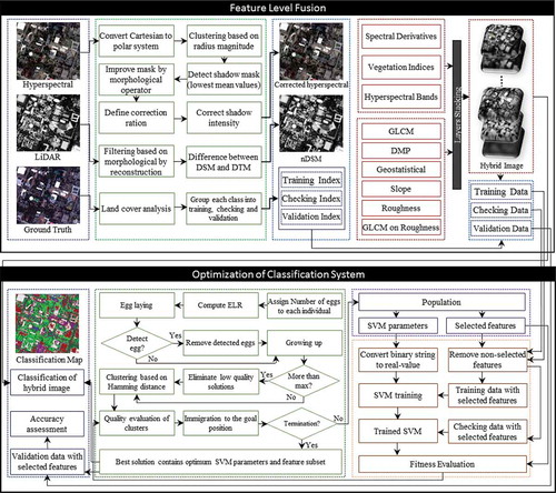
In order to fuse hyperspectral imagery and LiDAR data, a hybrid feature space consisting of structural and spectral features is generated based on LiDAR and hyperspectral data, respectively. According to the stability of SVM in high dimensional space (Melgani & Bruzzone, 2004), SVM is selected as classifier. In order to optimize classification of this hybrid feature space based on SVM, optimized values for its parameters and appropriate feature subsets should be selected. For this purpose, the cuckoo search is applied to determine SVM parameters and selection of features simultaneously.

Preprocessing

In order to prepare data for the classification procedure and improve the classification performance, the preprocessing is required which is performed for both hyperspectral imagery and LiDAR data.

Hyperspectral preprocessing

Since our dataset contains cloud shadow areas, the preprocessing is applied to remove cloud shadow from hyperspectral imagery. Shadows cause changes in the spectral signature shape in addition to decrease in intensity. In order to remove cloud shadow in hyperspectral image (with N bands), the N-dimensional Cartesian coordinate system transforms to polar coordinate system with N − 1 angles and a radius. The radius is equivalent to the spectral illumination value. All pixels are clustered based on their radiuses magnitudes by K-means algorithm. Then, the cluster with the lowest mean value is selected as a shadow class. As detecting cloud shadow is the concern, the morphological operators are applied on shadow mask to remove small pixel and also fill the gaps in the shadow areas. The ratio of the resulting non-shadow-to-shadow mean vectors is used as a correction ratio to the shadow-area intensity (Ashton, Wemett, Leathers, & Downes, 2008).

LiDAR-derived DSM preprocessing

In order to analyze the DSM accurately, nDSM is extracted from DSM by morphological grayscale reconstruction (Arefi & Hahn, 2005). For this purpose, the disk-shaped structuring element (SE) is used and its size is defined based on the object’s size in the dataset.

Hybrid feature space generation

Feature space is a key element in the decision-making system that directly influences the performance (computation complexity, processing time) and the accuracy of results. Therefore, at the first step of the proposed method, an enlarged feature space based on hyperspectral imagery and LiDAR data is generated.

Spectral features

Hyperspectral original bands include rich sources of spectral information but some indicators such as vegetation indices and spectral derivatives may give additional information. Therefore, 30 vegetation indices are computed to discriminate vegetation classes from other classes. Table 1 presents the vegetation indices and their corresponding derivation equations (Hamzeh, Naseri, AlaviPanah, Mojaradi, & Bartholomeus, 2013).

Table 1. Vegetation indices from hyperspectral image. R_x is the reflectance at x nm.

Name	Equation
Normalized difference vegetation index
Simple ratio
Enhanced vegetation index (EVI)
Atmospherically resistant vegetation index (ARVI)
Sum green index (SGI)
Red edge normalized difference vegetation index
Modified red edge simple ratio index
Modified red edge normalized difference vegetation index
Vogelmann red edge index 1
Vogelmann red edge index 2
Red edge position index (REPI)	wavelength of steepest slope within the range 690–740 nm
Photochemical reflectance index (PRI)
Structure insensitive pigment index (SIPI)
Red green ratio index (RGRI)
Plant senescence reflectance index
Carotenoid reflectance index 1
Carotenoid reflectance index 2
Anthocyanin reflectance index 1
Anthocyanin reflectance index 2
Modified simple ratio
Renormalized difference vegetation index
Soil-adjusted vegetation index (SAVI)
Modified SAVI
Modified chlorophyll absorption ration index (MCARI)
MCARI1
MCARI2
Triangular vegetation index (TVI)
Modified TVI (MTVI)
MTVI2
Water band index

Derivatives of spectral reflectance signatures can capture salient features of different land-cover classes. Derivatives are estimated using a finite divided difference approximation algorithm with a finite band separation (Bao, Chi, & Benediktsson, 2013). The first-order spectral derivative can thus be defined by Equation (1).

(1)

where and are the wavelengths corresponding to bands l and k, and and are the spectral reflectance values corresponding to the wavelengths and , respectively. Here, it is assumed and .

Finally, by merging with the original hyperspectral bands, vegetation indices, and spectral derivatives, the spectral feature space is generated.

Structural features

nDSM provides height information; however, more structural features should be generated to improve its ability in discrimination between classes. In order to analyze the nDSM, several spatial and structural types of features are computed.

Gray-level co-occurrence matrices (GLCM) approach is applied to extract 16 second-order statistical textural features including variance, homogeneity, contrast, entropy, dissimilarity, sum average, angular second moment, maximum probability, inverse difference moment, sum entropy, sum variance, difference variance, correlation, difference entropy and two information measures of correlation (Haralick, Shanmugam, & Dinstein, 1973).

Roughness is another structural feature which is extracted from nDSM. The terrain roughness is parameterized by the standard deviation of the detrended z-coordinates of the neighborhood. The plane is fitted to each neighborhood by the least square method and then the standard deviation of detrended height is determined. Texture analysis on the roughness map is also performed to better evaluate the analysis of roughness (Whelley, Glaze, Calder, & Harding, 2014). Moreover, the slope of each neighborhood in the nDSM is computed by applying the normal vector for the obtained plane which leads to a contribution of the slope feature to the structural feature space.

Differential Morphological Profile (DMP) feature extraction method is carried out to define the shape and size of objects based on a morphological operator by reconstruction. Let and be the respective morphological opening and closing operators by reconstruction using . Moreover, Π and Π be the opening and closing profile at the pixel x of nDSM which is defined by Equations (2) and (3), respectively.

(2)

(3)

The DMP is defined as a vector where the measure of the slope of the opening–closing profile is stored for every step of an increasing SE series. The derivative of opening profile and the derivative of closing profile are defined by Equations (4) and (5), respectively.

(4)

(5)

Generally, the derivative of morphological profile or DMP can be written as Equation (6):

(6)

with n equal to the total number of iteration, c = 1, …, 2n, and |n − c| is the size of the morphological transform (Benediktsson, Pesaresi, & Arnason, 2003).

Geostatistical features describe the dependence of spatially correlated point x and x + h, where h is the lag interval within a distribution of regionalized variable Z(x). Three descriptors consisting of Semi-variogram, Madogram, and Rodogram are computed by Equations (7–9), respectively (Chica-Olmo & Abarca-Hernández, 2004).

(7)

(8)

(9)

where N(h) is the number of lag pairs separated by h.

Finally, by merging the nDSM, its textural features, roughness and its textural features, slope, DMP and geostatistical descriptors, the structural feature space is generated.

Classification based on SVM

SVM is a learning technique derived from statistical learning theory. The SVM classification is done by calculating an optimal separating hyperplane that maximizes the margin between two classes. If samples are not separable in the original space, kernel functions are used to map data into a higher dimensional space with a linear decision function (Abe, 2010).

Given a dataset with n samples where is a feature vector with k components and denotes the label of . The SVM looks for a hyperplane in a high dimensional space, able to separate the data from classes ‏1 and −1 with a maximum margin. w is a weight vector, orthogonal to the hyperplane, b is an offset term and is a mapping function which maps data into a high dimensional space to separate data linearity with a low training error. Maximizing the margin is equivalent to minimizing the norm of w. Thus, by solving the following minimization problem, SVM will be trained:

(10)

where C is a regularization parameter that imposes a trade-off between the number of misclassification in the training data and the maximization of the margin and are slack variables. The decision function obtained through the solution of the minimization problem in Equation (10) is given by

(11)

where the constants are called Lagrange multipliers determined in the minimization process. SV corresponds to the set of support vectors, training samples for which the associated Lagrange multipliers are larger than zero. The kernel functions compute dot products between any pair of samples in the feature space. According to capacity of Gaussian Radial Basic Function kernel in high dimensional feature space, it is used in this paper which is defined by Equation (12).

(12)

In the proposed method, classifier plays an important role in evaluation of the fitness function where SVM is trained by training data and trained SVM is evaluated by unseen data.

Simultaneous SVM parameter determination and feature subset selection based on cuckoo search

Cuckoo search is a branch of swarm intelligence algorithms which is inspired by the brood parasitism of cuckoos in the nature. Cuckoos lay their eggs in the nest of host bird. In some case, hosts discover the foreign eggs and throw them away; otherwise, they grow up and become mature. Then, matured cuckoos make some groups with different quality. The position of best group will be the destination for the other cuckoos and they will immigrate there. They live near the best position and start to lay eggs in their neighborhood. These steps are repeated till all cuckoos are gathered near the same place (Yang & Deb, 2009).

For applying cuckoo search in optimization problem, candidate solutions correspond to the position of egg-laying which is called habitat. In our optimization problem, a habitat is a binary string which consists of four parts: spectral features, structural features, regularization parameter and kernel parameter. The lengths of the first and second components are equal to the dimension of spectral feature space (n_Spec) and structural feature space (n_Struc), respectively. Regularization and kernel parameters are real-valued and transform to binary coding for consistency with the binary nature of the feature selection process. The length of regularization (n_c) and kernel parameters (n_k) depends on the range of the parameters and the required precision.

The first and second parts of the binary string of the solution define which feature should be selected by assigning ‘1’ in the ith bit. If the value is ‘0’ in the ith feature in the hybrid feature space, the feature must be discarded. For the determination of the SVM parameters, the binary format of the third and fourth parts of the solution converts to a real-value, expressed by Equation (13).

(13)

where p is the real value of the bit string, min_p and max_p are minimum and maximum values of the parameter p, determined by the user, l is the length of the bit string (for each parameter), and d is a decimal value of the bit string.

Results may have fewer selected features and a higher classification accuracy. The combination of classification accuracy and the number of selected features constitutes the evaluation function. Multiple criteria problems can be solved by creating a single objective fitness function that combines the two goals into one. The objective function is defined by Equation (14).

(14)

where f is the fitness value, is a constant parameter in [0,1], accuracy is obtained by kappa coefficient and N_f is the number of selected features.

According to the optimization part of Figure 1, the candidate solutions are generated which are formed randomly at the first iteration and each habitat is evaluated by Equation (14). Then, the number of eggs are assigned to each habitat and cuckoos lay eggs within a maximum distance from their habitat which is called egg laying radius (ELR) and computed by Equation (15).

(15)

where is constant parameter and is the maximum number of bits that can change. ELR defines the number of bits which should be changed. According to ELR and current candidate solutions, eggs are laid in new positions (by changing bits randomly). Then, some eggs which are detected by host should be removed. For this purpose, p% of eggs with lower quality are defined and eliminated. The remaining habitats are clustered based on K-means algorithm which uses Hamming distance to compute dissimilarity between solutions. Then, their mean fitness function values are calculated and the maximum value of these mean profits defines the goal group and consequently that group’s best solution is the new destination for the immigrant of other solutions. Equation (16) is applied to compute new candidate solutions.

(16)

where is ith candidate solution in tth iteration, is the best habitat in the goal group, is the constant parameter that defines the deviation from straight movement and the next position of cuckoos are determined based on . Since the proposed habitat representation is binary, the new position of habitat should transform to binary string which is done as follows:

(17)

(18)

where is dth variable of ith habitat (), is a vector of random numbers drawn from a uniform distribution between 0 and 1.

Due to the fact that size of cuckoo population does not exceed a confine in nature, a number of N_max is considered which controls and limits the maximum number of solutions. In the cuckoo search algorithm, only N_max number of cuckoos survive that have better fitness values and they form the new population.

These steps are repeated until maximum iteration is satisfied and fitness function (including classification accuracy and dimensionality of feature space) is improved iteratively. After achieving the optimum feature subset and SVM parameters based on cuckoo search, results should be evaluated. The kappa coefficient and the overall accuracy are usually used to determine the classification accuracy. 5-fold cross-validation is also computed to determine the generalization ability of the proposed method. Moreover, the K_hat index is applied to measure the accuracy of each class. These criteria were used to compare classification results and were computed by using the confusion matrix. Furthermore, the statistical significance of differences was computed by using McNemar’s test, which is based upon the standardized normal test statistic (Fauvel, Benediktsson, Chanussot, & Sveinsson, 2008).

(19)

where indicates the number of samples classified correctly by classifier 1 and incorrectly by classifier 2. The difference in accuracy between classifiers 1 and 2 is said to be statistically significant if |Z| > 1.96. The sign of Z indicates whether classifier 1 is more accurate than classifier 2 (Z > 0) or vice versa (Z < 0).

Experimental results

To evaluate the performance of the proposed method, experiments are performed on compact airborne spectrographic imager (CASI) hyperspectral imagery and LiDAR-derived DSM acquired by the NSF-funded Center for Airborne Laser Mapping, both at the same spatial resolution (2.5 m). Datasets are acquired over the University of Houston campus and its neighboring area which cover approximately 870 × 4700 m² (Figure 2).

Figure 2. Datasets (a) hyperspectral imagery (bands 65, 39, 11); (b) DSM derived from LiDAR data.

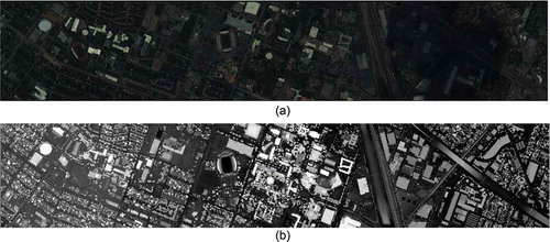
The hyperspectral imagery consists of 144 spectral bands in the spectral range between 380 and 1050 nm and the corresponding co-registered DSM consists of elevation in meters above sea level (Geoid 2012A model). The hyperspectral imagery was acquired on 23 June 2012 between 17:37:10 and 17:39:50 UTC. The average height of the sensor above ground was 5500 ft. The LiDAR data was acquired on June 22 2012, between 14:37:55 and 15:38:10 UTC. The average height of the sensor above ground was 2000 ft (Debes et al., 2014).

The studied area composed of 10 objects: healthy grass, synthetic grass, stressed grass, tree, soil, water, road and highway, parking lot, residential buildings, and commercial buildings. Ground truth samples are randomly divided into training, testing and validation datasets, where Table 2 presents the number of samples in them. Among 10 classes, tree, residential and commercial are placed in the “3D objects” group, where fusion of LiDAR and hyperspectral data may improve classification results. For “2D objects”, hyperspectral data are an efficient tool for discrimination among them. However, 2D objects are commonly grouped as ground level in LiDAR data but the data are also useful in separating 2D and 3D objects.

Table 2. Number of training, testing and validation data for each class.

	3D objects			2D objects
Class	Tree	Residential	Commercial	Healthy grass	Stressed grass	Synthetic grass	Soil	Water	Road and highway	Parking lot
#Training	12	13	12	13	13	12	12	12	35	23
#Test	60	62	61	63	60	61	59	58	180	120
#Validation	116	121	118	122	117	119	115	112	350	233

Preprocessing

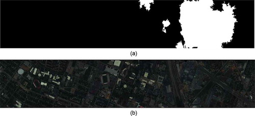
Figure 2(a) shows that there are large areas in the scene with the cloud shadow which degrade the classification performance. In the preprocessing step, the shadow mask is created and its effect is removed from the hyperspectral imagery (Figure 3).

Figure 3. (a) Cloud shadow mask; (b) hyperspectral imagery with removed shadow.

Morphological operators by reconstruction are applied on the DSM (Figure 2(b) to generated nDSM (Figure 4).

Figure 4. nDSM.

Feature space generation

The generation of feature space is performed by processing both hyperspectral imagery and LiDAR data. The hyperspectral image was acquired by the CASI sensor and it has 144 bands which provide a rich source of spectral information. Moreover, 30 vegetation indices are computed (Table 1). Derivatives of spectral reflectance also are computed with step length of five bands which leads to adding 139 features to spectral feature space. Consequently, the spectral feature space is composed of 313 descriptors.

The nDSM derived from DSM data is the source of structural information. Texture analysis of nDSM is performed based on GLCM features; 16 descriptors are extracted, roughness map and its 16 textural descriptors and slope as further descriptor are also computed. Moreover, DMP is generated by applying disk structure element size of SE = 3–15 pixels with step of 2 pixels, which yields to 14 features. Finally, geostatistical descriptors are generated by window size and lag of 15 and [1, 1], respectively. Therefore, the structural feature space is generated by merging all these 52 features.

By merging spectral and structural feature space, a hybrid image is generated that contains rich information content for each pixel and forms our feature space with 365 features for pixel-based classification.

SVM classification results

SVM classifier is applied to classify the hybrid feature space. The SVM classification was done by using the A Library for Support Vector Machine (LIBSVM) through its Matlab interface (Chang & Lin, 2001).

In order to evaluate the potential of hyperspectral images and LiDAR data for the classification of urban areas, standard SVMs are first applied to each dataset separately, then to hyperspectral and LiDAR data, spectral and structural feature space, and finally to the hybrid image. SVM parameters have significant influence on its performance using all features. Therefore, grid search is applied to determine SVM parameters. In grid search, regularization and kernel parameters range within [2¹, …, 2¹⁰] and [2^–5, …, 2⁵], respectively.

The results of SVM classification along with determined parameters for six datasets are presented in Table 3. Obtained results show that LiDAR data are not accurate enough to classify the dataset; on the other side, hyperspectral data show comparable results with respect to the hybrid image. However, the hybrid image still exhibits a superior performance through the fusion of two datasets with different information content.

Table 3. Classification accuracy and SVM parameters for grid search.

Data	C	Gamma	Test data		Validation data		Cross-validation (%)
			Kappa	Overall accuracy (%)	Kappa	Overall accuracy (%)
Hyperspectral	1024	1	0.859	87.63	0.841	86.08	90.4
LiDAR	1024	32	0.236	33.8	0.209	31.39	35.23
Hyperspectral + LiDAR	128	4	0.86	87.76	0.854	87.20	94.84
Spectral features	1024	2	0.876	89.16	0.867	88.31	91.89
Structural features	128	2	0.74	77.17	0.736	76.89	76.89
Hybrid image	128	0.062	0.898	91.1	0.897	91	95.64

The highest classification accuracy for the hybrid image proves the ability of proposed feature-level fusion. However, using LiDAR data in addition to hyperspectral imagery show comparable result to hybrid image. It is due to redundancy in the hybrid feature space that decreases the classification performance. Moreover, the obtained results show spectral and structural features improve classification accuracy in comparison with hyperspectral imagery and LiDAR data, respectively, that confirm efficiency of feature extraction methods.

Figure 5 illustrates the results of McNemar’s test of hybrid image with respect to hyperspectral imagery, LiDAR data, hyperspectral and LiDAR data, spectral and structural features.

Figure 5. McNemar’s test for hybrid image with respect to hyperspectral imagery, LiDAR data, hyperspectral and LiDAR data, spectral and structural features.

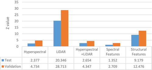
Analyzing Figure 5 reveals also in the statistical analysis the hybrid image improves the result of classification in comparison to raw individual dataset and their feature extracted space. More detailed results for the assessment of the behavior of each class are presented in Figures 6 and 7. The accuracy for each class for hyperspectral, LiDAR, hyperspectral and LiDAR, spectral features, structural features and hybrid image are calculated. The accuracy of 3D classes is shown in Figure 6 which confirms our hypothesis about improving classification performance using a hybrid image.

Figure 6. Classification results for 3D objects based on SVM classifier.

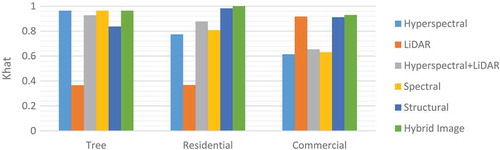
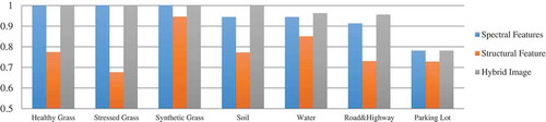
Figure 7. Classification results for 2D objects based on SVM classifier.

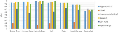
Figure 7 demonstrates the accuracy of hyperspectral, LiDAR, hyperspectral and LiDAR, spectral features, structural features, and hybrid image data for 2D classes in SVM classification.

A closer look at this figure shows that the hybrid image achieves the same/superior accuracy for most classes; however, there are several redundant and inconsistence features which degrade classification performance in stressed grass and parking lot classes.

Simultaneous parameter determination and feature selection based on cuckoo search

Although the hybrid image improves the classification accuracy, there are several correlated and redundant features which degrade classification performance. On the other side, the SVM parameters are important elements in classification. SVM parameters influence the feature subset selection and vice versa; therefore, in this section, simultaneous SVM parameters tuning and feature subset selection based on cuckoo search is performed. Table 4 contains important values for the cuckoo search. The length of the binary string is proportional to the complexity and dimensionality of the search space. Other parameters are tuned by experience.

Table 4. Parameter values of cuckoo search.

Parameters	Value
	385
Number of cuckoo	30
	50
Number of cuckoo’s egg	[1,5]
p	10%
	1
	0.5
Number of cluster	3
	385
Maximum iteration	300

Figure 8 depicts the convergence plots for the cuckoo search procedures in spectral and structural features and hybrid image. The fitness value for the best individual in each generation is shown. The weight parameter in objective function (Equation 14) is set to which considers 80% of fitness to accuracy and 20% to dimensionality of feature space.

Figure 8. Fitness value for global best in each iteration of cuckoo search.

This figure shows that the improvement in fitness value (i.e. classification performance) is superior for the hybrid image with respect to the spectral and structural features. As mentioned, the fitness function consists of two components: kappa coefficient and feature space dimension. In order to evaluate the variety in classification accuracy, Figure 9(a) shows the kappa coefficient for global best depending on iterations.

Figure 9. (a) Kappa coefficient; (b) number of selected features for global best in each iteration of cuckoo search.

For assessment of the variety of feature space dimensionality in the optimization process, Figure 9(b) presents the number of selected features by global best depending on iterations. Moreover, this figure demonstrates that the smaller feature subset size (127 features) is selected for hybrid image with respect to aggregation of selected spectral features (120) and selected structural features (25) separately.

The computation time of the proposed method is influenced by population size, maximum iteration and complexity of cuckoo search. According to low computation complexity (Equations 15–18) and high convergence speed of the cuckoo search (Figure 8), the optimization process has reasonable computation times.

The obtained results yield improvements in classification accuracy and remarkable decrease in the feature space dimension. Table 5 summarizes the selected features for the proposed method for spectral feature space, structural feature space and hybrid image.

Table 5. Selected features in proposed method.

Dataset	# Selected features	Selected spectral feature	Selected structural features
Spectral feature space	134	71 Hyperspectral bands 4 Vegetation indices 59 Spectral derivative	-
Structural feature space	25	-	10 GLCM descriptors 13 DMP components 2 Geostatistical descriptors
Hybrid image	127	52 Hyperspectral bands 7 Vegetation indices 47 Spectral derivative	11 GLCM descriptors 10 DMP components

In order to evaluate the strength of each selected feature category (Table 5), leaving one category out of analysis for hybrid image is carried out. For this purpose, the classification of the proposed method is compared with the classification of data with removed one feature category. Figure 10 shows McNemar’s test for statistical analysis of difference between the proposed method with other scenarios (such as selected features without hyperspectral bands or selected features without DMP).

Figure 10. Z-values for leave one category out analysis.

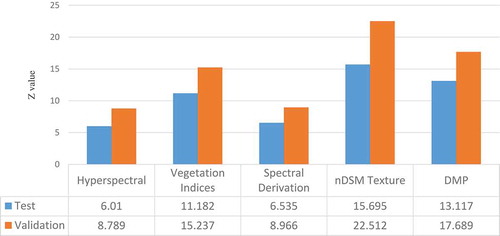
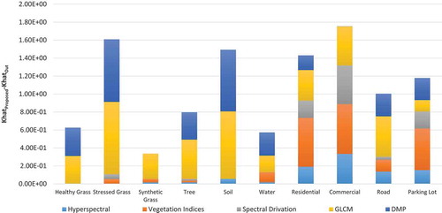
Figure 10shows that removing each type of features statistically decrease the classification performance. Figure 11 illustrates the effect of each feature category on certain classes. It shows decreasing each class accuracy by eliminating feature categories.

Figure 11. Effect of each feature category on all classes accuracies.

Table 6 contains the number of selected features, as well as the values of regularization and kernel parameters and the classification accuracy for the test and validation datasets, determined with the proposed method for spectral and structural and hybrid feature space.

Table 6. Results of simultaneous feature selection and parameter determination based on cuckoo search for spectral and structural feature space and hybrid image.

Data	#Spectral	#Structure	C		Test data		Validation data		Cross-validation (%)
					Kappa	Overall accuracy (%)	Kappa	Overall accuracy (%)
Spectral features	134	–	1021.003	1.906	0.897	90.94	0.872	88.77	91.41
Structural features	–	25	328.68	1.026	0.809	83.16	0.779	80.5	86.65
Hybrid image	106	21	501.511	0.162	0.943	95.03	0.939	94.68	96.88

It reveals that applying the proposed method on the hybrid image yields the best performance in comparison to each dataset separately. Moreover, the total number of selected features in spectral and structural feature space is higher than for the hybrid image (Table 6). For detailed evaluation of results, per class accuracy assessments are presented in Figures 12 and 13 for 3D and 2D classes, respectively.

Figure 12. Classification results for 3D objects based on proposed method.

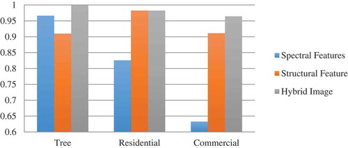
Figure 13. Classification results for 2D objects based on proposed method.

Figure 12 shows that classification of the hybrid image based on the proposed classification system achieves already good results for 3D objects (higher than 96%). Moreover for these classes, height information in hybrid image lead to more accurate results with respect to classification of only spectral features.

As Figure 7 shows, fusion of LiDAR data and hyperspectral image degrades classification performance for some classes in comparison to classification of hyperspectral data. However, by selecting the optimum feature space and tuning SVM parameters simultaneously, this problem is fixed and 2D classes have the same/better accuracy using the optimized hybrid image in comparison to only using the spectral feature space (Figure 13).

Statistical analysis of the result of optimization process is performed by McNemar’s test. Figure 14 presents the Z-value for the result of simultaneous SVM parameter determination and feature selection versus the result of standard SVM.

Figure 14. McNemar’s test for result of optimization based on cuckoo search with respect to standard SVM results.

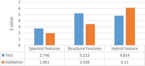
Figure 14 shows that all Z-values for both test and validation data are above 1.96 which prove the statistically significant improvement of the proposed optimization process in comparison with standard SVM.

The generation of a hybrid image followed by an optimization of the classification system improves the classification performance of only hyperspectral imagery by about 6%. The proposed method eliminates 238 redundant features of the hybrid image; therefore, it not only reduces the dimensionality of the feature space (and decreases computation complexity) but also improves the general and classification accuracy which yields a reliable classification system for hybrid image data.

A comparison between the accuracy of each class in standard SVM and the proposed method reveals that for all classes better accuracy or same accuracy is achieved based on the proposed method (considering also the application of a smaller feature subset). Moreover, the improvement in accuracy of two important classes in urban areas, residential and commercial is considerable.

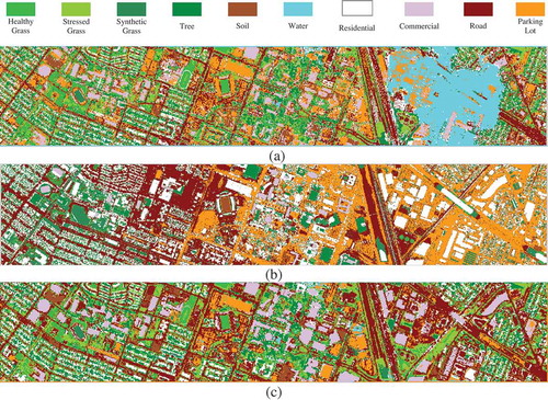
The obtained results prove the ability of the proposed method in fusion of hyperspectral imagery and LiDAR data in classification of urban areas with a large number of classes. Hyperspectral imagery gains acceptable results, although it is not successful in classification of buildings (residential and commercial). Nevertheless, buildings are one of the most important objects in urban areas, so LiDAR data improve significantly the classification accuracy of these classes. The proposed method efficiently fuses these two sources of data to produce accurate classification results. Figure 15 shows the classification map based on hyperspectral imagery, LiDAR data and the proposed method.

Figure 15. Classification maps for (a) hyperspectral; (b) LiDAR and (c) proposed method.

Conclusion

This study investigates the framework for optimization of a hybrid classification system to fuse hyperspectral and LiDAR data based on cuckoo search. Experiments were carried out using CASI hyperspectral image data and a DSM derived from LiDAR data, providing by the IEEE GRSL (Institute of Electrical and Electronics Engineers [IEEE] Geoscience and Remote Sensing Society [GRSS]) Fusion Contest 2013. Several spectral and structural features were extracted from hyperspectral and LiDAR data, respectively. Although SVM is an appropriate classifier for this high dimensional space, its performance is optimized by simultaneous determination of parameters and selection of feature subsets.

The obtained results show that utilizing 3D information from LiDAR data in addition to high spectral information from hyperspectral data improves the classification performance, especially for 3D objects such as trees and buildings (residential and commercial). However, for some classes which exhibit no height difference such as road and grass, there is no meaningful difference between hyperspectral and hybrid feature space.

Optimization of the hybrid classification system based on cuckoo search improves the classification accuracy more than 5% along with the elimination of 235 redundant features. Therefore, the optimum hybrid classification system reaches more accurate results in a less complex space. Per class accuracy is also improved by removing redundant features, and all classes in the hybrid system have better/same accuracy with respect to the results of only hyperspectral/LiDAR data classification.

These are very encouraging results, and we suggest conducting further research, for example, assessment of more textural features from LiDAR data and spectral indices from hyperspectral imagery, using last pulse besides first pulse or full waveform LiDAR data, applying multi-objective optimization method to determine SVM parameters and select the feature subset, automatic determination of cuckoo search parameters (e.g. population size, α and λ) and evaluating the potential of other meta-heuristic algorithms, especially swarm-based optimization algorithms.

Acknowledgments

The authors would like to thank the Hyperspectral Image Analysis group and the NSF-Funded Center for Airborne Laser Mapping (NCALM) at the University of Houston for providing the datasets used in this study and the IEEE GRSS Data Fusion Technical Committee for organizing the 2013 Data Fusion Contest.

Disclosure statement

No potential conflict of interest was reported by the authors.

References

- Abe, S. (2010). Support vector machines for pattern classification (pp. 442 pages). London: Springer-Verlag. doi:10.1007/978-1-84996-098-4
- Arefi, H., & Hahn, M. (2005). A morphological reconstruction algorithm for separating off-terrain points from terrain points in laser scanning data. International Archives of Photogrammetry, Remote Sensing and Spatial Information Sciences, 36(3/W19), 120–236.
- Ashton, E.A., Wemett, B.D., Leathers, R.A., & Downes, T.V. (2008). A novel method for illumination suppression in hyperspectral images. SPIE Defense and Security Symposium: pp. 69660C–69660C. doi: 10.1117/2.1200807.1209.
- Ban, Y., & Jacob, A. (2016). Fusion of multitemporal spaceborne SAR and optical data for urban mapping and urbanization monitoring. Multitemporal Remote Sensing, 20, 107–123. doi:10.1007/978-3-319-47037-5_6
- Bao, J., Chi, M., & Benediktsson, J.A. (2013). Spectral derivative features for classification of hyperspectral remote sensing images: Experimental evaluation. IEEE Journal of Selected Topics in Applied Earth Observation and Remote Sensing, 6(2), 594–601. doi:10.1109/JSTARS.2013.2237758
- Benediktsson, J.A., Pesaresi, M., & Arnason, K. (2003). Classification and feature extraction for remote sensing images from urban areas based on morphological transformations. IEEE Transaction on Geoscience and Remote Sensing, 41(9), 1940–1949. doi:10.1109/TGRS.2003.814625
- Chang, C.C., & Lin, C.J. (2001). LIBSVM: A library for support vector machines. [Online]. Available: http://www.csie.ntu.edu.tw/~cjlin/libsvm.
- Chang, C.I. (2013). Hyperspectral data processing: Algorithm design and analysis (pp. 1135 pages). USA: John Wiley & Sons, Inc. doi:10.1002/9781118269787
- Chica-Olmo, M., & Abarca-Hernández, F. (2004). Variogram derived image texture for classifying remotely sensed images. Remote Sensing and Digital Image Processing, 5, 93–111. doi:10.1007/978-1-4020-2560-0_6
- Dalponte, M., Bruzzone, L., & Gianelle, D. (2008). Fusion of hyperspectral and LIDAR remote sensing data for classification of complex forest area. IEEE Transactions on Geoscience and Remote Sensing, 46(5), 1416–1427. doi:10.1109/TGRS.2008.916480
- Debes, C., Merentitis, A., Heremans, R., Hahn, J., Frangiadakis, N., Van Kasteren, T., Liao, W., Bellens, R., Pizurica, A., Gautama, S., Philips, W., Prasad, S., Qian, D., Pacifici, F. (2014). Hyperspectral and LiDAR data fusion: Outcome of the 2013 GRSS data fusion contest. IEEE Journal of Selected Topics in Applied Earth Observation and Remote Sensing, 7(6), 2405–2418. doi:10.1109/JSTARS.2014.2305441
- Dian, Y., Pang, Y., Dong, Y., & Li, Z. (2016). Urban tree species mapping using airborne LiDAR and hyperspectral data. Journal of the Indian Society of Remote Sensing, 1–9. doi:10.1007/s12524-015-0543-4
- Fauvel, M., Benediktsson, J.A., Chanussot, J., & Sveinsson, J.R. (2008). Spectral and spatial classification of hyperspectral data using SVMs and morphological profiles. IEEE Transactions on Geoscience and Remote Sensing, 46(11), 3804–3814. doi:10.1109/TGRS.2008.922034
- Forzieri, G., Tanteri, L., Moser, G., & Catani, F. (2013). Mapping natural and urban environments using airborne multi-sensor ADS40-MIVIS-LiDAR synergies. International Journal of Applied Earth Observation and Geoinformation, 23, 313–323. doi:10.1016/j.jag.2012.10.004
- Ghamisi, P., Dalla Mura, M., & Benediktsson, J.A. (2015). A survey on spectral–spatial classification techniques based on attribute profiles. IEEE Transactions on Geoscience and Remote Sensing, 53(5), 2335–2353. doi:10.1109/TGRS.2014.2358934
- Hamzeh, S., Naseri, A.A., AlaviPanah, S.K., Mojaradi, B., & Bartholomeus, H.M. (2013). Estimating salinity stress in sugarcane fields with spaceborne hyperspectral vegetation indices. International Journal of Applied Earth Observation and Geoinformation, 21, 282–290. doi:10.1016/j.jag.2012.07.002
- Haralick, R.M., Shanmugam, K., & Dinstein, I. (1973). Textural features for image classification. IEEE Transaction on Systems, Man and Cybernetics, SMC-3(6), 610–621. doi:10.1109/TSMC.1973.4309314
- Hsu, C.W., Chang, C.C., & Lin, C.J. (2003). A practical guide to support vector classification. National Technical Report, Taiwan University.
- Khodadadzadeh, M., Li, J., Prasad, S., & Plaza, A. (2015). Fusion of hyperspectral and LiDAR remote sensing data using multiple feature learning. IEEE Journal of Selected Topics in Applied Earth Observations and Remote Sensing, 8(6), 2971–2983. doi:10.1109/JSTARS.2015.2432037
- Latifi, H., Fassnacht, F., & Koch, B. (2012). Forest structure modeling with combined airborne hyperspectral and LiDAR data. Remote Sensing of Environment, 121, 10–25. doi:10.1016/j.rse.2012.01.015
- Lin, X., & Zhang, J. (2014). Segmentation-based filtering of airborne LiDAR point clouds by progressive densification of terrain segments. Remote Sensing, 6(2), 1294–1326. doi:10.3390/rs6021294
- Liu, L., Pang, Y., Fan, W., Li, Z., & Li, M. (2011). Fusion of airborne hyperspectral and lidar data for tree species classification in the temperate forest of northeast china. 19th International Conference on Geoinformatics, 1-5. doi: 10.1109/GeoInformatics.2011.5981118.
- Liu, Q.J., Jing, L.H., Wang, L.M., & Lin, Q.Z. (2014). A method of particle swarm optimized SVM hype-spectral remote sensing image classification. IOP Conference Series: Earth and Environmental Science, 17(1), p. 012205.
- Liu, X., & Bo, Y. (2015). Object-based crop species classification based on the combination of airborne hyperspectral images and LiDAR data. Remote Sensing, 7, 922–950. doi:10.3390/rs70100922
- Lodha, S.K., Kreps, E.J., Helmbold, D.P., & Fitzpatrick, D. (2013). Aerial LiDAR data classification using Support Vector Machines (SVM). Third symposium on 3D Data Processing, Visualization, and Transmission, 567–574. doi: 10.1109/3DPVT.2006.23.
- Melgani, F., & Bruzzone, L. (2004). Classification of hyperspectral remote sensing images with support vector machines. IEEE Transactions on Geoscience and Remote Sensing, 42(8), 1778–1790. doi:10.1109/TGRS.2004.831865
- Pan, Z., Glennie, C., Fernandez-Diaz, J.C., Shrestha, R., Carter, B., Hauser, D., … Sartori, M. (2016). Fusion of bathymetric LiDAR and hyperspectral imagery for shallow water bathymetry. IEEE International in Geoscience and Remote Sensing Symposium (IGARSS), 3792–3795. doi: 10.1109/IGARSS.2016.7729983.
- Rashedi, E., & Nezamabadi-Pour, H. (2014). Feature subset selection using improved binary gravitational search algorithm. Journal of Intelligent & Fuzzy Systems, 26(13), 1211–1221. doi:10.3233/IFS-130807
- Samadzadegan, F., Hasani, H., & Schenk, T. (2012). Determination of optimum classifier and feature subset in hyperspectral images based on ant colony system. Photogrammetric Engineering and Remote Sensing, 78(12), 1261–1273. doi:10.14358/PERS.78.11.1261
- Shimoni, M., Gustav, T., Christiaan, P., & Jörgen, A. (2011). Detection of vehicle in shadow area using combined hyperspectral and LiDAR data. IEEE International Geoscience and Remote Sensing Symposium, 4427–4430. doi: 10.1109/IGARSS.2011.6050214.
- Sugumaran, R., & Voss, M. (2007). Object-oriented classification of LiDAR-fused hyperspectral imagery for tree species identification in an urban environment. Urban Remote Sensing Joint Event, 1–6. doi:10.1109/URS.2007.371845
- Whelley, P.L., Glaze, L.S., Calder, E.S., & Harding, D.J. (2014). LiDAR-derived surface roughness texture mapping: Application to Mount St. Helens Pumice Plain deposit analysis. IEEE Transactions on Geoscience and Remote Sensing, 52(1), 426–438. doi:10.1109/TGRS.2013.2241443
- Wu, B., & Tang, S. (2015). Review of geometric fusion of remote sensing imagery and laser scanning data. International Journal of Image and Data Fusion, 6(2), 97–114. doi:10.1080/19479832.2015.1024175
- Yang, X.S., & Deb, S. (2009). Cuckoo search via Lévy flights. IEEE World Congress on Nature & Biologically Inspired Computing (Nabic), 210–214. doi:10.1109/NABIC.2009.5393690
- Zhang, C., & Qiu, F. (2012). Mapping individual tree species in an urban forest using airborne LiDAR data and hyperspectral imagery. Photogrammetric Engineering and Remote Sensing, 78(10), 1079–1087. doi:10.14358/PERS.78.10.1079