Mapping land use with using Rotation Forest algorithm from UAV images

ABSTRACT

The aim of this study is to test the performance of the Rotation Forest (RTF) algorithm in areas that have similar characteristics by using Unmanned Aerial Vehicle (UAV) images for the production of most up-to-date and accurate land use maps. The performance of the RTF algorithm was compared to other ensemble methods such as Random Forest (RF) and Gentle AdaBoost (GAB). The accuracy assessments showed that the RTF with 84.90% and 93.33% accuracies provided better performance than RF (7% and 4%) and GAB (15% and 11%) in urban and rural areas, respectively. Subsequently, in order to increase the classification accuracy, a majority filter was applied to post-classification images and the overall classification accuracy of the RFT was increased approximately up to 3%. Also, the results of classification were also analysed using the McNemar test. Consequently, this study shows the success of the RTF algorithm in the classification of UAV images for land use mapping.

KEYWORDS:

• Rotation Forest
• Random Forest
• Unmanned Aerial Vehicle
• classification
• McNemar test

Introduction

Planners, scientists, resource managers and decision makers commonly use updated land use data in problem analysis aimed towards the development of environmental and life conditions (Anderson, Hardy, Roach, & Witmer, 1976; Rozenstein & Karnieli, 2011). When obtaining land use/cover data, which represent the earth surface as a map, remote-sensing technology is considered a very useful tool (Foody, 2002; Rozenstein & Karnieli, 2011; Solaimani, Arekhi, Tamartash, & Miryaghobzadeh, 2010; Sonobe, Tani, Wang, Kobayashi, & Shimamura, 2014; Zhang & Zhu, 2011). However, spatial and spectral resolutions of remote-sensing data, which increased in accordance with advancing technology, led people to prefer to use them in other applications as well, such as urban and environmental applications. In order to accurately process the heterogeneity of the urban land cover, high spatial and spectral resolution images are specially preferred (Qian, Zhou, Yan, Li, & Han, 2015). Laliberte, Herrick, Rango and Winters (2010) indicated that low-cost Unmanned Aerial Vehicle (UAV), which ensures a high-spatial resolution image independent from the pilot, may be an alternative to rapidly generate the land use maps of these areas for its ability to obtain the most up to land use data for the area desired. Image classification is the most commonly used remote-sensing technique which is used to generate land use maps by analysing high-resolution remote-sensing data (Agarwal, Vailshery, Jaganmohan, & Nagendra, 2013; Aguilar, Saldaña, & Aguilar, 2013; Duro, Franklin, & Dubé, 2012; Foody, 2002; Jebur, Mohd Shafri, Pradhan, & Tehrany, 2014; Laliberte, Browning, & Rango, 2012; Liu & Yang, 2015; Schneider, 2012).

Richards and Jia (2006) defined that pixel-based image classification is a labelling process which labels the pixels that belong to a given spectral class by using the existing spectral data. [A “salt and pepper” effect is generally observed in the maps generated using this approach (Sun, Heidt, Gong, & Xu, 2003).] This reduces the accuracy of the thematic map. Therefore, this effect may be minimized by applying different filters (spatial, temporal, logistic etc.) to the thematic images obtained from the classification process in order to improve the accuracy of the thematic maps (Khatami, Mountrakis, & Stehman, 2016; Lu, Huang, Liu, & Zhang, 2016; Nex et al., 2015; Stow, Shih, & Culter, 2015; Wang et al., 2015; Zhang, Li, & Zhang, 2016). In recent years, in order to improve overall classification accuracy of individual classifiers (Breiman, 2001; Colkesen & Kavzoglu, 2016; Gislason, Benediktsson, & Sveinsson, 2006; Halmy & Gessler, 2015; Miao, Heaton, Zheng, Charlet, & Liu, 2012; Opitz & Maclin, 1999; Wang, 2006), ensemble approaches such as Random Forest (RF), Rotation Forest (RTF), Boosting and Bagging are commonly used. The ensemble approach is a tree-based learning approach, which utilizes multiple classifiers rather than one single classifier and yields more than one classification result. Among these results, a pixel is labelled according to the class it was most often assigned.

The RTF algorithm is the most recently developed ensemble method. Rodriguez, Kuncheva and Alonso (2006) described RTF as an algorithm which generates classifiers that yield more accurate results when compared to other learning methods such as RF, AdaBoost and Bagging. The RTF approach bases on encourage diversity by using a transformation method to do feature extraction for each classifier (Kotsiantis, 2011). This algorithm generates the data set in a different feature space (principal component analysis [PCA], independent component analysis etc.) and produces multiple classification trees by using the data set transformed to this feature space (Liu & Huang, 2008). Each tree is trained on the data sets present in the transformed feature space (Xia, Du, He, & Chanussot, 2014). Other studies related to image classification support the claim that the classification logic and application of the RTF approach provides more accurate results when compared to other ensemble methods (Du, Samat, Waske, Liu, & Li, 2015; Gaikwad & Pise, 2014; Kuncheva & Rodriguez, 2007; Lasota, Łuczak, & Trawiński, 2012; Liu & Huang, 2008; Xia, 2016; Xia et al., 2014).

In this study, the orthophoto images obtained from high spatial resolution UAV-imaging techniques were used to the most up-to-date and accurate land use maps. The success of RTF was tested and its performance in the pixel-based classification process was compared with other commonly used ensemble methods, such as RF and Gentle AdaBoost (GAB). Lastly, the statistical significance of the results was examined using the McNemar test.

Study area and data set

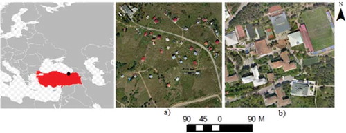
In this study, urban and rural areas that contain spectrally mixed land use classes were selected as study areas. To represent urban area, an area of Trabzon Karadeniz Technical University’s campus was chosen (40°59′54″–40°59′44″N and 39°46′7″–39°46′18″E); to represent rural area, the Hıdırnebi Plateau of Trabzon-Akçaabat district in Turkey (40°58′11″–40°57′56″N and 39°25′51″–39°26′11″E) were selected as pilot study areas (Figure 1).

Figure 1. Study areas: (a) rural and (b) urban.

The collection of high-resolution images were collected using the Gatewing X-100 UAV. In the 150-ha-wide area on the Karadeniz Technical University Campus, 168 images were taken and these images were processed for geo-referencing in Agisoft Photoscan software for urban areas. The Ground Control Points (GCPs) used in processing were coordinated through RTK GPS. In urban area, UAV images were processed in direction with 0.03 m and in direction with 0.05 m error. The image used in urban areas was three banded (red, green, blue) and has 0.05 m spatial resolution. For the rural area of the Hıdırnebi Plateau of Trabzon-Akçaabat district, which was about 661 ha, 741 photos were processed with error rates in x direction with 0.03 m and direction 0.03 m. GCPs which were coordinated through the RTK GPS technique were utilized in the geo-referencing process. This image used in rural areas has three bands and 0.16 m spatial resolution. Orthophoto images were obtained at the end of this processing.

Methodology

Random forest (RF)

RF is a classifier that allows the classification of multiple variables and classes without needing sophisticated models or parameters (Breiman, 2001). Furthermore, RF is superior to many tree-based algorithms (Gislason, Benediktsson, & Sveinsson, 2004; Pal, 2003; Waske, Heinzel, Braun, & Menz, 2007; Watts & Lawrence, 2008).

The principle of RF is splitting each node by using the GINI index to find the best split among randomly selected variables in each node rather than among all the variables and use it for growing the tree (Akar & Güngör, 2015). In RF, Decision Trees (DTs) are trained on the bootstrap samples (random, with replacement) from original training data (Breiman, 2001). Two user-defined parameters are used at this stage. These parameters include the number of variables used in each node to determine the best division () and the number of DTs to be generated (). First, bootstrap samples are formed by randomly selecting 2/3 of the training data set. The remaining 1/3 of the training data set, which is also called out-of-bag data, is used to test the errors. Thereafter, the trees are grown from these randomly selected bootstrap samples without punning. For growing the tree, the best split is determined by the GINI index measurements from a randomly selected number of variables in each node, and then the node is split accordingly (Kim, Im, Ha, Choi, & Ha, 2014). GINI index measures the class homogeneity and can be expressed with the following formula:

(1)

In a given T training data set, the class belonging to a randomly selected pixel is and is the probability that a selected sample belongs to the class of the sample (Pal, 2005). When the GINI index reaches zero, or in other words when a single class remains in each leaf node, the splitting process ends (Watts, Powell, Lawrence, & Hilker, 2011). Depending on the number of trees to be grown, that number is determined by the best split for each node (Liaw & Wiener, 2002).

Gentle AdaBoost

AdaBoost algorithm is an ensemble method that performs the classification process with the weights assigned to difficult-to-classify samples using iterative procedures (Freund & Schapire, 1996). The AdaBoost method grows many classifiers, similarly to RF, and votes them. These two methods differ in the fact that AdaBoost grows the classifiers in an interdependent and consecutive manner whereas RF simultaneously grows many independent classifiers. Weighed data sets at a number equal to T trial are generated as series and classifiers are grown. Final classifiers are determined using C* weighed votes (Bauer & Kohavi, 1999). An equal weight is given for all samples. In each iteration, while the weights of all unclassified samples are increased, the weights of accurately classified samples are decreased. For each individual classifier, one weight is assigned. This weight measures the overall accuracy of the classifier and it is a function of the total weights of the accurately classified samples. Therefore, higher weights are assigned to more accurate classifiers. These weights are used for the classification of the new samples. The AdaBoost algorithm is sensitive to noise in the training data, so Freidman, Hastie and Tibshirani (2000) proposed some new boosting algorithms including GAB, which has proved to solve this problem (Hamdi, Auhmani, Hassani, & Elkharki, 2015). This method is based on the use of the least squares regression method to determine the weight of the AdaBoost algorithm. It aims to minimize the exponential loss function of AdaBoost rather than adapting the data to an estimate of a class probability by using least squares regression (Ho, Lim, Tay, & Binh, 2009).

Rotation forest (RTF)

The RTF algorithm is an ensemble method, which has been proposed by Rodriguez et al. (2006), to encourage both individual accuracy and member diversity within a classifier ensemble (Xia et al., 2014). The RTF algorithm used for classification is a linear transformation method and provides a new performing space within another space (Liu & Huang, 2008). The RTF algorithm is similar to the principle of the RF algorithm in terms of growing multiple trees in classification. However, it differs from RF by using a different feature space such as PCA, to generate the data set. It generates many DTs using the training data sets determined with this feature space. During the training of the DTs using RTF, the training data set is divided into subsets and feature extraction is done by using the feature space selected from each subset. Rodriguez et al. (2006) stated that because of this feature, RTF yields a better classification accuracy compared to RF.

When stands represents for the training data set; represents the classes corresponding to this data set and represents the number of samples, is accepted as the number of samples in training data set and is considered as the number of classes. contains the class values in the range of . Accordingly, the data set is randomly divided into subdivisions that are approximately the same size. The number of DTs present in the RTF is and expressed as L. In the RTF algorithm, and are two user-defined parameters. By using these parameters, the data set used for growing each DT with the RTF method is determined as follows. First, , it is randomly divided into subdivisions. In each subdivision, there are features. Assuming that is the subset that includes features used in the training of the classifier and that is the data set that includes the features present in the in the X data set, new data set is generated using the bootstrap method. Two-third of this data set is used as training data and 1/3 as testing data. PCA transformation is applied to this data set and the covariance matrix is generated. transformation matrix is obtained using the values found in the covariance matrix (Formula 2) (Rodriguez et al., 2006).

(2)

The columns of this matrix are rearranged according to the original features sequence. The new transformation matrix is indicated by . The transformation matrix is used to train classifier. The data set transformed for the classifier is expressed as . According to this approach, all classifiers are provided training in a parallel manner (Liu & Huang, 2008), and the classification is realized. In this step, a trained tree is obtained for each transformed data set and each tree yields a classification result. Among these results, a pixel is labelled by the class to which it was most often assigned. In other words, testing sample belongs to class and the probabilities generated using classifier are . The confidence is calculated for each class using the average combination method (Formula 3).

(3)

, the class with the largest confidence interval, is assigned accordingly (Rodriguez et al., 2006).

Classification process

In the study, for the classification process, a total of seven classes were identified: forest, grass, road, soil, shadow, building1 and building2. The white buildings with roof structures such as steel and concrete were chosen as building1, the red buildings with roof structures such as tiles were chosen as building2. According to these classes, the sample areas were collected for each class from the orthophoto images of the study areas by using Environment for Visualizing Images (ENVI) software. Care was taken to select approximately equal numbers of pixels for each class. In order to generate training samples, Mather (2004) defined the minimum number of pixels required to be collected for each class using ((number of bands) × (number of samples) × (number of classes) formula. Accordingly, the minimum number of samples was determined for these study areas as . Given the number of samples in the ENVI program, training pixels were selected by the image for each class and from each class. Approximately 2700 pixels for urban area and 2500 pixels for rural area were collected, respectively.

Additionally, in order to determine the Separability Index (SI) of the region of interests (ROIs) of the land classes such as forest, grass, road, soil, building1 and building2, Jeffries-Matusita and Transformed divergence measurements in the ENVI 4.7 (ENVI 2009) software. For all classes, SI was calculated and ROIs with a high SI were used in the classification. When values were greater than 1.9, these classes were considered to have good separability (Elsharkawy, Elhabiby, & El-Sheimy, 2012). Two classes were considered to be very poorly separated when ROI pairs were lower than 1.0 (Mei, Manzo, Bassani, Salvatori, & Allegrini, 2014). The formulas (4 and 5) for computing the Jeffries–Matusita distance () are as below:

(4)

(5)

where and are the mean values for the classes and , and are the covariance matrices for classes and , and represents the transpose of a vector (Kumar et al., 2016).

Afterwards, training and test data were created according to the sample grounds chosen on each of the images in the MATLAB software by applying the Random Feature Selection Method. Two-third of training samples were used for training while one-third of them were utilized as testing data. As a result, 12.980 pixels were selected as training data and 6.490 pixels were selected as testing data for rural areas. About 10.199 pixels were selected as training data and 5.099 pixels were selected as testing data for urban area. The user-defined parameters (e.g. and parameters for RF and, and parameters for RTF) were determined by the trial of the user. These optimal turning parameters were used to determine best-performing classification model, and images were classified with the RTF, RF and GAB methods (Figures 2 and 3). In the classification process, MATLAB codes were used. For the RTF, RF and GAB classification approaches, the same training data were utilized.

Figure 2. Classified image for rural area without filter: (a) RTF, (b) RF, (c) GAB, classified image for rural area with majority filter, (d) RTF, (e) RF and (f) GAB.

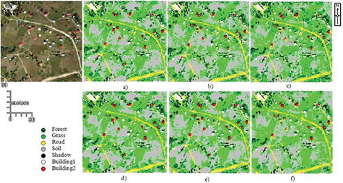
Figure 3. Classified image for urban area without filter: (a) RTF, (b) RF, (c) GAB, classified image for urban area with majority filter, (d) RTF, (e) RF and (f) GAB.

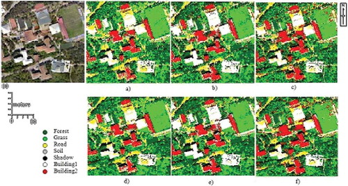
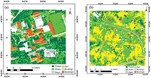
After the post-classification process, misclassified pixels appeared to be the effect of noise in the thematic images. This reduced the quality and the accuracy of the land use map to be generated. Therefore, in order to minimize these effects and increase the accuracy, filtering methods may be used. For this study, a majority filter, which is a spatial filtering, was applied to minimize noise effects. A majority filter is based on the majority rule and applied inside a moving window of size defined by the user (Nex et al., 2015). The noise effect on the images obtained with the classification was likely somewhat eliminated by using the (3 × 3) majority filter (Figures 2 and 3). Lastly, land use maps were generated using the thematic images with the highest classification accuracy for the study areas (Figure 4).

Figure 4. Land use maps: (a) urban and (b) rural.

Accuracy assessment

In literature, there are many studies that examine the number of reference pixels required for the accuracy of analysis. A majority of the investigators used approaches based on binomial distribution for the calculation of the number of required reference pixels. The equations applied to this distribution used the rate of correctly classified samples. However, this technique is not sufficient to determine the number of reference pixels required for the error matrices. This is explained by the fact that the error matrices contained both correctly classified and misclassified samples (Congalton & Green, 1999). So, Congalton and Green (1999) proposed an approach based on multinomial distribution for the calculation of the number of reference pixels that would be enough to generate an error matrix for the accuracy of analysis. They offered the following multinomial distribution equation to calculate the number of required reference pixels for the accuracy of the classification (Equations (6) and (7)):

(6)

(7)

In Equations (6) and (7), represents the number of reference pixels, is the distribution rate of single degree of freedom, is the number of classes, shows the area covered by class which is the ratio of the area covered by the class on the map, is the confidence interval and is the required accuracy. If we wish to precisely determine the number of reference pixels, and information in hand details are present, Equation (6) would be used. In the study, a total of 735 points were produced on an image for 7 classes, using a stratified random method based on the areas covered by the classes. These points were used to analyse the accuracy of the classified thematic images. The accuracy of each classification result was assessed using an error matrix and statistics of the percentages of accuracy were calculated based upon the error matrix. According to Pontius and Millones (2011), Kappa attempts to compare accuracy to a baseline of randomness. However, randomness is not a reasonable alternative for map construction. So, they recommend the use of two other parameters, which are quantity and allocation disagreements. Given this judgement, the κ_quantity and κ_allocation were also calculated for each classified image for post-classification accuracy assessment.

For the statistical significance of the correlation across the classification accuracies, McNemar statistical test based on the table was used. In this test, the following equation is used (Foody, 2004):

(8)

where is the number of correctly classified pixels with a first classifier but misclassified pixels with a second classifier and is the number of misclassified pixels with second classifier but correctly classified pixel.

Result and discussion

In order to evaluate the performance of the RTF classifier compared to the RF and GAB ensemble methods, the error matrices obtained from the accuracy analysis were examined. First, when the error matrices calculated for the urban and rural areas in the RTF were examined, RTF showed a better performance compared to other ensemble methods with overall classification accuracies and kappa values [κ_quantity (0.97), κ_allocation (0.94)] of 93.33%, and kappa values [κ_quantity (0.89), κ_allocation (0.88)] of 84.90%. In urban areas, the higher number of the pixels with similar spectral properties compared to rural areas negatively affected the classification accuracy.

When the error matrices for rural area were examined, misclassified pixels were observed in the classes with similar spectral reflectance values. For example, the road class has similar spectral specifications with building1 and the soil classes. Concrete roads are confused with concrete buildings and soil roads with soil class. The same was observed in the forest and grass classes as well. In the grass and soil classes, in areas with sparse grass, grass pixels were confused with the soil class. When the accuracy of each class was examined, RTF that had a producers’ accuracy close to that of RF represented the forest class, grass class and building1 class better by 4%, 8% and 11% when compared to RF. RF provided a better classification accuracy by 3% and 1% in road and soil classes, respectively. For the users’ accuracy, RTF was more successful in the forest, grass, road and soil classes by 6%, 3%, 8% and 13%, respectively. In building1 class, RF showed higher classification accuracy by 6% compared to RTF (Table 1).

For the urban area, when the error matrices present in Table 2 were examined, it was found that most commonly confused classes were forest and grass, road and building1, and soil and building2. Similarly to rural area, white buildings with concrete and tin roofs were confused with concrete roads and the buildings with brick roof present in the building2 class were confused with the soil class. In terms of producers’ accuracy, RTF was 7%, 13%, 30% and 30% in the forest, grass, road and soil classes compared to RF, respectively, whereas RF classified building1 class and building2 class 14% and 4% better, respectively. For the users’ accuracy, RTF generally yielded more successful results. As also seen in terms of the comparison of classification performances, RTF yielded a higher accuracy compared to other methods in both study areas (Table 3). In addition, the majority filter was also applied to post-classification images in order to decrease the effect of noise in the classified images and to increase the classification accuracy. It was found that using filters resulted in improvements in the classification accuracy from 84.90% to 87.21% for RTF, from 77.69% to 78.50% for RF and from 69.52% to 72.52% for GAB in the urban area and from 93.33% to 94.15% for RTF, from 88.98% to 90.07% for RF and from 82.59% to 83.81% for GAB in the rural area (Table 3). Thereby, the effect of noise on the images was reduced and the quality of the land use maps generated improved.

Table 1. Error matrix of classification for rural area: (a) RTF, (b) RF and (c) GAB.

(a)
			Reference
		Forest	Grass	Road	Soil	Shadow	Building1	Building2	∑Row	P.A. (%)	U.A. (%)
Class	Forest	97	4	0	0	1	3	0	105	91.51	92.38
	Grass	7	94	0	4	0	0	0	105	90.38	89.52
	Road	0	0	98	3	0	1	3	105	86.73	93.33
	Soil	1	6	1	97	0	0	0	105	93.27	92.38
	Shadow	1	0	0	0	104	0	0	105	99.05	99.05
	Building1	0	0	14	0	0	91	0	105	95.79	86.67
	Building2	0	0	0	0	0	0	105	105	97.22	100.00
	∑Column	106	104	113	104	105	95	108	735
Overall accuracy = 93.33%, κquantity = 0.97, κallocation = 0.94.
(b)
			Reference
		Forest	Grass	Road	Soil	Shadow	Building1	Building2	∑Row	P.A. (%)	U.A. (%)
Class	Forest	93	4	0	0	7	3	1	108	87.74	86.11
	Grass	9	86	0	3	0	1	0	99	82.69	86.87
	Road	0	0	102	3	1	7	7	120	90.27	85.00
	Soil	4	14	5	98	0	3	0	124	94.23	79.03
	Shadow	0	0	0	0	97	0	3	100	92.38	97.00
	Building1	0	0	6	0	0	81	0	87	85.26	93.10
	Building2	0	0	0	0	0	0	97	97	89.81	100.00
	∑Column	106	104	113	104	105	95	108	735
Overall accuracy = 88.98%, κquantity = 0.92, κallocation = 0.91.
(c)
			Reference
		Forest	Grass	Road	Soil	Shadow	Building1	Building2	∑Row	P.A. (%)	U.A. (%)
Class	Forest	99	4	0	3	10	5	1	122	93.40	81.15
	Grass	4	84	0	18	0	1	0	107	80.77	78.50
	Road	0	0	102	3	1	11	21	138	90.27	73.91
	Soil	2	16	6	80	0	8	5	117	76.92	68.38
	Shadow	1	0	0	0	94	1	2	98	89.52	95.92
	Building1	0	0	5	0	0	69	0	74	72.63	93.24
	Building2	0	0	0	0	0	0	79	79	73.15	100.00
	∑Column	106	104	113	104	105	95	108	735
Overall accuracy = 82.59%, κquantity = 0.85, κallocation = 0.88.

Table 2. Error matrix of classification for urban area: (a) RTF, (b) RF, (c) GAB.

(a)
			Reference
		Forest	Grass	Road	Soil	Shadow	Building1	Building2	∑Row	P.A. (%)	U.A. (%)
Class	Forest	89	13	3	0	8	0	2	115	83.18	77.39
	Grass	16	85	0	0	0	0	0	101	81.73	84.16
	Road	0	5	79	1	1	16	3	105	90.80	75.24
	Soil	1	0	0	72	0	0	23	96	88.89	75.00
	Shadow	1	0	0	0	99	1	0	101	90.83	98.02
	Building1	0	0	5	2	0	98	2	107	85.22	91.59
	Building2	0	1	0	6	1	0	102	110	77.27	92.73
	∑Column	107	104	87	81	109	115	132	735
Overall accuracy = 84.90%, κquantity = 0.89, κallocation = 0.88.
(b)
			Reference
		Forest	Grass	Road	Soil	Shadow	Building1	Building2	∑Row	P.A. (%)	U.A. (%)
Class	Forest	81	23	2	2	8	0	4	120	75.70	67.50
	Grass	21	72	0	0	0	0	0	93	69.23	77.42
	Road	0	0	53	3	0	1	2	59	60.92	89.83
	Soil	1	2	4	48	0	0	16	71	59.26	67.61
	Shadow	3	0	0	0	96	0	0	99	88.07	96.97
	Building1	1	4	17	7	4	114	3	150	99.13	76.00
	Building2	0	3	11	21	1	0	107	143	81.06	74.83
	∑Column	107	104	87	81	109	115	132	735
Overall accuracy = 77.69%, κquantity = 0.85, κallocation = 0.81.
(c)
			Reference
		Forest	Grass	Road	Soil	Shadow	Building1	Building2	∑Row	P.A. (%)	U.A. (%)
Class	Forest	73	28	2	3	16	8	5	135	68.22	54.07
	Grass	25	61	0	1	0	0	4	91	58.65	67.03
	Road	0	0	43	11	0	13	2	69	49.43	62.32
	Soil	0	0	4	38	0	0	4	46	46.91	82.61
	Shadow	7	0	0	0	91	0	0	98	83.49	92.86
	Building1	1	6	9	10	0	91	3	120	79.13	75.83
	Building2	1	9	29	18	2	3	114	176	86.36	64.77
	∑Column	107	104	87	81	109	115	132	735
Overall accuracy = 69.52%, κquantity = 0.80, κallocation = 0.73.

Table 3. Overall classification accuracies and kappa values for study areas.

(a) For no filtered images
Rural area				Urban area
	Overall acc. (%)	κquantity	κallocation	Overall acc. (%)	κquantity	κallocation
RTF	93.33	0.97	0.94	84.90	0.89	0.88
RF	88.98	0.92	0.91	77.69	0.85	0.81
GAB	82.59	0.85	0.88	69.52	0.80	0.73
(b) For filtered images
Rural area				Urban area
	Overall acc. (%)	κquantity	κallocation	Overall acc. (%)	κquantity	κallocation
RTF	94.15	0.95	0.96	87.21	0.88	0.91
RF	90.07	0.94	0.92	78.50	0.81	0.86
GAB	83.81	0.90	0.86	72.52	0.79	0.78

Finally, the significance of the differences between the accuracies of the classification methods was studied using the McNemar test. As seen in Table 4, according to the result of the McNemar test, , the values for RTF–RF and RTF–GAB were 12.6447 and 53.8407 in the rural area, and 18.6483 and 486,706 in the urban area, respectively. According to Table 4, in the images obtained after the application of the filter, , the values for RTF–RF and RTF–GAB were 9.3444 and 47.6695 in the rural area and 26.1118 and 68.1488 in the urban area, respectively. In the 95% confidence interval of the calculated values, shows that the differences are significant.

Table 4. Assessment of the significance of the difference between ensemble classification results with McNemar test.

(a) The definition of matrix elements used in Equation (8)
		Method2
Allocation		Correct		Incorrect			∑
Method1
Correct
Incorrect
∑
(b) The comparison of RTF–RF and RTF–GAB for study areas
						Total
Rural area	RTF–RF	632	54	22	27	735	12.6447
	RTF–GAB	590	17	96	32	735	53.8407
Urban area	RTF–RF	525	99	46	65	735	18.6483
	RTF–GAB	80	19	543	93	735	486.706
(c) The comparison of filtered RTF–RF and filtered RTF–GAB for study areas
						Total
Rural Area	RTF–RF	632	60	30	13	735	9.3444
	RTF–GAB	595	21	97	22	735	47.6695
Urban Area	RTF–RF	533	108	44	50	735	26.1118
	RTF–GAB	503	30	138	64	735	68.1488

: The number of correctly classified pixels in both cases;  the number of misclassified pixels in both cases; : the number of correctly classified pixels with first classifier but misclassified pixels with second classifier; : the number of misclassified pixels with second classifier but correctly classified pixels with first classifier.

Conclusion

In this study, RTF showed an overall classification accuracy of 84.90% in the urban area and 93.33% in the rural area for the orthophoto images obtained from UAV images. When the overall accuracy of the RTF algorithm was compared with common ensemble methods such as RF and GAB, it was observed that RTF provided better performance than RF and GAB. In urban area, it was found that RTF showed a better performance by approximately 7% and 15% when compared to RF and GAB, respectively. In rural area, RTF was found to be more accurate by 4% and 11% when compared to RF and GAB, respectively. These results showed that the RTF classifier yielded a higher accuracy compared to RF and GAB classifiers. A majority filter used to reduce the effect of the noise in the thematic images obtained after the classification was efficient in increasing the quality and accuracy of the land use maps produced. In addition, the significance of the differences of classification accuracy between RTF and other methods was tested using the McNemar test. These differences were found to be statistically significant. Consequently, the results obtained in this study that investigated the use of the RTF algorithm in the classification of UAV images support the usability of the RTF method in analysing the land use maps to be generated for rural and urban areas.

Acknowledgements

UAV images in this study have been provided by the Department of Geomatics Engineering, Karadeniz Technical University.

Disclosure statement

No potential conflict of interest was reported by the author.

References

- Agarwal, S., Vailshery, L.S., Jaganmohan, M., & Nagendra, H. (2013). Mapping urban tree species using very high resolution satellite imagery: Comparing pixel-based and object-based approaches. ISPRS International Journal of Geo-Information, 2(2013), 220–236. doi:10.3390/ijgi2010220
- Aguilar, M.A., Saldaña, M.M., & Aguilar, F.J. (2013). GeoEYE-1 and WorldView-2 pan-sharpened imagery for object-based classification in urban environment. International Journal of Remote Sensing, 34(7), 2583–2606. doi:10.1080/01431161.2012.747018
- Akar, Ö., & Güngör, O. (2015). Integrating multiple texture methods and NDVI to the random forest classification algorithm to detect tea and hazelnut plantation areas in northeast Turkey. international Journal of Remote Sensing, 36, 442–464. doi:10.1080/01431161.2014.995276
- Anderson, J.R., Hardy, E.E., Roach, J.T., & Witmer, R.E. (1976). A land use and land cover classification system for use with remote sensor data (US Geological Survey, Professional Paper 964). Washington, DC: Government Printing Office.
- Bauer, E., & Kohavi, R. (1999). An empirical comparison of voting classification algorithms: Bagging, boosting, and variants. Machine Learning, 36(1–2), 105–139. doi:10.1023/A:1007515423169
- Breiman, L. (2001). Random Forests. Machine Learning, 45, 5–32. doi:10.1023/A:1010933404324
- Colkesen, I., & Kavzoglu, T. (2016). The use of logistic model tree (LMT) for pixel- and object-based classifications using high-resolution WorldView-2 imagery. Geocarto International, 32(1), 71–86. doi:10.1080/10106049.2015.1128486
- Congalton, R.G., & Green, K. (1999). Assessing the accuracy of remotely sensed data: Principles and practices. Boca Raton: Lewis.
- Du, P., Samat, A., Waske, B., Liu, S., & Li, Z. (2015). Random forest and rotation forest for fully polarized SAR image classification using polarimetric and spatial features. ISPRS Journal of Photogrammetry and Remote Sensing, 105, 38–53. doi:10.1016/j.isprsjprs.2015.03.002
- Duro, D.C., Franklin, S.E., & Dubé, M.G. (2012). A comparison of pixel-based and object-based image analysis with selected machine learning algorithms for the classification of agricultural landscapes using SPOT-5 HRG imagery. Remote Sensing of Environment, 118, 259–272. doi:10.1016/j.rse.2011.11.020
- Elsharkawy, A., Elhabiby, M., & El-Sheimy, N. (2012, March). Improvement in the detection of land cover classes using the Worldview-2 imagery. Paper presented at the ASPRS 2012 Annual Conference, Sacramento, CA.
- ENVI. 2009. ENVI 4.7 User Guide. Research Systems.
- Foody, G.M. (2002). Status of land cover classification accuracy assessment. Remote Sensing of Environment, 80, 185–201. doi:10.1016/S0034-4257(01)00295-4
- Foody, G.M. (2004). Thematic map comparison: Evaluating the statistical significance of differences in classification accuracy. Photogrammetric Engineering and Remote Sensing, 70(5), 627–633. doi:10.14358/PERS.70.5.627
- Freidman, J., Hastie, T., & Tibshirani, R. (2000). Additive logistic regression: A statistical view of boosting. Annals of Statistics, 28, 307–337.
- Freund, Y., & Schapire, R. (1996). Experiments with a new boosting algorithm. In L. Saitta (Ed.). Machine learning: Proceedings of the Thirteenth International Conference (pp. 148–156). San Mateo: Morgan Kaufmann.
- Gaikwad, S., & Pise, N. (2014). An experımental study on hypothyroıd usıng rotatıon forest. International Journal of Data Mining & Knowledge Management Process (IJDKP), 4(6), 31–37. doi:10.5121/ijdkp.2014.4603
- Gislason, P.O., Benediktsson, J.A., & Sveinsson, J.R. (2004, September 20–24). Random forest classification of multisource remote sensing and geographic data. In IEEE International Geoscience and Remote Sensing Symposium Proceedings (IGARSS 2004) (Vol. II), Anchorage, AK. Hoboken, NJ: IEEE International.
- Gislason, P.O., Benediktsson, J.A., & Sveinsson, J.R. (2006). Random forests for land cover classification. Pattern Recognition Letters, 27, 294–300. doi:10.1016/j.patrec.2005.08.011
- Halmy, M.W.A., & Gessler, P.E. (2015). The application of ensemble techniques for land-cover classification in arid lands. International Journal of Remote Sensing, 36(22), 5613–5636. doi:10.1080/01431161.2015.1103915
- Hamdi, N., Auhmani, K., Hassani, M.M., & Elkharki, O. (2015). An efficient Gentle AdaBoost-based approach for mammograms classification. Journal of Theoretical and Applied Information Technology, 81(1), 138–143.
- Ho, W.T., Lim, H.W., Tay, Y.H., & Binh, Q. (2009). Two-stage license plate detection using Gentle Adaboost and SIFT-SVM. In H. Dong & Q. Binh (Eds.), Proceedings of 1st Asian Conference on Intelligent Information and Database Systems (pp. 109–114). doi:10.1109/ACIIDS.2009.25.
- Jebur, M.N., Mohd Shafri, H.Z., Pradhan, B., & Tehrany, M.S. (2014). Per-pixel and object-oriented classification methods for mapping urban land cover extraction using SPOT 5 imagery. Geocarto International, 29(7), 792–806. doi:10.1080/10106049.2013.848944
- Khatami, R., Mountrakis, G., & Stehman, S.V. (2016). A meta-analysis of remote sensing research on supervised pixel-based land cover image classification processes: General guidelines for practitioners and future research. Remote Sensing of Environment, 177, 89–100. doi:10.1016/j.rse.2016.02.028
- Kim, Y.H., Im, J., Ha, H.K., Choi, J.K., & Ha, S. (2014). Machine learning approaches to coastal water quality monitoring using GOCI satellite data. GIScience and Remote Sensing, 51, 158–174. doi:10.1080/15481603.2014.900983
- Kotsiantis, S. (2011). Combining bagging, boosting, rotation forest and random subspace methods. Artificial Intelligence Review, 35, 223–240. doi:10.1007/s10462-010-9192-8
- Kumar, P., Prasad, R., Choudhary, A., Mishra, V.N., Gupta, D.K., & Srivastava, P.K. (2016). A statistical significance of differences in classification accuracy of crop types using different classification algorithms. Geocarto International, 1–19. doi:10.1080/10106049.2015.1132483
- Kuncheva, L.I., & Rodriguez, J.J. (2007). An experimental study on Rotation forest ensembles. In M. Haindl, J. Kittler, & F. Roli (Eds.), MCS 2007. Lecture notes in computer science (Vol. 4472, pp. 459–468). Berlin: Springer.
- Laliberte, A., Herrick, J., Rango, A., & Winters, C. (2010). Acquisition, orthorectification, and object-based classification of unmanned aerial vehicle (UAV) imagery for rangeland monitoring. Photogrammetric Engineering & Remote Sensing, 76, 661–672. doi:10.14358/PERS.76.6.661
- Laliberte, A.S., Browning, D.M., & Rango, A. (2012). A comparison of three feature selection methods for object-based classification of sub-decimeter resolution UltraCam-L imagery. International Journal of Applied Earth Observation and Geoinformation, 15, 70–78. doi:10.1016/j.jag.2011.05.011
- Lasota, T., Łuczak, T., & Trawiński, B. (2012). Investigation of rotation forest method applied to property price prediction. In L. Rutkowski, M. Korytkowski, R. Scherer, R. Tadeusiewicz, L.A. Zadeh, & J.M. Zurada (Eds.), ICAISC 2012, Part I. LNCS (Vol. 7267, pp. 403–411). Heidelberg: Springer.
- Liaw, A., & Wiener, M. (2002). Classification and regression by Random Forest. R News, 2(3), 18–22.
- Liu, K.H., & Huang, D.S. (2008). Cancer classification using Rotation Forest. Computers in Biology and Medicine, 38(5), 601–610. doi:10.1016/j.compbiomed.2008.02.007
- Liu, T., & Yang, X. (2015). Monitoring land changes in an urban area using satellite imagery. GIS and Landscape Metrics, Applied Geography, 56, 42–54. doi:10.1016/j.apgeog.2014.10.002
- Lu, Q., Huang, X., Liu, T., & Zhang, L. (2016). A structural similarity-based label-smoothing algorithm for the post-processing of land-cover classification. Remote Sensing Letters, 7(5), 437–445. doi:10.1080/2150704X.2016.1149252
- Mather, P.M. (2004). Computer processing of remotely-sensed images: An introduction (3rd ed.). Chichester: Wiley. ISBN 0-470-84918-5.
- Mei, A., Manzo, C., Bassani, C., Salvatori, R., & Allegrini, A. (2014). Bitumen removal determination on asphalt pavement using digital imaging processing and spectral analysis. Open journal of Applied Sciences, 4, 366–374. doi:10.4236/ojapps.2014.46034
- Miao, X., Heaton, J.S., Zheng, S., Charlet, D., & Liu, H. (2012). Applying tree-based ensemble algorithms to the classification of ecological zones using multi-temporal multi-source remote-sensing data. International Journal of Remote Sensing, 33, 1823–1849. doi:10.1080/01431161.2011.602651
- Nex, F., Delucchi, L., Gianelle, D., Neteler, M., Remondino, F., & Dalponte, M. (2015). Land cover classification and monitoring: The STEM open source solution. European Journal of Remote Sensing, 48, 811–831. doi:10.5721/EuJRS20154845
- Opitz, D., & Maclin, R. (1999). Popular ensemble methods: An empirical study. Journal of Artificial Intelligence Research, 11, 169–198.
- Pal, M. (2003). Random Forest for land cover classification. In Geoscience and Remote Sensing Symposium, IGARSS ‘03. Proceedings. 2003 IEEE International (Vol. 6, pp. 3510–3512). Toulouse.
- Pal, M. (2005). Random Forest classifier for remote sensing classification. International Journal of Remote Sensing, 26, 217–222.
- Pontius, R.G., & Millones, M. (2011). Death to Kappa: Birth of quantity disagreement and allocation disagreement for accuracy assessment. international Journal of Remote Sensing, 32, 4407–4429. doi:10.1080/01431161.2011.552923
- Qian, Y.G., Zhou, W.Q., Yan, J.L., Li, W.F., & Han, L.J. (2015). Comparing machine learning classifiers for object-based land cover classification using very high resolution imagery. Remote Sensing, 7(1), 153–168. doi:10.3390/rs70100153
- Richards, J.A., & Jia, X. (2006). Remote sensing digital image analysis: An introduction (4th ed.). Berlin: Springer-Verlag.
- Rodriguez, J.J., Kuncheva, L.I., & Alonso, C.J. (2006). Rotation Forest: A new classifier ensemble method. IEEE Transactions on Pattern Analysis and Machine Intelligence, 28, 1619–1630. doi:10.1109/TPAMI.2006.211
- Rozenstein, O., & Karnieli, A. (2011). Comparison of methods for land-use classification incorporating remote sensing and GIS inputs. Applied Geography, 31(2), 533–544. doi:10.1016/j.apgeog.2010.11.006
- Schneider, A. (2012). Monitoring land cover change in urban and peri-urban areas using dense time stacks of Landsat data and data mining approach. Remote Sensing of Environment, 124, 689–704. doi:10.1016/j.rse.2012.06.006
- Solaimani, K., Arekhi, M., Tamartash, R., & Miryaghobzadeh, M. (2010). Land use/cover change detection based on remote sensing data (A case study; Neka Basin). Agriculture & Biology Journal of North America, 1(6), 1148–1157. doi:10.5251/abjna.2010.1.6.1148.1157
- Sonobe, R., Tani, H., Wang, X., Kobayashi, N., & Shimamura, H. (2014). Parameter tuning in the support vector machine and random forest and their performances in cross- and same-year crop classification using TerraSAR-X. International Journal of Remote Sensing, 35(23), 7898–7909. doi:10.1080/01431161.2014.978038
- Stow, D., Shih, H.C., & Culter, L.L. (2015, March 30–April 1). Identification of urbanization in Ghana based on a discrete approach to analyzing dense Landsat image stacks. 2015 Joint Urban Remote Sensing Event (pp. 1–4), Lausanne. IEEE.
- Sun, W.X., Heidt, V., Gong, P., & Xu, G. (2003). Information fusion for rural land-use classification with high-resolution satellite imagery. IEEE Transactions on Geoscience and Remote Sensing, 41, 883–890. doi:10.1109/TGRS.2003.810707
- Wang, C.W. (2006, August 30–September 3). New ensemble machine learning method for classification and prediction on gene expression data. In Proceedings of the 28th IEEE, EMBS Annual International Conference, New York, NY: IEEE.
- Wang, J., Zhao, Y.Y., Li, C.C., Yu, L., Liu, D.S., & Gong, P. (2015). Mapping global land cover in 2001 and 2010 with spatial–temporal consistency at 250 m resolution. ISPRS Journal of Photogrammetry and Remote Sensing, 103, 38–47. doi:10.1016/j.isprsjprs.2014.03.007
- Waske, B., Heinzel, V., Braun, M., & Menz, G. (2007, April 23–27). Random forests for classifying multi-temporal SAR data. In Proceedings of ‘Envisat Symposium 2007’, Montreux, Switzerland. Retrieved April 16, 2016, from http://envisat.esa.int/envisatsymposium/proceedings/sessions/3D3/461589wa.pdf
- Watts, J.D., & Lawrence, R.L. (2008). Merging random forest classification with an object-oriented approach for analysis of agricultural lands. The International Archives of the Photogrammetry, Remote Sensing and Spatial Information Sciences, XXXVII, B7.
- Watts, J.D., Powell, S.L., Lawrence, R.L., & Hilker, T. (2011). Improved classification of conservation tillage adoption using high temporal and synthetic satellite imagery. Remote Sensing of Environment, 115, 66–75. doi:10.1016/j.rse.2010.08.005
- Xia, J. (2016). Class-separation-based rotation forest for hyperspectral image classification. IEEE Geoscience and Remote Sensing Letters, 13(4), 584–588. doi:10.1109/LGRS.2016.2528043
- Xia, J., Du, P., He, X., & Chanussot, J. (2014). Hyperspectral remote sensing image classification based on rotation forest. IEEE Geoscience and Remote Sensing Letters, 11(1), 239–243. doi:10.1109/LGRS.2013.2254108
- Zhang, R., & Zhu, D. (2011). Study of land cover classification based on knowledge rules using high-resolution remote sensing images. Expert Systems with Applications, 38(4), 3647–3652. doi:10.1016/j.eswa.2010.09.019
- Zhang, W., Li, W., & Zhang, C. (2016). Land cover post-classifications by Markov chain geostatistical cosimulation based on pre-classifications by different conventional classifiers. International Journal of Remote Sensing, 37(4), 926–949. doi:10.1080/01431161.2016.1143136