Applicability of NDVI temporal database for western Himalaya forest mapping using Fuzzy-based PCM classifier

ABSTRACT

Information about the spatial distribution of the different tree species is important for sustainable ecosystem management and planning in the western Himalaya. Remote sensing has proved to be useful to assess the spatial and qualitative distribution of vegetation cover over large areas. Present investigation has been carried out to discriminate three different gregarious forest types, i.e. sal (Shorea robusta), chir pine (Pinus roxburghii) and oak (Quercus spp.) in part of western Himalaya. The use of existing classical classifiers has limitation in classification of overlapping classes and in mixed vegetation formations. To overcome this, fuzzy-based possibilistic C-means (PCM) classifier was used to separate the classes. Temporal Landsat 8 imagery (representing the different phenological states) has been used to classify the three forest types. Phenological information and spectral variability were used to select the best suitable dates, i.e. temporal NDVI to use in PCM classifier. It was observed that the satellite data of March, April, May and November were the best suited for discrimination of sal, pine and oak. The overall accuracy of the classified image was found to be 86%. This method can be used for automated extraction of different species in mixed vegetation formations with appreciable accuracy.

KEYWORDS:

• Fuzzy classification
• PCM
• NDVI
• species mapping

Introduction

Vegetation composition is the key element in ecosystem structure and functioning and its mapping can help us to better understand ecosystem functioning. High-resolution classified data on vegetation composition are essential in understanding global phenomena like land-use/land-cover change, climate change (Xiao, Zhang, & Braswell, 2004) and their impacts at regional level. For conservation and protection as well as restoration activities of our natural ecosystems, knowledge about the current status of the vegetation cover is crucial (He, Zhang, Li, Li, & Shi, 2005) which again emphasizes the need for accurate classification and mapping. Such maps are used in landscape planning, nature conservation and forestry (Rusanen, Muilu, Colpaert, & Naukkarinen, 2001).

Tropical forest ecosystems are complex in terms of their structure and composition. To understand forest composition, information at species level is needed. Plant phenology which is a seasonal pattern of leaf flush, senescence, flowering and fruiting, and is specific for different species, is helpful in discriminating the vegetation composition and type. Phenological studies help us to understand the plant responses to different sets of environmental variables influenced by seasons. Phenology of a species reflects its ecological adaptations to climatic conditions of a region, which is of significance for conservation and sustainable forest management (Pettorelli et al., 2014). Traditional methods for vegetation cover mapping using on-screen visual interpretation are not effective as these are dependent on the skill and knowledge of the interpreter, time-consuming, date lagged and often too expensive (Roy et al., 2015; Xie, Sha, & Yu, 2008). Recent advances in vegetation mapping involve threefold approach; phytosociological characteristics, geospatial technology and principles of landscape ecology (Hasmadi, Mohd Zaki, Ismail Aa Dnan, Pakhriazad, & Muhammad Fadlli, 2010). Remote-sensing technology can be helpful as it offers a practical and economical means to study vegetation cover characteristics (species dominance and composition), especially over large areas (Langley, Cheshire, & Humes, 2001).

Various classification techniques have been used to map vegetation cover across the globe using coarser to medium spatial resolution remotely sensed data. General approach for mapping involves unsupervised or supervised classification of the satellite images for extraction of the various features. K-mean and ISODATA-based algorithm are mostly used for the unsupervised classification and maximum likelihood classifier is used for supervised classification (Xie et al., 2008). Some of the hybrid classification techniques have also been used by various researchers (Lane et al., 2014; Lo & Choi, 2004) where unsupervised and supervised classification techniques have been used together. Since most of remote-sensing data used for mapping natural resources have coarse spatial resolution, it is highly probable that more than one class may be present in a single pixel. Fuzzy-based soft classification approaches are frequently used to overcome the mixed pixel problem. Soft classification technique can also be used to map a specific vegetation type or forest community (Berberoğlu & Satir, 2008; Burrough, Wilson, Van Gaans, & Hansen, 2001).

Apart from the abovementioned classification techniques, hierarchical classification has been carried out by many researchers to map agriculture and forest vegetation cover (Avci & Akyurek 2004; Wardlow & Egbert, 2008). This approach involve use of combination of soft and hard classification techniques, single date and multi-date satellite dataset, use of vegetation indices etc. (Kumar, Hemanjali, Ravikumar, Somashekar, & Nagaraja, 2014; Misra, Kumar, Patel, & Zurita-Milla, 2014; Musande, Kumar, & Kale, 2012; Upadhyay, Kumar, & Ghosh, 2013). Single date multispectral datasets have been commonly used for broad land-cover classification. But species level classification using single date image is not feasible as two different species can appear similar on the image. This can be overcome by the use of temporal satellite data to identify species using their phenological characteristics. Conventional hard classification techniques alone are not able to achieve species separability, so phenological variability can also play an important role in species separability using temporal data. Temporal resolution of remotely sensed data has been used in many forestry applications like monitoring of forest fire spread (Morton et al., 2011), forest biomass and growth (Powell et al., 2010), forest-type mapping (Hilker et al., 2009), landscape changes (Millward, Piwowar, & Howarth, 2006) and shifting cultivation (Dwivedi & Ravisankar, 1991; Kushwaha, 1991). To map species assemblage, temporal variation in vegetation index and other related indices are good supporting tools by differentiating the subtle variation in phenology of the constituent species in the vegetation. Different indices like normalized difference vegetation index (NDVI), soil-adjusted vegetation index (SAVI), normalized difference water index and simple ratio (SR) index have been used by various researchers for agricultural crops and vegetation type classification (Musande et al., 2012; Tingting & Chuang, 2010; Upadhyay et al., 2013) involving hierarchical classification.

In the present study, temporal NDVI database and fuzzy-based PCM (possibilistic C-means) classifier have been used for species level mapping of three different forest types in Garhwal region of Uttarakhand state. The aim of the study was to identify the spatial distribution of three dominant gregarious forest types, viz. sal, pine and oak using temporal multispectral images. The NDVI product as temporal NDVI database of the images has been used in the classifier. The vegetation map can be helpful to understand the state of forest and its conservation and management strategy. Furthermore, it can also potentially be used to identify the region of incursion of pine in oak forests.

Material and method

Study area

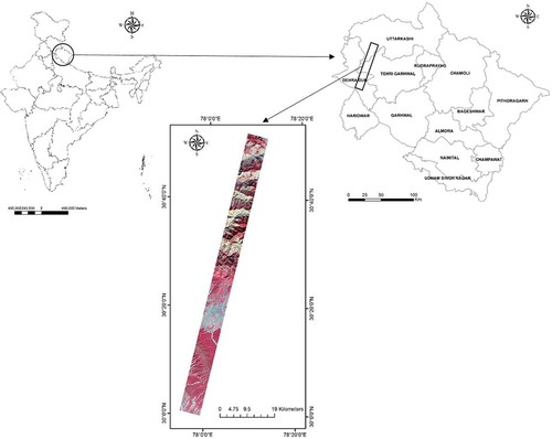
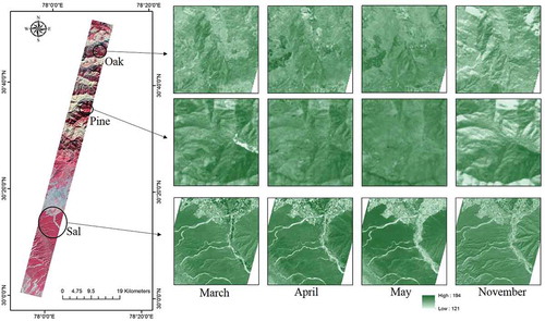
The study area extends from foothills to temperate Himalaya of Garhwal region in western Himalaya. The area is a subset of Landsat image and lies between 30°51′15.2605″N, 78°12′45.9747″E and 29°55′53.7906″N, 77°53′34.8762″E along a north-southern gradient in Garhwal Himalaya (Figure 1). Total geographical area is 70,896.69 ha. The altitudinal gradient varies from 280 to 2679 m above mean sea level (MSL). The area covers three districts of Uttarakhand, namely Dehradun, Tehri Garhwal and Uttarakashi as shown in Figure 1. The study area has two major types of forests, i.e. moist deciduous forest and Himalayan moist temperate forest (Champion & Seth, 1968). The moist deciduous forest is dominated by sal and is found in Shiwalik range of Himalaya up to 1000 m. Himalayan moist temperate forest is further classified into two broad groups based on the leaf structure which can be needle leaf moist temperate forest and broadleaf moist temperate forest. Chir pine is the dominant species in the needle leaf forest which is present between altitude ranges from 300 to 1800 m above MSL. Broadleaf moist temperate forest comprises Quercus leucotrichophora, Quercus floribunda, Rhododendron arboreum and Myrica esculenta tree species. Since these forests are mostly dominated by Quercus sp., they are called oak forests. This forest is found up to an altitude of 3000 m starting from 1200 m above MSL (Singh & Singh, 1987).

Figure 1. Study area (part of Uttarakhand in western Himalaya).

Methodology

Based on the phenological characteristics of the three different gregarious forest types, temporal satellite data were selected. Multispectral Landsat 8 Operational Land Imager (OLI) satellite data of 9 months during 2014–2015 period have been used for vegetation mapping (Table 1). All the data were atmospherically corrected using ATCOR 2014 (ATmospheric CORrection) tool compatible with Erdas Imagine 2014.

Table 1. Date of pass of Landsat 8 satellite data used for the study.

Sr. No. (band code)	Date of pass
1	13 March 2014
2	14 April 2014
3	23 October 2014
4	24 November 2014
5	10 December 2014
6	12 February 2015
7	17 April 2015
8	3 May 2015
9	19 May 2015

The path and row of the nine Landsat OLI image used for the study was 146 and 39, respectively. Different vegetation indices for these nine satellite data were calculated. To reduce the size of the temporal vegetation index, database separability analysis was carried out. This results in final temporal vegetation index database which was further used for PCM classifier. Digital elevation model (DEM) was also used as an input for the classification where it helps to separate the species at different altitude gradient. The classified map was finally proceeded for the accuracy assessment (Figure 2). Classification of the single date (November 2015) imagery was also done for comparison of the results of the multi-date NDVI database. The accuracy of both the methods was also compared.

Figure 2. Flow diagram of methodology adopted for species discrimination.

Phenology

Phenological observation provides background information on functional rhythm of organisms and communities (Singh & Singh, 1992). Phenology in general is the functional key of a plant which determines the growth and development pattern (Bronstein, Gouyon, Gliddon, Kjellberg, & Michaloud, 1990; Rathcke, 1983). This pattern is unique to a specific and helps in discrimination of one species from the other. In the present study, Shorea robusta, Pinus roxburghii and Q. leucotrichophora were considered for this phenological separability. The phenology of the species varies according to its habitat. Sal forest shows distinct phenological changes in the satellite image for different seasons. In the month of January, sal starts shedding its leaves while the peak flowering is in the month of April. In the satellite images, these changes can be observed easily. Pine and oak forests being evergreen in nature also show shedding of leaves but changes are not so distinct which is difficult to observe in the images. Leaf flushing in oak forest is observed to be at the peak during mid-April, similar to pine forest. The peak drops gradually in pine forest while in oak forest, it shows sudden drop after April and again rises in the month of October and November. Leaf flushing is not observed in pine forest in the month of October and November. The phenology of the three species has been shown in Table 2.

Table 2. Phenological activity of the three plant species (sal, pine and oak) used for spectral separation.

Species	January	February	March	April	May	June	July	August	September	October	November	December
Sal	↓	↓	↓	↑ ҈	↑ ҈ ∆	∆	§	§	–	–	–	↓
Pine	↓	↓	҈	↑ ҈	↑ ҈ ∆	∆	↑	–	§	↓	↓§	↓
Oak	–	–	↑	↑ ҈	↓ ҈	↓	§	§↑	§∆	∆↑	∆	–

Note: ↓: Leaf fall; ↑: leaf flush ; ҈: flowering; ∆: fruiting; §: herb production (Singh & Singh, 1992).

Vegetation indices and separability analysis

Satellite data enable us to observe the earth across the entire electro-magnetic spectrum at frequent intervals. The leaves reflect NIR (near infra-red) strongly which is detected by the sensors on the satellite. As the density of the leaves in the plant canopy changes from one season to another, the reflectance properties of the plant canopy also change. This information can be transformed into vegetation indices through mathematical algorithms. Different vegetation indices, viz. NDVI, SAVI, TNDVI (transformed normalized difference vegetation index), GNDVI (green NDVI), RDVI (renormalized difference vegetation index), SARVI (soil and atmospherically resistant vegetation index) and SR, were used in this study to identify the suitable index having higher seperability (Table 3). Among these vegetation indices, NDVI is the most widely used vegetation index for vegetation mapping and monitoring (Chong & Zhiyuan, 2011; Song, Xing, Liu, Liu, & Kang, 2011; Zhang, Li, Wu, & Liu, 2011). Most of indices used in the study are modified from NDVI which are GNDVI, TNDVI, RDVI and SAVI. SARVI is the index where soil and atmosphere both are taken into consideration and it uses NIR, red and blue bands. SR is the simple ratio between NIR and red region bands.

Table 3. Vegetation indices used which has been considered in the study.

S. No.	Vegetation index	Equation	Reference
1	NDVI		Rouse, Haas, Schell, Deering and Harlan (1974)
2	SAVI		Huete (1988)
3	SR		Jordan (1969)
4	GNDVI		Gitelson, Kaufman and Merzlyak (1996)
5	TNDVI		Bannari, Asalhi and Teillet (2002)
6	SARVI		Kaufman and Tanre (1992)
7	RDVI		Roujean and Breon (1995)

: Reflectance; NIR: near infrared; R: red; G: green; ; B: blue.

Different vegetation index data of different months were stacked to prepare temporal database of each vegetation index. These database were processed for separability analysis using combinations of different month data till the reasonable degree of separability was achieved. Separability can be measured using different algorithms like Euclidean distance (ED), divergence, transformed divergence, Jefferies–Matustia and Mahalanobis distance. In this study, ED measure was adopted where it uses variance and covariance statistics. If only class mean values are used, there are more chances of error/outliers, whereas computation of variance and covariance are based on squares of difference between the observed values and the class mean (Mather & Tso, 2009) has advantage over others by providing less chances of error/outliers. The algorithm used is given in the following equation:

(1)

where D is the spectral distance, i is the a particular band, N is the number of band (dimensions), is the data file value of pixel d in band i, is the data file value of pixel e in band i.

Classification and accuracy assessment approach

The geo-coded Ground truth data were collected for the identification of the locations and selection of training sets for the three forest types. Stratified random sampling was used for the ground truth data collection. These data with temporal NDVI database were used for classification of the different gregarious forest types. Fuzzy classification technique is known to be successful in categorization of complex land cover also (Okeke & Karnieli, 2006). FCM (fuzzy C-means) and PCM are two general classifiers used for image classification. In the current study, PCM is preferred over FCM as it enables to separate a particular class. PCM is the modification of FCM. It assigns to representative feature points the highest possible membership, while unrepresentative points get low membership (Krishnapuram & Keller, 1993). The objective function for PCM is given in the following equation:

(2)

For all i,

For all j,

For all i,j,

is the membership of pixel i in class j, N is the total number of pixels, m is the weighted constant , = cluster center for class j, = feature vector for pixel i, A is the weight matrix.

The supervised classification technique (Equation (2)) has been used for discrimination of the three gregarious forest types as it has a unique feature of extracting single class. This means that the membership assigned to a class in a pixel is independent of the membership assigned to other classes in the same pixel. The Cosine norm (Equation (3)) is used in the algorithm to classify a feature using the threshold value. It is a measure of similarity between two vectors of an inner product space that measures the cosine of the angle between them. The similarity in the class can be well measured by this norm as it provides more homogeneity in the output image. Cosine is useful in handling complex high dimensional data sets and achieving stable products (Tyagi & Kumar, 2015; Vanisri & Loganathan, 2011).

(3)

where is the vector pixel value and is the mean vector value of a class.

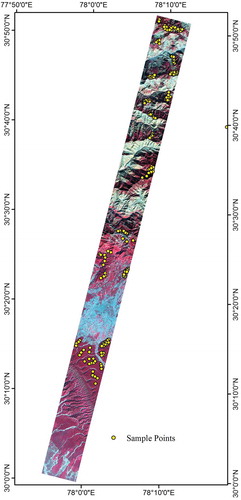
The composition of the vegetation varies with altitude, slope and aspect. Shuttle Radar Topography Mission DEM of 30 m was used where it provided information about the elevation, slope and aspect. The classified data were further improved using DEM for elevation variability. The final output product (classified image) was preceded for accuracy assessment based on randomly selected points (100 points per species) (Figure 3).

Figure 3. Distribution map of field sample points.

Results

Identification of the appropriate database

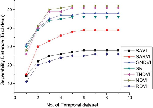
Temporal database of different vegetation indices was compared for the seperability analysis using ED. Out of seven vegetation indices, NDVI was found to have highest separation for the three species (Figure 4). RDVI had the lowest ED (26) for separation of these species. TNDVI and NDVI were found to have similar separability values, i.e. 51 and 52, respectively. All the indices showed an increasing trend up to addition of four temporal datasets beyond which it showed saturation. Since NDVI had the highest seperability, it was selected for the dimension reduction.

Figure 4. Seperability analysis of different vegetation indices using Euclidean distance.

For selection of optimum dates, ED from the combinations pairs of the selected species was used taking all the temporal datasets (Table 4). Minimum ED (separability) ranged from 28 to 52 using two to nine layers, respectively. Sal and pine had the least seperability (52) while oak and pine were found to have maximum seperability (125). For classification, minimum seperability among the species was considered which was between sal and pine. Based on the minimum separation value, four temporal images (13 March 2014, 24 November 2014, 17 April 2015 and 19 May 2015) were found to be most suitable for achieving optimal results. Using these four date combination, minimum distance was found to be 50 after which the ED saturated on addition of extra datasets.

Table 4. Separability values of three different vegetation types with different bands (dates of pass).

Bands	Sal–oak	Sal–pine	Oak–pine	Minimum separation
4, 9	28	34	62	28
4, 7, 9	45	41	85	41
1, 4, 7, 9	53	50	102	50
1, 4, 7, 8, 9	53	51	103	51
1, 3, 4, 7, 8, 9	57	52	107	52
1, 3, 4, 6, 7, 8, 9	70	52	116	52
1, 2, 3, 4, 6, 7, 8, 9	72	52	118	52
1, 2, 3, 4, 5, 6, 7, 8, 9	83	52	125	52

Note: 1: 13 March 2014; 2: 14 April 2014; 3: 23 October 2014; 4: 24 November 2014; 5: 10 December 2014; 6: 12 February 2015; 7: 17 April 2015; 8: 3 May 2015; 9: 19 May 2015.

To increase the significance of temporal NDVI database, time-series plot of NDVI database of different months was prepared (Figure 5). NDVI scatter plot shows the range of NDVI for different months (12 months) which was computed for 1 year.

Figure 5. NDVI scatter plot of three different vegetation types (sal, pine and oak) in the study area.

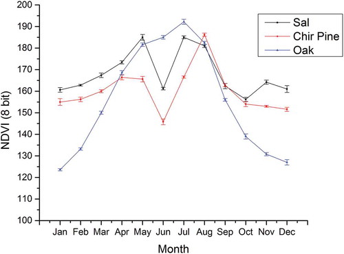
The NDVI values which were in float were converted to 8 bit unsigned data format and showed a range between 100 and 200 as required by the classifier. Different points of these species were selected and averaged to show the changes over the year. The minimum NDVI value was recorded to be 124 for oak in the month of January while it was maximum (192) for oak in the month of July. For sal, minimum NDVI was observed in the month of October (156) and maximum was in July (185). Pine forest had minimum NDVI in June (146) while maximum NDVI was in August (186). Pine showed significant increase in NDVI from June to August which is due to the onset of leaf flush during that time. Standard error (SE) was also computed for temporal NDVI of each vegetation type as shown in Figure 5. For all the three vegetation types, minimum and maximum SE was observed to be 0.37 (February) and 1.58 (December), respectively. The maximum SE was observed in the months of December and January for all the species which was 1.58 (December) for sal, 1.57 (January) for pine and 1.22 (December) for oak vegetation. Overall highest NDVI was observed in the months of July and August for all the three vegetation types due to monsoon season in selected cloud free areas. But as a result of clouds, these images could not be used for classification across the study area. Changes in the pattern of phenology were also observed from March to May where oak has shown a distinct peak in the NDVI plot as compared to pine and sal (Figure 5). In the month of November, there is change in the trend of the NDVI of sal where it is observed to increase while pine and oak still show decline in NDVI during the same period. Using the information from the seperability analysis and NDVI scatter plot of different months of the three species, temporal NDVI database was prepared. Figure 6 shows patches of three forest types and its greenness level of NDVI product at different months used in this study.

Figure 6. Temporal variation in NDVI data for different vegetation types in the study area.

Vegetation classification and accuracy assessment

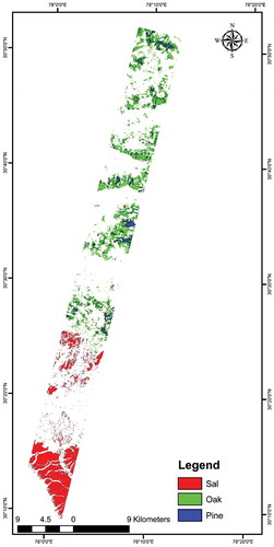
Four sets of temporal NDVI database were stacked for classification. The output classified map was generated from PCM classifier using Cosine norm. The threshold of the fuzzifier was fixed to 0.999. Sal forest occupied the southern portion of the study area which mainly covers the foothills of Himalaya. Pine and oak forests were found adjacent to sal forest. The classified map is shown in Figure 7. Total 11,729.52 ha area was classified as forest which include all three forest types. Out of these, oak forest has been found to have maximum cover (6185.34 ha). The areas of sal and pine forests were 4676.85 and 1508.49 ha, respectively.

Figure 7. Classified map of vegetation types using temporal NDVI database.

Classification of the single date multispectral data was also performed using the same classifier to assess the performance of PCM classifier on multi-date temporal database. Satellite data of 24 November 2014 was selected on the basis of seperability analysis. The accuracy of both the outputs was computed and compared.

Table 5 shows the results from accuracy assessment of the classified image from both single date and multi-date database. Total 100 samples (Congalton, 1991) were generated randomly for each class. Accuracy of these points was compared using testing samples and field data. The overall accuracy achieved was 82% and 86% using this approach for single date and multi-date data, respectively. The overall kappa accuracy for both the datasets was significant but it was higher for multi-date database (0.79) than single date (0.74) classification. The producer’s accuracy and user’s accuracy both were found to be maximum for sal forest type which was 100% and 92%, respectively, using multi-date temporal NDVI database. While for single date dataset, producer’s accuracy (92.68%) was highest for oak and user’s accuracy (88%) was highest for sal, for temporal NDVI database, the producer’s accuracy for oak forest was observed to be 88.37% and for pine forest it was 78.95%, while the user’s accuracy was observed to have opposite trend. The user’s accuracy for pine forest (90%) was observed to be more than oak forest (76%). Similar trend has been observed in the single date classification; however, multi-date classification had better accuracy.

Table 5. Result of accuracy assessment of the classified outputs using single date and multi-date.

Class name	Total classified	Reference total		Correct classified		Producer’s accuracy (%)		User’s accuracy (%)
		Single date	Multi-date	Single date	Multi-date	Single date	Multi-date	Single date	Multi-date
Sal	100	96	92	88	92	91.67	100.00	88	92.00
Pine	100	106	114	82	90	77.36	78.95	82	90.00
Oak	100	82	86	76	76	92.68	88.37	76	76.00
Total	300	284	292	246	258

Discussion

Phenology is an integral component for discriminating vegetation types using remote-sensing data. In this study, the phenological information of the three species (sal, pine and oak) was helpful in preparation of spatial vegetation map which can be used extensively in forest management activities as well as in wildlife habitat modeling (Holmgren & Persson, 2004; Immitzer, Atzberger, & Koukal, 2012; McDermid et al., 2009; Wulder, Hall, Coops, & Franklin, 2004). Accurate vegetation type map allows managers to extract information about vegetation resources at local, regional and national levels. Such mapping over a period of time can be used to monitor change in structure and composition of vegetation (Reddy & Roy, 2008).

The phenological changes of a species are helpful to discriminate it from others. Using the annual scatter plot of sal, pine and oak forests, start and end of season were identified using temporal NDVI database. Previous knowledge about phenology of these species was also used for analyzing changes. Phenological information of different seasons enable better separability than other studies which used only single date satellite data. The changes highlighted in the satellite data are due to the phenological behavior of the forest type. During the onset of the warm season, i.e. from March to May, the three species show significant differences in the phenology. During this period, there is leaf fall in sal, while pine starts flowering and leaves initiation is observed in oak (Misra, 1969; Ralhan, Khanna, Singh, & Singh, 1985). Overall signature of sal forest was observed to have more resemblance with pine forest, but use of monthly data helped in significant discrimination among the different vegetation types. As in the pre-monsoon season, oak forest showed different phenological behavior which is the critical input in discrimination of oak from the other two vegetation types. Satellite data acquired during March, April, May and November were observed as the best combination to separate out the three forest types. Upadhyay et al. (2013) have also classified moist deciduous forest in Shivaliks where multispectral satellite data of November to March period were used for the classification.

In the present study, soft classification technique has been used instead of hard classifier where pixels were classified with membership values. PCM classifier used in the study has shown better performance than other classifiers as the outputs were based on the possibility rather than probability rule. The mapping of different forest types rather than one class has been the main challenge in this approach. Most of the studies using vegetation indices and fuzzy classifier have been done for the classification of single class. This approach has been mainly used for extracting agricultural crop (Chen, Uchida, Tang, & Xu, 2004; Doraiswamy, Akhmedov, & Stern, 2006; Li, Chen, Duan, & Meng, 2010; Simonneaux & Francois, 2003; Wardlow, Egbert, & Kastens, 2007), grassland community (Oldeland, Dorigo, Lieckfeld, Lucieer, & Jürgens, 2010; Sha, Bai, Xie, Yu, & Zhang, 2008), wetland species (Adam, Mutanga, & Rugege, 2010), tropical deciduous (Krishnaswamy, Kiran, & Ganeshaiah, 2004) and coastal zone vegetation (De Lange, Van Til, & Dury, 2004). The output map from the current study classified pure forest patches of sal, pine and oak. It has been observed that pine and oak share similar habitat. In such situation, PCM classifier has helped to discriminate these two forest types successfully. This classifier can be used for both supervised and unsupervised classification. The supervised technique was preferred in the study due to availability of the sample points for species collected from ground.

The accuracy of the map is an important factor for its reliability. While using supervised classification untrained classes affects the accuracy of classification (Upadhyay, Ghosh, & Kumar, 2014), PCM classifier is not affected by these (Foody, 2000). PCM maintains high overall accuracy in classification as here 'measurement of possibility' which is used in this classifier score over the 'measurement of probability' in the classification routine. Sal forest has shown the highest individual accuracy as the chance of error of mixing with other classes was very low. Use of temporal satellite data, NDVI and fuzzy-based PCM classifier jointly has resulted in good accuracy in present study.

This approach is found to be suitable for mapping two or more vegetation types simultaneously and can also be used to monitor changes in vegetation cover over a period of time. The classifier used in this study was helpful in getting the membership values of each class and hence the contribution of two or more classes in each pixel can also be quantified. Using time-series data, PCM classifier can also be used to study the incursion of one species into another in case of invasion. The shift in the species can also be studied using this approach.

Conclusion

The discrimination and mapping of different vegetation types is challenging with the single date remote-sensing data. Present study has been carried out to distinguish sal, pine and oak forests. Fuzzy-based PCM classifier has been used to classify the vegetation. As the single date imagery was not sufficient to differentiate these three vegetation types, temporal NDVI database has been used to solve the issue. NDVI, the most commonly used vegetation index, has been used to capture the vegetation property. The phenological information of the different forest types played an important role in identifying the suitable seasons while spectral separability significantly reduced the data size and identified the bands best suited for separation of the vegetation. The accuracy of the classified map was found to be 86% which is significantly higher than the conventional classifiers (Zhang, Shi, & Liu, 2012).

Disclosure statement

No potential conflict of interest was reported by the authors.

References

- Adam, E., Mutanga, O., & Rugege, D. (2010). Multispectral and hyperspectral remote sensing for identification and mapping of wetland vegetation: A review. Wetlands Ecology and Management, 18(3), 281–296. doi:10.1007/s11273-009-9169-z
- Avci, M., & Akyurek, Z. (2004, July 12–23). A hierarchical classification of landsat TM imagery for landcover mapping. In O. Altan (Ed.) The international archives of the photogrammetry, remote sensing and spatial information sciences (Vols. XXXV-B4, pp. 511–516). Istanbul, Turkey. ISPRS.
- Bannari, A., Asalhi, H., & Teillet, P.M. (2002). Transformed difference vegetation index (TDVI) for vegetation cover mapping. In Geoscience and Remote Sensing Symposium, 2002. IGARSS’02. 2002 IEEE International (Vol. 5, pp. 3053–3055). IEEE.
- Berberoğlu, S., & Satir, O. (2008). Fuzzy classification of mediterranean type forest using envisat meris data. International Archives of the Photogrammetry, Remote Sensing and Spatial Information Sciences (ISPRS 2008), 37, 1109–1119.
- Bronstein, J.L., Gouyon, P.H., Gliddon, C., Kjellberg, F., & Michaloud, G. (1990). The ecological consequences of flowering asynchrony in monoecious fogs: A simulation study. Ecology, 71, 2145–2156. doi:10.2307/1938628
- Burrough, P.A., Wilson, J.P., Van Gaans, P.F., & Hansen, A.J. (2001). Fuzzy k-means classification of topo-climatic data as an aid to forest mapping in the greater yellowstone area, USA. Landscape Ecology, 16(6), 523–546. doi:10.1023/A:1013167712622
- Champion, H.G., & Seth, S.K. (1968). A revised survey of the forest types of India. Govt. of India Press Delhi India.
- Chen, Z., Uchida, S., Tang, H., & Xu, B. (2004). NDVI-based winter wheat unmixing for accurate acreage estimation. Geoscience and Remote Sensing Symposium, IGARSS’04. Proceedings. 2004 IEEE International Vol. 6, pp. 3977–3980.
- Chong, Z., & Zhiyuan, R. (2011). Temporal and spatial differences and its trends in vegetation cover change over the Loess Plateau. Resources Science, 33(11), 2143–2149.
- Congalton, R.G. (1991). A review of assessing the accuracy of classifications of remotely sensed data. Remote Sensing of Environment, 37(1), 35–46. doi:10.1016/0034-4257(91)90048-B
- De Lange, R., Van Til, M., & Dury, S. (2004). The use of hyperspectral data in coastal zone vegetation monitoring. EARSeL eProceedings, 3(2), 143–153.
- Doraiswamy, P.C., Akhmedov, B., & Stern, A.J. (2006). Improved techniques for crop classification using MODIS imagery. In Geoscience and Remote Sensing Symposium, 2006. IGARSS 2006. IEEE International Conference pp. 2084–2087.
- Dwivedi, R.S., & Ravisankar, T. (1991). Monitoring shifting cultivation using space-borne multlspectral and multi temporal data. International Journal of Remote Sensing, 12(3), 427–433. doi:10.1080/01431169108929663
- Foody, G.M. (2000). Estimation of sub-pixel land cover composition in the presence of untrained classes. Computers & Geosciences, 26(4), 469–478. doi:10.1016/S0098-3004(99)00125-9
- Gitelson, A.A., Kaufman, Y.J., & Merzlyak, M.N. (1996). Use of a green channel in remote sensing of global vegetation from EOS-MODIS. Remote Sensing of Environment, 58, 289–298. doi:10.1016/S0034-4257(96)00072-7
- Hasmadi, I., Mohd Zaki, H., Ismail Aa Dnan, A.M., Pakhriazad, H.Z., & Muhammad Fadlli, A.Y. (2010). Determining and mapping of vegetation using GIS and phytosociological approach in mount tahan, Malaysia. Journal of Agricultural Science, 2(2), 80–89.
- He, C., Zhang, Q., Li, Y., Li, X., & Shi, P. (2005). Zoning grassland protection area using remote sensing and cellular automata modeling—A case study in Xilingol steppe grassland in northern China. Journal of Arid Environments, 63(8), 14–26. doi:10.1016/j.jaridenv.2005.03.028
- Hilker, T., Wulder, M.A., Coops, N.C., Linke, J., McDermid, G., Masek, J.G., … White, J.C. (2009). A new data fusion model for high spatial- and temporal-resolution mapping of forest disturbance based on Landsat and MODIS. Remote Sensing of Environment, 113, 1613–1627. doi:10.1016/j.rse.2009.03.007
- Holmgren, J., & Persson, Å. (2004). Identifying species of individual trees using airborne laser scanner. Remote Sensing of Environment, 90(4), 415–423. doi:10.1016/S0034-4257(03)00140-8
- Huete, A. (1988). A Soil-Adjusted Vegetation Index (SAVI). Remote Sensing of Environment, 25(1988), 295–309. doi:10.1016/0034-4257(88)90106-X
- Immitzer, M., Atzberger, C., & Koukal, T. (2012). Tree species classification with random forest using very high spatial resolution 8-band WorldView-2 satellite data. Remote Sensing, 4(9), 2661–2693. doi:10.3390/rs4092661
- Jordan, C.F. (1969). Derivation of leaf area index from quality of light on the forest floor. Ecology, 50, 663–666. doi:10.2307/1936256
- Kaufman, Y.J., & Tanre, D. (1992). Atmospherically resistant vegetation index (ARVI) for EOS-MODIS. IEEE Transactions on Geoscience and Remote Sensing, 30(2), 261–270. doi:10.1109/36.134076
- Krishnapuram, R., & Keller, J.M. (1993). A possibilistic approach to clustering. Fuzzy Systems, IEEE Transactions On, 1(2), 98–110. doi:10.1109/91.227387
- Krishnaswamy, J., Kiran, M.C., & Ganeshaiah, K.N. (2004). Tree model based eco-climatic vegetation classification and fuzzy mapping in diverse tropical deciduous ecosystems using multi-season NDVI. International Journal of Remote Sensing, 25(6), 1185–1205. doi:10.1080/0143116031000149989
- Kumar, G.R.P., Hemanjali, A.M., Ravikumar, P., Somashekar, R.K., & Nagaraja, B.C. (2014). Assessmentof forest encroachment at belgaum district of western ghats of Karnataka using remote sensing and GIS. Journal of Environmental Biology, 35, 259–264.
- Kushwaha, S.P.S. (1991). Remote Sensing of shifting cultivation in North-Eastern India. In P. Shunjl MuraL (Ed.), Appllcation of remote sensing in Asia and oceanic-environmental change monitoring (pp. 5O·n). Tokyo: Asian association of Remote Sensing.
- Lane, C.R., Liu, H., Autrey, B.C., Anenkhonov, O.A., Chepinoga, V.V., & Wu, Q. (2014). Improved Wetland classification using eight-band high resolution satellite imagery and a hybrid approach. Remote Sensing, 6, 12187–12216. doi:10.3390/rs61212187
- Langley, S.K., Cheshire, H.M., & Humes, K.S. (2001). A comparison of single date and multitemporal satellite image classifications in a semi-arid grassland. Journal of Arid Environments, 49, 401–411. doi:10.1006/jare.2000.0771
- Li, Y., Chen, X., Duan, H., & Meng, L. (2010). An improved multi-temporal masking classification method for winter wheat identification. In Audio Language and Image Processing (ICALIP), International Conference on IEEEpp. 1648–1651.
- Lo, C.P., & Choi, J. (2004). A hybrid approach to urban land use/cover mapping using Landsat 7 Enhanced Thematic Mapper Plus (ETM+) images. International Journal of Remote Sensing, 25, 2687–2700. doi:10.1080/01431160310001618428
- Mather, P., & Tso, B. (2009). Classification methods for remotely sensed data (pp. 221–252). Boca Raton: CRC press.
- McDermid, G.J., Hall, R.J., Sanchez-Azofeifa, G.A., Franklin, S.E., Stenhouse, G.B., Kobliuk, T., & LeDrew, E.F. (2009). Remote sensing and forest inventory for wildlife habitat assessment. Forest Ecology and Management, 257(11), 2262–2269. doi:10.1016/j.foreco.2009.03.005
- Millward, A.A., Piwowar, J.M., & Howarth, P.J. (2006). Time series analysis of medium-resolution, multisensor satellite data for identifying landscape change. Photogrammetric Engineering and Remote Sensing, 72(6), 653–663. doi:10.14358/PERS.72.6.653
- Misra, G., Kumar, A., Patel, N.R., & Zurita-Milla, R. (2014). Mapping a specific crop—a temporal approach for sugarcane ratoon. Journal of the Indian Society of Remote Sensing, 42(2), 325–334. doi:10.1007/s12524-012-0252-1
- Misra, R. (1969). Studies on the primary productivity of terrestrial communities at Varanasi. Tropical Ecology, 10, 1–15.
- Morton, D.C., De Fries, R.S., Nagol, J., Souza, C.M., Kasisch, E.S., Hurt, G.C., & Dubahaya, R. (2011). Mapping canopy damage from understory fires in Amazon forests using annual time series of Landsat and MODIS data. Remote Sensing of Environment, 115, 1706–1720. doi:10.1016/j.rse.2011.03.002
- Musande, V., Kumar, A., & Kale, K. (2012). Cotton crop discrimination using fuzzy classification approach. Journal of the Indian Society of Remote Sensing. doi:10.1007/s12524-012-0201-z
- Okeke, F., & Karnieli, A. (2006). Methods for fuzzy classification and accuracy assessment of historical aerial photographs for vegetation change analyses. Part I: Algorithm development. International Journal of Remote Sensing, 27(1), 153–176. doi:10.1080/01431160500166540
- Oldeland, J., Dorigo, W., Lieckfeld, L., Lucieer, A., & Jürgens, N. (2010). Combining vegetation indices, constrained ordination and fuzzy classification for mapping semi-natural vegetation units from hyperspectral imagery. Remote Sensing of Environment, 114(6), 1155–1166. doi:10.1016/j.rse.2010.01.003
- Pettorelli, N., Laurance, W.F., O’Brien, T.G., Wegmann, M., Nagendra, H., & Turner, W. (2014). Satellite remote sensing for applied ecologists: Opportunities and challenges. Journal of Applied Ecology, 51(4), 839–848. doi:10.1111/1365-2664.12261
- Powell, S.L., Cohen, W.B., Sean, P., Healey, S.P., Kennedy, R.E., Moisen, G.G., … Ohmann, J.L. (2010). Quantification of live aboveground forest biomass dynamics with landsat time series and field inventory data: A comparison of empirical modeling approaches. Remote Sensing of Environment, 114, 1053–1068. doi:10.1016/j.rse.2009.12.018
- Ralhan, P.K., Khanna, R.K., Singh, S.P., & Singh, J.S. (1985). Phenological characteristics of the tree layer of Kumaun Himalayan forests. Vegetatio, 60(2), 91–101. doi:10.1007/BF00040351
- Rathcke, B.J. (1983). Competition and facilitation among plants for pollination. In L. Real (Ed.) Pollination biology. 305–338 Academic Press INC New York.
- Reddy, C.S., & Roy, A. (2008). Assessment of three decade vegetation dynamics in mangroves of Godavari delta, India using multi-temporal satellite data and GIS. Research Journal of Environmental Sciences, 2(2), 108–115. doi:10.3923/rjes.2008.108.115
- Roujean, J.L., & Breon, F.M. (1995). Estimating PAR absorbed by vegetation from bidirectional reflectance measurements. Remote Sensing of Environment, 51(3), 375–384. doi:10.1016/0034-4257(94)00114-3
- Rouse, J.W., Haas, R.H., Schell, J.A., Deering, D.W., & Harlan, J.C. (1974).Monitoring the vernal advancements and retrogradation (Greenwave Effect) of nature vegetation; NASA/GSFC Final Report; NASA: Greenbelt, MD, USA.
- Roy, P.S., Behera, M.D., Murthy, M.S.R., Roy, A., Singh, S., Kushwaha, S.P.S., & Gupta, S. (2015). New vegetation type map of India prepared using satellite remote sensing: Comparison with global vegetation maps and utilities. International Journal of Applied Earth Observation and Geoinformation, 39, 142–159. doi:10.1016/j.jag.2015.03.003
- Rusanen, J., Muilu, T., Colpaert, A., & Naukkarinen, A. (2001). Finnish socio-economic grid data, GIS and the hidden geography of unemployment. Tijdschrift Voor Economische En Sociale Geografie, 92(2), 139–147. doi:10.1111/1467-9663.00146
- Sha, Z., Bai, Y., Xie, Y., Yu, M., & Zhang, L. (2008). Using a hybrid fuzzy classifier (HFC) to map typical grassland vegetation in Xilin River Basin, Inner Mongolia, China. International Journal of Remote Sensing, 29(8), 2317–2337. doi:10.1080/01431160701408436
- Simonneaux, V., & Francois, P. (2003). Identifying main crop classes in an irrigated area using high resolution image time series. In Geoscience and Remote Sensing Symposium, 2003. IGARSS’03. Proceedings. 2003 IEEE International Vol. 1, pp. 252–254.
- Singh, J.S., & Singh, S.P. (1987). Forest vegetation of the Himalaya. The Botanical Review, 53(1), 80–192. doi:10.1007/BF02858183
- Singh, J.S., & Singh, S.P. (1992). Forests of himalaya structure, functioning and impact of man. Gyanodaya prakashan, Nainital, India.
- Song, F.Q., Xing, K.X., Liu, Y., Liu, Z.C., & Kang, M.Y. (2011). Monitoring and assessment of vegetation variation in northern Shaanxi based on MODIS/NDVI. Acta Ecologica Sinica, 31(2), 354–363.
- Tingting, L., & Chuang, L. (2010). Study on extraction of crop information using time-series MODIS data in the Chao Phraya Basin of Thailand. Advances in Space Research, 45(6), 775–784. doi:10.1016/j.asr.2009.11.013
- Tyagi, U., & Kumar, A. (2015). Similarity and dissimilarity measures with fuzzy classifiers: SMIC tool. Journal of Basic and Applied Engineering Research, 2(16), 1411–1416.
- Upadhyay, P., Ghosh, S.K., & Kumar, A. (2014). A brief review of fuzzy soft classification and assessment of accuracy methods for identification of single land cover. Studies in Surveying and Mapping Science (SSMS), Vol. 2, 1-13.
- Upadhyay, P., Kumar, A., & Ghosh, S.K. (2013). Fuzzy based approach for moist deciduous forest identification using MODIS temporal data. Journal of the Indian Society of Remote Sensing, 41(4), 777–786. doi:10.1007/s12524-013-0267-2
- Vanisri, D., & Loganathan, C. (2011). An efficient fuzzy possibilistic C-Means with penalized and compensated constraints. Global Journal of Computer Science and Technology, 11(3), 15–21.
- Wardlow, B.D., & Egbert, S.L. (2008). Large-area crop mapping using time-series MODIS 250 m NDVI data: an assessment for the U.S. central great plains. Remote Sensing of Environment, 112, 1096–1116. doi:10.1016/j.rse.2007.07.019
- Wardlow, B.D., Egbert, S.L., & Kastens, J.H. (2007). Analysis of time-series MODIS 250 m vegetation index data for crop classification in the US central great plains. Remote Sensing of Environment, 108(3), 290–310. doi:10.1016/j.rse.2006.11.021
- Wulder, M.A., Hall, R.J., Coops, N.C., & Franklin, S.E. (2004). High spatial resolution remotely sensed data for ecosystem characterization. BioScience, 54(6), 511–521. doi:10.1641/0006-3568(2004)054[0511:HSRRSD]2.0.CO;2
- Xiao, X.M., Zhang, Q., & Braswell, B. (2004). Modeling gross primary production of temperate deciduous broadleaf forest using satellite images and climate data. Remote Sensing of Environment, 91(256), 70th ser. doi:10.1016/j.rse.2004.03.010
- Xie, Y., Sha, Z., & Yu, M. (2008). Remote sensing imagery in vegetation mapping: A review. Journal of Plant Ecology, 1(1), 9–23. doi:10.1093/jpe/rtm005
- Zhang, H., Shi, W., & Liu, K. (2012). Fuzzy-topology-integrated support vector machine for remotely sensed image classification. IEEE Transactions on Geoscience and Remote Sensing, 50(3), 850–862. doi:10.1109/TGRS.2011.2163518
- Zhang, L.Z., Li, M., Wu, Z.F., & Liu, Y.J. (2011). Vegetation cover change and its mechanism in Northeast China based on SPOT/NDVI data. Journal of Arid Land Resources and Environment, 25(1), 171–175.