Mapping ultramafic complexes using airborne imaging spectroscopy and spaceborne data in Arctic regions with abundant lichen cover, a case study from the Niaqornarssuit complex in South West Greenland

ABSTRACT

This study investigates the usage of HyMAP airborne hyperspectral and Sentinel-2, ASTER and Landsat-8 OLI spaceborne multispectral data for detailed mapping of mineral resources in the Arctic. The EnMAP Geological Mapper (EnGeoMAP) and Iterative Spectral Mixture Analysis (ISMA) approaches are tested for mapping of mafic-ultramafic rocks in areas covered by abundant lichen. Using the Structural Similarity Index Measure (SSIM), the output classification results from airborne data are quantitatively compared to the available geological map and to the HyMAP reference data in case of using spaceborne dataset. Results demonstrate the capability of both airborne and spaceborne data to provide large-scale reconnaissance mapping of geologic materials over vast arctic regions where field access is limited. The distributions of three ultramafic units (dunite, peridotite, pyroxenite) and one mafic unit (gabbro) are mapped based on analyzing specific visible and near-infrared and short-wave-infrared spectral features. The extent of peridotite and dunite units mapped using both approaches is consistent with geological map, whereas pyroxenite abundance maps show different patterns in their distribution as compared to the geological map. The results suggest that EnGeoMAP method has a better performance than ISMA method for mapping the dunite unit, whilst ISMA performs better for mapping peridotite and pyroxenite rocks.

KEYWORDS:

• Spectroscopy
• mineral mapping
• lichen
• unmixing
• ultramafic
• arctic
• non-invasive

Introduction

Non-invasive remote sensing is a suitable exploration technique to cover large areas with reduced financial input, if compared to classical approaches. Considerable research has been devoted to the use of multi- and hyperspectral remote sensing technology for geological applications in arid and semi-arid environments (Buckley et al., 2013; Gao et al., 2017; Harris et al., 2005; Huo et al., 2014; Kopačková & Koucká, 2017; Marion & Carrère, 2018; Notesco et al., 2016); however, less research has been devoted to the efficacy of these methods for mineral exploration purposes in the Arctic, and therefore, this is still an open field for research.

The remote nature and the challenges posed by the Arctic environment reduce the capacity of traditional techniques to economically explore and locate mineral resources. Greenland for example, is an ideal study area for the application of remote sensing techniques (Bedini, 2009, 2011; 2012; Budkewitsch et al., 2000; Salehi, 2018). Large parts of Greenland, that are known for excellent potentials for natural resources, including zinc, lead, gold, copper, iron ore, and heavy and light rare earth elements, are largely underexplored due to the obstacles created by topography, remoteness and harsh climate conditions. It is, therefore, very important to aim for good spatial coverage of the regions of interest and areas under investigation by applying efficient data acquisition techniques. Different remote sensing techniques for geologic mapping and mineral exploration have been studied, developed and applied in areas of difficult access in Greenland (Salehi, 2018). Satellite remote sensing has been mainly used for delineating the lithological units and providing key information for early mineral exploration. Wide-swath spaceborne sensors such as Landsat-8 OLI, ASTER, and Sentinel-2 enable the repetitive coverage of large regions with low/medium spatial and spectral resolutions at no additional data costs for potential exploration clients (Salehi et al., 2019a). On the other hand, narrow-swath commercial sensors such as Worldview-3 are more suited for a detailed mapping program at exploration tenement level, due to their higher spatial and spectral resolutions (Kruse & Perry, 2013). Such data lack the spatial capacity and the financial viability for greenfield reconnaissance explorations over larger areas and may be deferred to later project stages. In addition to the spaceborne data, airborne imaging systems have been successfully used for regional mapping of rock types and mineral prospecting in Greenland over the last two decades (Bedini, 2009, 2012; Salehi & Thaarup, 2018; Tukiainen & Thomassen, 2010; Tukiainen & Thorning, 2005). The disadvantages of airborne imaging systems are low coverage area and that these data are produced at substantially high costs per unit area of ground coverage compared to the rapidly growing fleet of multispectral, and future full range hyperspectral spaceborne imaging systems with an open data policy. Therefore, it is not cost-effective to map a large area using an airborne system. Other approaches such as off-nadir helicopter-based (Salehi et al., 2019b), ship-based (Salehi et al., 2018; Salehi & Thaarup, 2018) and long-range terrestrial outcrop sensing (Lorenz et al., 2018; Rosa et al., 2017; Salehi & Thaarup, 2018) have been recently established to expand the scale of mapping in Arctic regions in a time- and cost-effective manner as geophysical data suppliers in the later stage of an exploration project, after regions of exploration interest have been identified from spaceborne data. Using such scanning setups, steep cliff sections and quarry walls can be scanned with a more appropriate viewing direction and a higher image resolution than can be detained from airborne and spaceborne platforms (Salehi, 2018).

Another important factor in using remote sensing technology for mineral exploration is the selection of the most optimal approaches for mapping based on environmental conditions. One limitation of current state-of-the-art methods is the sub-pixel spectral mixture of lichens and rocks that can have an adverse effect on identifying rocks and minerals using imaging sensor systems (Salehi et al., 2017b). Since the nineties, there have been a number of studies that have investigated the potential of using airborne and simulated spaceborne hyperspectral data for discrimination of mafic and ultramafic rocks in the Canadian north, where rocks are exposed in presence of lichens (Harris et al., 2005; Rogge et al., 2014b). These studies have concluded that Spectral Mixture Analysis techniques are useful means of reducing the mixed pixel problem and acquiring sub-pixel scale information. However, to our knowledge, no research has been done on investigating the potential of multispectral spaceborne datasets for geological mapping applications in areas with abundant lichens. The problem of spectral mixing is aggravated by coarser spatial resolution of these sensors; nevertheless, they represent the most cost-effective approach to extract geological information, provided that suitable mapping techniques or indicators to target specific mineral deposit types are used.

The research presented in this article is primarily focused on the mapping of ultramafic rocks, as they are an important host rock for nickel, platinum group elements (PGE) and chromium, minerals that have been identified as critical elements for the development of new green technologies. The study carried out by Mielke et al. (2014) shows some examples for mapping PGE related mine waste near Rustenburg South Africa, focussing especially on the visible and near-infrared (VNIR) for the characterization of mafic and ultramafic mine waste material. This approach has not been tested in an Arctic environment, neither has it been used for the direct exploration of ultramafic complexes, giving a direct link to the geological map of the area. On the other hand, successful mapping studies in Canada have been limited to hydrated minerals (Harris et al., 2005; Rogge et al., 2014b). Rogge et al. (2014b) have focused on few short-wave-infrared (SWIR) spectral features associated with antigorite (2285, 2325 nm), actinolite (2245, 2315, 2386 nm) and clinochlore (2345) minerals to discriminate the mafic and ultramafic rock units. According to Rogge et al. (2014b), ferrous (Fe⁺²) and ferric (Fe⁺³) features within the VNIR spectral range are heavily suppressed by the various lichen species in their study area and therefore the VNIR bands were deployed to map non-geological materials rather than differentiating mafic and ultramafic rocks.

Given the limitations discussed earlier in the text, the objectives of this study are to: (1) evaluate the potential of airborne hyperspectral imagery and spaceborne multispectral data for producing lithological–compositional maps under Arctic conditions and in areas with abundant lichens; (2) expand the possible use of spectroscopy for discrimination of mafic-ultramafic rock types by considering both primary (olivine, pyroxene) and secondary (amphibole) mineralogy; and (3) evaluate the performance of two unmixing approaches for mapping different mafic-ultramafic bodies potentially associated with PGE and/or Ni-sulfide mineralisation.

The results of this study should have considerable potential to evaluate the use of hyperspectral and multispectral remote sensing for geological purposes in the Arctic regions.

Materials and methods

Sentinel-2, ASTER and Landsat-8 OLI data are evaluated as a first-order tool to obtain reconnaissance level information from the study area in South West Greenland. The analysis of airborne HyMap imagery is carried out to obtain detailed complementary lithological–compositional maps.

The performance of two mapping approaches: the Iterative Spectral Mixture Analysis (ISMA) (Rogge et al., 2006) and the EnMAP Geological Mapper (EnGeoMAP) (Mielke et al., 2016; Rogass et al., 2014) is investigated for mapping the distribution of mafic-ultramafic units. These two approaches represent interesting candidates for a comparison of two different purely data-driven unmixing approaches. To enhance comparability, the same set of endmembers was used for ISMA and EnGeoMAP generated from Spatial–Spectral Endmember Extraction (SSEE) approach (Rogge et al., 2012, 2007). In addition, band selection is used for optimizing the spectral unmixing. This is achieved by applying a knowledge – driven band selection routine, as in case of ISMA; and a purely data – driven band selection technique as in case of EnGeoMAP.

X-ray fluorescence (PANalytical AXIOS Advanced RFA) and in situ and laboratory spectral measurements of representative samples are carried out to describe mineralogical composition and spectral characteristics of the mafic-ultramafic rocks. In addition, the report published by 21^st North exploration company provides insights to the mineralogical composition of the samples, which are largely dominated by olivine (dunites) and pyroxene (pyroxenites) (Simard et al., 2014). The accuracy of the final mapping products is validated by a direct comparison of the results to the ultramafic units of the geological map for the airborne data and to the HyMAP reference image for the spaceborne dataset and by using the Structural Similarity Measure method (Wang et al., 2004).

Study area

The southern part of the Palaeoproterozoic Nagssugtoqidian orogen (SNO) in West Greenland is dominated by tonalitic to granodioritic reworked Achaean orthogneisses interleaved with sulphide-graphite rich belts of Paleoproterozoic supracrustal and anorthositic-ultrabasic intrusive rocks occurring within E-W trending high-strain zones (Figure 1). The region is mostly known for hosting an important alkaline intrusive event that includes the Sarfartoq carbonatite complex and an associated swarm of mostly contemporaneous lamprophyre and diamond-bearing kimberlite dykes (Jensen et al., 2002; Larsen & Rex, 1992; Secher & Larsen, 1980).

Figure 1. General 1:500 000 geological map across the southern Nagssugtoqidian Orogen simplified from Garde and Marker (2010). The location of number of mafic and ultramafic complexes mapped by processing of regional HyMAP data are shown in pink ovals. The Niaqornarssuit complex is highlighted by a black oval

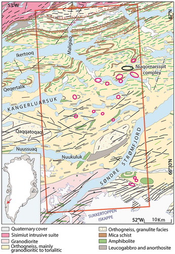
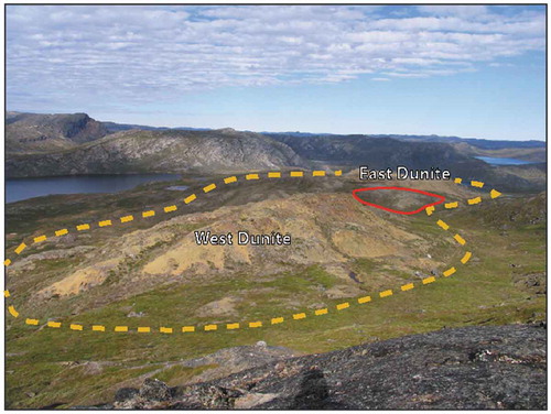
In addition, several mafic-ultramafic bodies/intrusions/complexes hosted in Archean gneisses and composed of massive dunite, peridotite, and pyroxenite have been identified over the past years within the SNO. The Niaqornarssuit complex is the best known of the ultramafic complexes within this region, which was briefly visited by Kryolitselskabet Øresund (KØ) Company in 1977. The complex is located at approximately 8 km east of the ice-free Sarfannguit Fjord and 65 km southwest of Kangerlussuaq and at an altitude of approximately 400 m (see black oval in Figure 1). It was described as an 1 × 3 km elliptical massif of E-W oriented ultramafic rocks composed of homogeneous dunite with a relatively thin zone of gabbro along with the contact (Gothenborg & Keto, 1980). The area terrane is characterized with moderate relief hills, commonly without any significant vegetation except in low-lying, south-facing slopes and depressions where shrubs may reach 1–2 m of height. Rock encrusting lichens are predominant on bedrock surfaces and cover from 0% to 90% of exposed surfaces depending on rock type (Figure 2). This complicates the remote sensing-based mapping of mafic to ultramafic rock units in the region.

Figure 2. View of the Niaqornarssuit complex, highlighting characteristic features of the study area terrane (e.g. variability in spatial continuity of exposed outcrop, lichen coatings, and low-lying vegetation cover)

In 2010, following on KØ’s work on the Niaqornarssuit complex, 21^st North Exploration Company proceeded with a nine-day field reconnaissance program. Around 160 samples were collected from the dunitic intrusions (Figure 3) and were further analysed to obtain whole-rock geochemical data. A much more detailed description of the complex combined with a 1:10 000 geological map was produced by the company in the same year.

Figure 3. True color HyMAP image and detailed geological map of the Niaqornarssuit complex produced by 21^st North Exploration Company. Yellow dots show the locations of surface samples that have been collected for reconnaissance work and mapping over the area. Samples that are selected for XRF and ASD analysis are indicated by red color

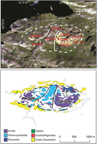
The exploration work carried out by the 21^st North Exploration Company suggests that the complex is dominated by two main dunite bodies characterized by yellowish-green weathered outcrops: The West dunite and the East dunite (Figure 3). According to a confidential report presented by the company (Simard et al., 2014), a rough outline of the stratigraphy comprises the following rock units: (1) a chilled margin at the basal level of the intrusion mostly of peridotitic composition, directly overlying basement gneisses and granites at the contact, (2) magnetite and chromite-rich, homogeneous and medium-grained dunite grading into more pure dunite (the dunite hosts numerous peridotite-pyroxenite layers and dykes and small mineralized gossans are locally present in the southeastern part of the dunite), (3) peridotite composed of olivine-peridotite at the bottom and more evolved pyroxene-rich peridotite at upper levels, (4) coarse-grained to pegmatitic pyroxenite forming a massive and homogeneous unit in the northeastern part of the complex, and (5) a discontinuous layer of medium-grained and banded metagabbro or hornblende-gneiss interleaved with, and possibly intruding into, the upper part of the pyroxenite. Surface mineralization in the Niaqornarssuit complex is almost entirely restricted to small rusty beds in the East dunite where it forms discontinuous and strongly weathered gossans (Simard et al., 2014). The size of such zones is rarely more than 10 m long and 0.3 to 0.5 meters wide. The rusty lenses are mostly hosted by peridotite/pyroxenite layers and veins within the dunite, suggesting remobilization of a primary sulphide source into narrow zones at surface. Due to the weathered nature of these zones, fresh sulphide mineralization is often not observed at surface but rather consists of (a) strongly rusted malachite-stained gossan boulders, and (b) small conspicuous ridges partly buried in the sandy slopes of the dunite (Simard et al., 2014). The sulphide paragenesis consists of pentlandite, pyrrhotite and chalcopyrite (Simard et al., 2014).

Regional airborne hyperspectral data

A regional airborne hyperspectral dataset was acquired using a HyMap sensor (Cocks et al., 1998) in 2002, covering an area of approximately 7500 km² between Sisimiut and Kangerlussuaq (Søndre Strømfjord) in South West Greenland (Tukiainen & Thorning, 2005). Due to the rugged terrain of the survey area, the ground spatial resolution varies from 3 to 5 m depending on the altitude from the surveyed ground. The sensor has 126 channels over the 0.45–2.5 µm wavelength range with average spectral resolution of ~10 nm.

The aim of the survey was to investigate the potential of airborne hyperspectral dataset for finding diamond-bearing kimberlite dykes (Tukiainen & Thorning, 2005). Further processing and interpretation of HyMap data revealed a number of mafic and ultramafic complexes (Salehi & Thaarup, 2018) (see pink ovals in Figure 1). One such complex occurs to the east of the head of the fjord Kangerluarsuk, a feature confirmed by field work in 2016 (Salehi & Thaarup, 2018). A portion of this survey data (~3.5 X 2.5 km² region) coincides with the Niaqornarssuit complex.

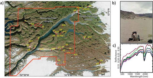
The data were geometrically corrected and geocoded by Tukiainen and Krebs (2004) using the PARGE (Parametric Geocoding) software (Schläpfer & Richter, 2002). This procedure reconstructs the scanning geometry for each image pixel using position, attitude, and terrain elevation data. The geocoded radiance data were converted to at-surface reflectance values using Atmospheric and Topographic Correction for airborne imagery (ATCOR-4) program in rugged terrain mode (Salehi, 2018; Tukiainen & Krebs, 2004). A detailed digital elevation model for the entire survey area produced at the Geological Survey of Denmark and Greenland’s photogrammetric laboratory was used in this step. The rural model was chosen, 3000 m above sea level with water vapour column of 2.0 gcm⁻² from sea level to space. Maritime aerosol type or mixed rural/maritime options may give better results for the coastal areas. Furthermore, higher values for the water vapour column may be justified for the areas adjacent to and/or dissected by fiords. At-surface reflectance values from the ATCOR-4 processing were adjusted by an empirical line approach using ground-based reflectance measurements from calibration sites measured with an Analytical Spectral Devices FieldSpec®3 HiRes Spectroradiometer (ASD). ASD data were collected during the hyperspectral scanner overflights from numerous pseudo-invariant features (PIFs) that were mainly homogenous, vegetation and lichen-free exposures of alluvial material (Tukiainen & Krebs, 2004; Tukiainen et al., 2003) (Figure 4(a)). Reflectance measurements for one PIF locality are shown in Figure 4(c). The locality is a part of a major flat area composed of silt deposited in an ice-dammed lake (Figure 4(b)) and is measured both in sunlight and using a tungsten-halogen lamp (Tukiainen et al., 2003).

Figure 4. (a) Field localities where spectroradiometric measurements were carried out. The area covered by the airborne hyperspectral survey is indicated by the red line. K = kimberlitic rocks, L = lamproitic rocks, LG = local geology, S = rocks of the Sarfartoq carbonatite complex, P = pseudo-invariant fields, Plant = vegetation; (b) locality P3 on the silt formation in the vicinity of Kangerlussuaq airport; (c) individual measurements from the locality P3

Remaining albedo differences due to imperfect foregoing atmospheric correction and global bidirectional reflectance distribution function (BRDF) suppression can still lead to sinusoidal perceptible albedo differences between the data takes (Figure 5). To reduce these remaining data trends, the detrending approach was applied that helped to significantly suppress those trends (Figure 5). It was assumed that data trends, which do not reflect surface reflectance distribution, might bias succeeding data analysis such as spatio-spectral classification and segmentation. Other approaches were not tested but might be also applicable.

Figure 5. Airborne HyMAP data before and after removal of remaining albedo differences using detrending approach

Of the 126 atmospherically corrected channels of HyMAP data, 106 channels over the 0.47- to 2.46-μm spectral range were selected for further analysis. Channels not used are associated with the large water vapor absorption features near 1.4 and 1.9 μm. The images were mosaicked using ENVI (ENvironment for Visualizing Images; Harris Geospatial Solutions, Broomfield, Colorado). To improve the quality of the mosaic image, each flight line was subject to masking for clouds, cloud shadows, water, snow\ice and areas of poorly illuminated steep terrain (steep slopes facing away from the incident solar radiation). Water, snow\ice and low albedo pixels show lower reflectance values within the short-wave-infrared range as compared to rock outcrops. The mean reflectance value was calculated for all the pixels of each flight line throughout the SWIR range (1.5–2.46 μm) and a single band image (here referred to as mean reflectance image) was generated. Based on the statistics of the mean reflectance at wavelengths 1.5–2.46 μm, a threshold was set to mask out pixels related to water, snow\ice and cast shadow. A pixel containing cloud or cloud shadow was determined by comparing reflectance levels for five channels (corresponding to wavelength positions 0.5, 1.01, 1.23, 1.54, and 2.11 μm) against threshold values. Bright pixels were flagged as cloud contaminated and dark pixels were flagged as cast shadow. The two aforementioned masks were then combined into a single mask for each flight line.

ASD and fluorescence spectroscopy

Of 160 samples collected by 21^st North exploration company, 18 were processed for X-ray fluorescence (PANalytical AXIOS Advanced RFA) analysis to determine the major (wt % oxides) and trace elements (ppm) and to extract qualitative mineralogical composition information for each rock sample (Figure 3, Table 1). Each sample was prepared as glass disks for homogeneous element distribution within the sample. XRF data from 21^st North field report were also used, as they carried out CIPW Norm calculations of the samples (Østergaard, 2011). The mineralogical analysis confirmed that the gabbroic units are dominated by amphibole, some pyroxene and minor magnetite. Pyroxenite samples are comprised primarily of pyroxene, olivine, magnesium-rich amphibole (anthophyllite) and chromite. Peridotite samples observed to have olivine, pyroxene, minor serpentine and accessory iron minerals such as magnetite, some of which are Cu, Ni and Cr-rich (Østergaard, 2011). Dunite samples contain mainly olivine ± phlogopite ± chromite minerals.

Table 1. Mafic and ultramafic samples and mineralogical composition determined from X-ray fluorescence analysis (hornblende: hnb, pyroxene: px, olivine: ol, serpentine: srp)

Sample nr.		SiO2	TiO2	Al2O3	FeO	Fe2O3	MnO	MgO	CaO	Na2O	K2O	P2O5	H2O	CO2	LOI	SO3
		(%)	(%)	(%)	(%)	(%)	(%)	(%)	(%)	(%)	(%)	(%)	(%)	(%)	(%)	(%)
671001	gabbro/amphibolite (hnb, px)	48.94	1.33	13.28	9.57	5.04	0.17	6.32	10.01	2.59	0.43	0.09	0.96	0.06	1.02
671003	peridotite/dunite	38.11	0.03	0.18	9.87	5.25	0.23	43.6	0.2	<0.01	<0.01	<0.01	0.32	0.22	0.55
671004	metagabbro (hnb, px)	47.34	1.45	14.19	8.97	5.08	0.22	7.4	9.5	2.14	0.59	0.17	1.36	0.25	1.61
671006	gabbro	49.28	2.23	12.73	9.62	5.64	0.25	5.04	7.47	0.97	2.12	0.19	1.82	1.13	2.95
671014	peridotite (ol, ± px)	40.52	0.21	2.24	7.05	4.67	0.25	36.91	3.22	<0.01	<0.01	<0.01	3.45	0.16	3.62
671015	dunite (ol exclusively)	40.28	0.02	0.07	6.21	3.02	0.15	49.08	0.15	<0.01	<0.01	<0.01	0.05	0.13	0.18
671022	peridotite	51.69	0.19	1.47	3.75	4.88	0.17	19.23	16.23	<0.01	0.07	<0.01	1.49	0.11	1.6
671023	pyroxenite	50.09	0.05	0.45	6.93	2.21	0.1	38.12	0.1	<0.01	0.06	0.02	0.79	0.31	1.09
671034	amphibolite	35.31	1.99	3.9	10.49	8.83	0.2	24.13	3.43	<0.01	0.04	0.16	7.31	2.78	10.08
671038	amphibolite	89.63	0.02	<0.01	4.08	4.11	<0.01	0.15	0.04	<0.01	<0.01	<0.01	0.01	0.15	0.16	4.36
671251	peridotite (ol, px)	23.87	0.03	0.06	10.79	21.58	0.1	18.47	0.83	<0.01	<0.01	<0.01	8.49	0.13	8.61	8.69
671254	peridotite/pyroxenite	40.73	0.03	0.13	7.82	4.38	0.32	44.1	0.13	<0.01	0.12	<0.01	0.16	0.16	0.32	0.41
671255	dunite/peridotite	56.69	0.02	0.25	8.34	0.96	0.28	28.24	0.68	<0.01	0.07	0.02	2.5	0.52	3.02
671260	pyroxenite (px, srp)	48.5	0.04	1.26	8.43	1.11	0.24	37.79	0.27	<0.01	0.01	<0.01	0.82	0.29	1.11
671265	peridotite/pyroxenite	34.42	0.04	0.12	13.31	6.95	0.2	36.18	1.25	<0.01	<0.01	0.01	1.45	0.23	1.68	4.63
671268	pyroxenite/peridotite	35.29	0.05	0.11	10.16	11.05	0.21	34.74	1.88	<0.01	<0.01	0.01	0.94	0.18	1.11	1.72
671357	peridotite (ol, px)	32.43	0.1	0.78	8.06	16.29	0.23	32.78	1.47	<0.01	0.05	0.01	1.8	0.07	1.87	1.37
671372	peridotite (ol, px)	38.3	0.03	0.23	7	8.32	0.25	43.88	0.02	<0.01	<0.01	<0.01	0.32	0.08	0.4

Next, the reflectance spectra of the sample powders were obtained in the laboratory using the ASD spectrometer within the spectral range of 350–2500 nm and using a contact probe enabling surface measurements of 1 cm diameter. An overall of 100 measurements per powder were averaged to obtain a representative spectrum of what would be observed from a remote platform. The data are exported in generic 1 nm resolution as by the manufacturer software.

Spatial–Spectral Endmember Extraction (SSEE)

The Spatial–Spectral Endmember Extraction method is used on HyMAP data to derive quality spectral endmembers for the study area (Rogge et al., 2012, 2007). Inherent to SSEE is the ability to retain endmembers with low spectral contrast that are spatially independent. This is unlike many other spectral-based extraction methods that ignore the spatial distribution of materials in a scene and use infrequently occurring pixels at the extreme outer fringes of a N-dimensional scatterplot.

This method works by analyzing a scene in parts (subsets), such that the spectral contrast of low contrast endmembers increases. This enables the assessment of subtle lithological variability across a given study area (Rogge et al., 2012, 2007). Endmember extraction approach starts by first dividing the image into equal sized non – overlapping subset regions where a set of eigenvectors is calculated via singular value decomposition (SVD) to determine the spectral variance within each subset. Next, image data are projected onto the local eigenvectors compiled from all subset regions. Pixels that lie at either extreme of the vectors are retained as possible endmembers. These endmembers are then sorted based on expert knowledge of known spectral features (vegetation, lichen, and geological materials) followed by a more detailed sorting within each category into individual classes. The resulting sorted endmember classes are subsequently averaged to produce a final endmember set. Image endmember spectra are compared with laboratory spectral measurements taken from field samples to determine if spectral features of key rock types were well represented.

Iterative Spectral Mixture Analysis (ISMA)

Fractional abundances predicted using linear spectral mixture analysis are most accurate when the optimal set of endmembers that comprise a given pixel are used. Larger errors are observed if either too few or too many endmembers are used (Heinz, 2001). To overcome this problem, this paper makes use of iterative spectral mixture analysis, which is designed to unmix each pixel using an optimal per-pixel endmember set (Rogge et al., 2006). Previous studies by Rogge et al. (2014b) suggest that SSEE and ISMA can be used with expert knowledge to explore large-scale airborne and satellite surveys and generate lithological maps independent of ground truth data. This is essential in arctic regions, where ground data may not exist, field access is limited, and costs are the limiting factor.

This algorithm starts with an iterative-unconstrained unmixing, which removes one endmember per iteration based on minimum fractional abundance until a single endmember remains (Figure 6). Analysis of the change in the root-mean-square error in each iteration allows the algorithm to locate the critical iteration defining the optimal endmember set. The result is a set of abundance fractions for the optimal endmembers. Resulting fractional abundance maps allow subsequent detailed geologic interpretation. In addition, it is possible to generate thematic maps showing the distribution of specific geological materials by assigning each pixel to the geological endmember with the maximum fractional abundance.

Figure 6. Schematic representation of the workflow for ISMA and EnGeoMAP mapping methods

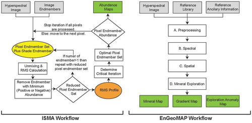
The EnMAP Geological MAPPER (EnGeoMAP)

EnGeoMAP in its application EnGeoMAP Base is a modular processing framework for the detection and characterization of geological surface material from future Environmental Mapping and Analysis Program (EnMAP) hyperspectral satellite data. It builds on the conceptual framework of expert systems, where a well-known spectral library, supplied by spectroscopy experts, is automatically compared (Mielke et al., 2016) to the unknown image spectra (Clark et al., 2003; Kokaly, 2012).

Its system is divided into a pre-processing module, a spectral module, a spatial module and can be supplied with additional mineral deposit-specific information in the mineral exploration module (Mielke et al., 2016) (Figure 6). The pre-processing module uses the geometric hull absorption feature characterization technique (Mielke et al., 2015) to retrieve the characteristic absorption bands in an image spectrum as well as in the reference library spectra that are supplied by the user. This automated band selection process, produces similar results to that being generated by an expert laboratory spectroscopist (Mielke et al., 2016). Previous studies have shown this by directly comparing the characteristic absorption features extracted manually by expert knowledge versus fully automated geometric hull technique (Mielke et al., 2016). In this study, the reference library is supplied by the aforementioned SSEE algorithm, which provides the necessary consistent data base to both algorithms EnGeoMAP and ISMA. The spectral module performs a best-weighted fit analysis of the pixel spectrum to the reference library, taking into account the position depth and overall shape of the characteristic absorption features only. Fitting with the full data spectrum is avoided to reduce erroneous results. The weighted fit values are retrieved for each library entry per image pixel spectrum. Next, a bound value least squares unmixing (BVLS) is performed with only those library endmembers that pass a user given threshold of 50% (Mielke et al., 2016). This process excludes endmembers from entering the unmixing process of each individual pixel, which falls under the 50% absorption feature correlation threshold. The spatial module creates the material maps from a user-supplied color table. Here the best fit and BVLS results are color-coded based on the highest best-weighted fit value (best-fit material map prior to the unmixing) and the highest abundant endmember (BVLS map after correlation thresholding and unmixing). In addition, spatial-spectral gradients are calculated from the unmixing results. Additional metadata maps are also computed that illustrate the position of the strongest absorption feature in the VNIR (up to 1 μm) and in the SWIR range (1–2.5 μm), as well as its value at the absorption maximum.

Results and discussion

Spatial–Spectral Endmember ExtractionThe derived endmembers represent mixtures of minerals in which iron content and lichen cover have a strong effect (Figure 7). Lichen and stunted vegetation grow selectively on specific lithologies, including gabbros, peridotite and basement gneiss. The most distinct spectral signatures were derived from vegetation, which in this area only, are a good proxy for gabbro and lherzolite rocks. It is apparent that the spectral mixture of rocks and vegetation are similar to the vegetation spectra where a slight peak at 0.56 µm and weak absorption at 0.64 µm are indicative of vegetation (Figure 7(c)). The spectral curves of lichen-covered mafic and ultramafic rocks show lichen-masking effects on spectral features in the 0.4–2 μm region; however, some absorption features from the underlying mineralogy are discernible in the 2.1–2.4 μm region (Figure 7(c)).

Figure 7. Spectral end-members used for ISMA and EnGeoMAP mapping methods. Outcrop related endmembers using (a) full range of spectral bands and (b) knowledge-based band selection. Vegetation and lichen related endmembers using (c) full range of spectral bands and (d) knowledge-based band selection. See Table 2 for detailed description of the selected spectral bands

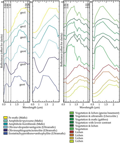
To better assess and interpret the image endmembers, reference spectra of hornblende, anthophyllite, actinolite, phlogopite, antigorite, olivine, enstatite, hypersthene and diopside minerals were selected from the USGS spectral library (http://speclab.cr.usgs.gov/) and convolved to response function of HyMAP data (Figure 8). It should, however, be noted that spectral mixing with vegetation and lichen endmembers as well as confusion between minerals with subtle differences are undoubted considering the course spatial resolution of HyMAP data, i.e. 20 m.

Figure 8. Comparison of HyMAP endmembers (solid lines) derived from SSEE with best matches from laboratory sample average spectra and mineral spectra taken from the USGS spectral library for (a,b) gabbro, (c,d) pyroxenite, (e,f) peridotite and (g,h) dunite samples. See Table 1 for detailed description of mineralogical composition of each sample determined from X-ray fluorescence analysis

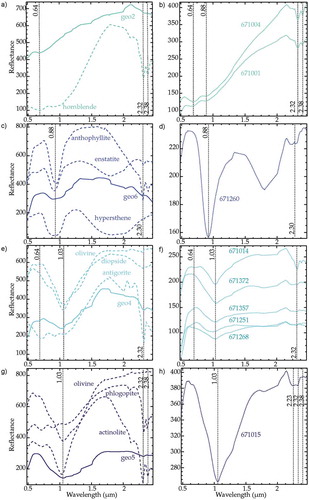
Mafic rocks have a higher reflectance than ultramafic rocks, with a maxima around 1.76–2.13 μm and distinct Fe features in VNIR around 0.64 and 0.88 μm (Figure 7(a)). Maxima around 1.76 μm is indicative of actinolite while maxima around 2.13 μm is indicative of hornblende. The shape of spectral as well as the wavelength position of Fe feature helps in differentiating these minerals. Actinolite Fe feature is around 1.03 μm while this feature is around 0.64 and 0.88 μm for hornblende. The Fe feature around 0.88 μm is usually masked by lichen coverage (Figure 7(c)). The SWIR spectral characteristics of these rocks are dictated by amphibole minerals as exemplified by hornblende in Figure 8. These SWIR absorption features are at 2.32 and 2.38 μm and both features are of the same order of magnitude (Figure 8(a,b)).

Ferrous (Fe⁺²) and ferric (Fe⁺³) iron in ultramafic rocks show distinct absorption features around 1.03 and 0.64 μm owing to minimal lichen cover on those substrates. Furthermore, a third absorption feature close to 0.88 μm is related to Fe⁺²/Fe⁺³ intervalence charge transfer (Figure 7). The ferrous iron content in the ultramafic rocks is dominant and complies with the deeper absorption band around 1.03 µm. For dunite, containing almost all olivine, only iron absorption feature at 1.03 µm is exhibited (Figure 8(g)). Pyroxene-rich peridotites show ferrous and minor ferric features (Figure 8(e,f)), while pyroxenites show an Fe⁺²/Fe⁺³ feature (Figure 8(c,d)). In SWIR, pyroxenites exhibit an Mg-OH feature around 2.30 µm related to anthophyllite (Figure 8(c)). The strong Mg-OH feature at 2.32 µm in peridotites is associated with serpentine (Figure 8(e)). Here, the image endmember that has been used for mapping dunite units shows two features around 2.30 and 2.38 µm, which are probably due to the presence of phlogopite/actinolite (Figure 8(g)). According to (Østergaard, 2011) quartz-rich gneiss xenoliths and diopside-mica-anthophyllite-actinolite alteration occur within pegmatitic pyroxenite unit in the northeastern part of the complex.

ISMA and EnGeoMAP Classification ResultsUsing the full range of spectral bands limits the overall spectral contrast between rock types. This presents a problem for spectral mixture analysis, where collinearity amongst endmembers can cause errors in abundance fractions. Improving spectral contrast, and in turn, minimizing potential collinearity problems requires band selection (Rogge et al., 2014b) that is weighted in favor of key spectral features (Figure 7(b,d)). This is achieved by applying a knowledge – driven band selection routine for ISMA and a purely data – driven band selection technique for EnGeoMAP method.

For ISMA method 16 VNIR and 16 SWIR bands (Table 2) are selected based on expert knowledge and field and laboratory spectral measurements (Figure 7(b,d)) to discriminate key rock units and map broad material classes (e.g. vegetation and lichens). The primary merit of selected VNIR bands is to differentiate between mafic and ultramafic units using the broad features around 0.88 and 1.03 μm in case of ultramafic units and 0.64 μm in case of mafic bodies. Other selected VNIR bands allow capturing the shape of overall spectral to map non-geological materials including rock incrusting lichens and vegetation that supress bedrock mineralogy. To capture the broad absorption features related to lichens the 1.73, 2.11, 2.30 µm are included in the selected bands (Rogge et al., 2014a; Salehi et al., 2017b).

Table 2. Spectral bands used for SSEE and ISMA, wavelength in µm

VNIR	0.562, 0.571, 0.586, 0.617, 0.633, 0.648, 0.663, 0.678, 0.740, 0.785, 0.888, 0.936, 1.030, 1.076, 1.091, 1.279
SWIR	1.658, 1.670, 1.732, 2.098, 2.116, 2.204, 2.220, 2.257, 2.274, 2.308, 2.324, 2.340, 2.357, 2.373, 2.389, 2.405

Using the selected bands for the image and the extracted endmembers from SSEE method, the unmixing process is then applied on the continuum removed HyMAP image mosaic that was aggregated to 20 m spatial resolution to simulate the ground sampling distance (GSD) of a spaceborne sensor, such as Sentinel-2. Figure 9 shows a comparison of classification results obtained from ISMA and EnGeoMAP approaches. Here ISMA classification map is generated by assigning each pixel to the geological endmember with the maximum fractional abundance (Figure 9(c)). The best fit and BVLS results are color-coded based on the highest best-weighted fit value and the highest abundant endmember, respectively (Figure 9(d,e)).

Figure 9. (a) HyMAP continuum removed RGB color composite highlighting the main mafic-ultramafic units. Red – ferric iron (0.64 μm); Green – Mg-OH (2.32 μm); and Blue – ferrous iron (1.03 μm). (b) False-colour composite image highlighting the abundance of vegetation in the area. Classification results for HyMAP data generated from (c) ISMA, (d) best fit and (e) BVLS methods

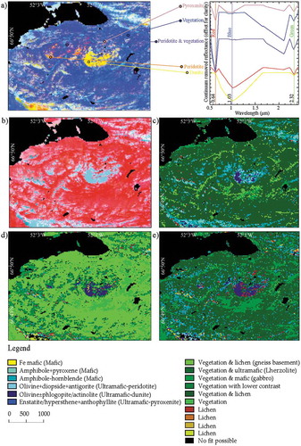
RGB color composite of continuum removed HyMAP image generated from ferric iron (0.64 µm), ferrous iron (1.03 µm) and Mg-OH (2.32 µm) bands highlights the exposed mafic and ultramafic units (Figure 9(a)). Within the ultramafic complex in the eastern dunite body, ferrous iron shows a high abundance, depicted as yellow color, whereby the ferric iron is lower abundant as compared to the western dunite. The reason could be that the eastern dunite block is less weathered than the residual part of the ultramafic complex since the Fe ³⁺ is the product of Fe ²⁺ oxidation resulting in rock weathering at the surface. Olivine-poorer peridotite zone (lherzolite and harzburgite) is shown by orange color due to deep antigorite feature around 2.32 µm, higher reflectance values around 0.64 µm and low reflectance values for ferrous iron (1.03 µm). The areas manifested in dark blue and purple colors (Figure 9(a)) are associated with oversaturation of the absorption bands with vegetation and partially lichen coverage (see red pixels in Figure 9(b)).

Figure 10 shows a comparison between the abundance maps generated for the main mafic and ultramafic endmembers (see geo2 to geo6 in Figure 7) using ISMA and EnGeoMAP methods. It is evident from Figure 10 that the map patterns of the ultramafic and mafic units for the entire study area are slightly different using each of these approaches. Comparison of RGB composites of abundance maps obtained from ISMA and EnGeoMAP for endmembers mafic-gabbro (geo2), peridotite (geo6) and dunite (geo5) shows a clear distinction of these units (Figure 10(f,l)).

Figure 10. Spectral unmixing results from ISMA and EnGeoMAP showing abundances for (a,g) geo2 – mafic (amphibole + pyroxene); (b,h) geo3 – mafic (amphibole – hornblende); (c,i) geo4 – peridotite (olivine + diopside + antigorite); (d,j) geo5 – dunite (olivine ± phlogopite/actinolite); and (e,k) geo6 – pyroxenite (enstatite/hypersthene + anthophyllite) endmembers. RGB color composites of abundances for (f) ISMA and (l) EnGeoMAP highlighting the main mafic-ultramafic units. Red – mafic (geo2); Green – peridotite; and Blue – dunite

The mapping results achieved for mafic – gabbro (geo2) unit are consistent with the existing geological map (Figure 10(a,g)). On the other hand, mafic (geo3) endmember shows correlation with both gabbro and peridotite units. There is also a lot of overlap with the quaternary unit using this endmember due to the lichen cover, which affects spectral recognition of its associated lithologies by imparting a subtle chlorophyll absorption feature near 0.6–0.7 μm. The results indicate that ISMA approach is less sensitive to this effect as compared to EnGeoMAP (Figure 10(b,h)).

As mentioned earlier, the study area host three ultramafic units, i.e. peridotite, pyroxenite and dunite rocks. EnGeoMAP maps both east and west dunites, while ISMA picks up only the eastern dunite (Figure 10(d,j)) and classifies the western dunite as peridotite (Figure 10(c)). Based on our observations from HyMap data the southern part of the western dunite shows characteristic features related to peridotite, while the rest of the outcrop is highly mixed with vegetation pixels (Figure 9(b)). Peridotite abundance map derived from EnGeoMAP corresponds better with the geological map, however there are slight differences between the geological map and the peridotite abundance maps regardless of the applied unmixing approach.

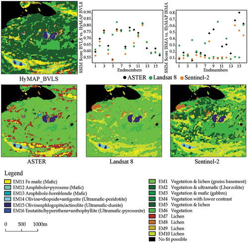
The HyMAP data are then convolved with the spectral response functions of Sentinel-2, ASTER and Landsat-8 OLI to evaluate the capabilities of these large swath width sensors in mapping ultramafic rocks in the Arctic region and in presence of abundant lichens. The extracted endmembers from SSEE method are resampled to the spectral response function of the simulated ASTER, Landsat-8 OLI, and Sentinel-2 data. The generated unmixing results are then compared to that from the 20 m HyMAP reference base (Figure 11). Direct comparison between the real multispectral dataset and the airborne HyMAP data was not carried out here. This is mainly because the time gap of at least 10 to 13 years between the airborne data (acquired in 2002) and actually available Landsat-8 and Sentinel-2 data is too large. To overcome this problem, we have tested the mapping approaches on the simulated datasets. Figure 11 shows the classification result for the different simulated multispectral data using BVLS unmixing approach, where the highest pixel abundance value determines the color of the pixels class, as in case of the USGS Tetracorder (Clark et al., 2003), MICA (Kokaly, 2012) and EnGeoMAP (Mielke et al., 2016). The visual resemblance between all sensors for the ultramafic class is striking. All sensors show a good overall performance in locating the major ultramafic bodies.

Figure 11. Classification results generated from BVLS for simulated ASTER, Landsat-8 OLI, and Sentinel-2. HyMAP BVLS and ISMA data are used as a reference base and similarity scores for each endmember and sensor to the HyMAP reference are indicated in the plot

Structural Similarity Index Measure (SSIM) for characterizing ISMA and EnGeoMAP

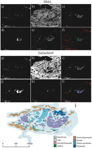
For HyMAP data, the binarized dunite, pyroxenite and peridotite images generated from the geological map are used as ground truths. The binarized outputs of ISMA, the EnGeoMAP weighted fitting (BFIT) and BVLS for these endmembers are quantitatively compared to the related ground truth, using the SSIM method (Wang et al., 2004). This method represents a sensitive measure to compare subtle differences between two images and provide a robust and quantitative similarity measure that considers the structure of the image as well (Wang et al., 2004). To assess the results for the whole ultramafic complex; the dunite, pyroxenite and peridotite abundance maps are merged and compared to the equivalent ground truth derived from the geological map (Table 3). The results imply that BVLS performs better than BFIT and ISMA for all classes. The similarity of ISMA to the dunite ground truth is 62.22%, whilst the similarity to EnGeoMAPs BVLS and best-weighted fit results are 75.37% (see Figure 12 & Table 3 for the results).

Table 3. Quantitative comparison between the results generated using different processing approaches with the reference image

Figure 12. a) The binarized dunite class from the geological map is used as ground truth. The binarized classification results for HyMAP data generated using b) ISMA, c) best fit, and d) BVLS methods for the dunite endmember

On the other hand, the BVLS results for pyroxenite endmember yield 83% similarity with the ground truth, while the related abundance map in Figure 10 implies differently. The reason is that if the image structure is mostly void (as in our case), SSIM overestimates the zero-valued non-class pixels. To overcome this problem, a direct correlation-based comparator is used for characterizing the results achieved from ISMA and EnGeoMAP (Table 3). Furthermore, to exclude the no-class pixels and only counting the similarity of the outputs with binary one from the ground truth image; we propose a hard measure, namely positive binary. Here a sum ratio between the product of result and reference and the reference sum is calculated as a measure for similarity between the two images (Table 3). The results suggest that EnGeoMAP performs better for mapping the dunite unit, while ISMA yields higher similarity for the other three classes.

The same approach is used for comparing the performance of spaceborne ASTER, Sentinel-2 and Landsat-8 OLI results with HyMAP reference data. Similarity scores for each endmember and sensor to the HyMAP reference are given in Figure 11. Considering the different sensors potential to map certain surface cover types, there are noticeable differences in the sensors overall similarity to the HyMAP reference data (Figure 11). ASTER performs well for all endmember entries with noticeable changes in the SWIR, whilst Sentinel-2 and Landsat-8 are mostly limited to a good performance in the VNIR. The numbers for the overall sensors performance for mapping the last two spectral endmembers, representing the ultramafic material are comparable to those from Platinum tailings in South Africa in (Mielke et al., 2014). Furthermore, EnGeoMAP shows higher similarity to the HyMAP BVLS reference image for the mafic units (endmembers 11 to 13, i.e. geo1, geo2 & geo3 in Figure 7), whilst ISMA performs better for mapping the ultramafic units (endmembers 14 to 16, i.e. geo4, geo5 & geo6 in Figure 7).

Conclusions

This study examines the possibility to extract valuable mineralogical and lithological information from airborne hyperspectral and spaceborne multispectral data where abundant rock encrusting lichens mask bedrock mineralogy. An airborne hyperspectral data covering 3.5 × 2.5 km² region coinciding with the Niaqornarssuit complex in West Greenland are aggregated to 20 m resolution that resembles the GSD of spaceborne sensors to provide a testbed with a reasonably large spectral mixing for the performance tests of ISMA and EnGeoMAP algorithms. In addition, band selection is used for optimizing the spectral unmixing using a knowledge – driven band selection routine, as in case of ISMA; and a purely data – driven band selection technique as in case of EnGeoMAP. For assessment of the results, we made extensive use of laboratory and field spectral measurements as well as XRF analysis to obtain geochemical data.

The map products generated from the aggregated scene capture the broad geological patterns and much of the lithologies shown in the geological map though some spatial and lithological discrimination is lost, as expected. Mafic (gabbro) and ultramafic units (dunite, peridotite, pyroxenite) are distinguished based on generally intense Mg-OH feature in short-wave-infrared (SWIR) and ferric and ferrous-iron absorption features in the visible and near-infrared (VNIR). Ferrous (Fe⁺²) and ferric (Fe⁺³) features around 1.03 and 0.64 μm are key indicators of the ultramafic units owing to minimal lichen cover on those substrates. Furthermore, a third absorption feature close to 0.88 μm is related to Fe⁺²/Fe⁺³ intervalence charge transfer. For dunite, containing almost all olivine, only Fe⁺² feature at 1.03 µm is exhibited. This unit often shows SWIR features around 2.32 and 2.38 μm related to phlogopite and-or actinolite minerals. Pyroxene-rich peridotites show Fe⁺² and minor Fe⁺³ features, while pyroxenites show an Fe⁺²/Fe⁺³ feature around 0.88 μm. Antigorite and anthophyllite minerals are critical for discrimination of peridotite and pyroxenite units with slightly different Mg-OH features around 2.32 and 2.30 µm, respectively. Mafic rocks have a higher reflectance than ultramafic rocks, with a pick around 2.13 μm and distinct Fe features in VNIR around 0.64 and 0.88 μm. The Fe feature around 0.88 μm is usually masked by lichen coverage. The SWIR spectral characteristics of these rocks are dictated by amphibole minerals with absorption features at 2.32 and 2.38 μm. These results indicate the importance of analyzing the spectral shape and albedo, as well as analyzing specific VNIR and SWIR spectral features for mapping mafic-ultramafic units in weathered terrain.

Next, the performance of aforementioned unmixing approaches is tested for simulated ASTER, Landsat-8 and Sentinel-2 spaceborne dataset. The results suggest that unmixing methods applied to ASTER data are more effective in differentiating mafic and ultramafic rocks as compared to the Landsat-8 and Sentinel-2 data. The dunite and peridotite ultramafic rocks are delineated using ASTER data. In addition, one of the lichen endmembers (EM7) shows a good correlation with olivine-peridotite unit in the southern part of west dunite. The presence of abundant vegetation and lichen is more problematic in landsat-8 and sentinel-2 data and only dunite ultramafic unit is mapped using these sensors. For these two sensors, lichen endmember (EM8) partially corresponds with the peridotite unit.

The achieved results demonstrate that aggregated data will be able to provide a large-scale reconnaissance (e.g. less detailed) mapping capability and useful exploration information of geologic materials (discrimination of mafic and ultramafic rock units in weathered terrain), showing the usefulness of next generation hyperspectral spaceborne sensors such as HISUI, EnMAP and PRISMA. Furthermore, we were able to assess the value of satellite sensor systems to support geological mapping and mineral exploration of ultramafic complexes in the arctic regions that become ever more important as more sophisticated spaceborne sensors become available, with NASA and ESA leading the way to new earth observation missions such as HySPIRI, Landsat-9 and new additions to ESA’s Copernicus Sentinel fleet.

Acknowledgment

The authors would like to thank the three anonymous reviewers whose comments have greatly improved this manuscript. The Geocenter Denmark is thanked for funding the Geological Remote Sensing PhD project of which this work is a part. Further, Geological Survey of Denmark and Greenland is gratefully acknowledged for providing the airborne hyperspectral dataset. We sincerely thank the 21st North Company for access to the rock samples and expedition reports. Agnieszka Kuras and the entire group in the German Research Centre for Geosciences are thanked for their support with the XRF measurements and sample preparation.

Disclosure statement

No potential conflict of interest was reported by the authors.

Additional information

Funding

This work was supported by the Geocenter Danmark [2-2014].

References

- Bedini, E. (2009). Mapping lithology of the Sarfartoq carbonatite complex, southern West Greenland, using HyMap imaging spectrometer data. Remote Sensing of Environment , 113 (6), 1208–1219. https://doi.org/10.1016/j.rse.2009.02.007
- Bedini, E. (2011). Mineral mapping in the Kap Simpson complex, central East Greenland, using HyMap and ASTER remote sensing data. Advances in Space Research , 47(1), 60–73. https://doi.org/10.1016/j.asr.2010.08.021
- Bedini, E. (2012). Mapping alteration minerals at Malmbjerg molybdenum deposit, central East Greenland, by Kohonen self-organizing maps and matched filter analysis of HyMap data. International Journal of Remote Sensing , 33(4), 939–961. https://doi.org/10.1080/01431161.2010.542202
- Buckley, S. J. , Kurz, T. H. , Howell, J. A. , & Schneider, D. (2013). Terrestrial lidar and hyperspectral data fusion products for geological outcrop analysis. Computers & Geosciences , 54, 249–258. https://doi.org/10.1016/j.cageo.2013.01.018
- Budkewitsch, P. , Staenz, K. , Neville, R. , Rencz, A. , & Sangster, D. (2000). Spectral signatures of carbonate rocks surrounding the Nanisivik MVT Zn-Pb mine and implications of hyperspectral imaging for exploration in Arctic environments. In Ore Deposit Workshop: New Ideas for a New Millennium, Technical Volume .
- Clark, R. N. , Swayze, G. A. , Livo, K. E. , Kokaly, R. F. , Sutley, S. J. , Dalton, J. B. , McDougal, R. R. , & Gent, C. A. (2003). Imaging spectroscopy: Earth and planetary remote sensing with the USGS Tetracorder and expert systems. Journal of Geophysical Research: Planets , 108(E12), 5-1 - 5-44. https://doi.org/10.1029/2002JE001847
- Cocks, T. , Jenssen, R. , Stewart, A. , Wilson, I. , & Shields, T. (1998). The HyMapTM airborne hyperspectral sensor: The system, calibration and performance. Proceedings of the 1st EARSeL workshop on Imaging Spectroscopy (pp. 37–42), Presented at 1st EARSEL Workshop on Imaging Spectroscopy, Zurich, October 1998.
- Gao, L. , Yao, D. , Li, Q. , Zhuang, L. , Zhang, B. , & Bioucas-Dias, J. (2017). A new low-rank representation based hyperspectral image denoising method for mineral mapping. Remote Sensing , 9(11), 1145. https://doi.org/10.3390/rs9111145
- Garde, A. A. , & Marker, M. (2010). Geological map of Greenland, 1:500 000, Søndre Strømfjord – Nuussuaq, Sheet 1 (2nd ed.). In n. edition (Ed.). Geological Survey of Denmark and Greenland.
- Gothenborg, J. , & Keto, L. (1980). Report on the aerial reconnaissance between Sukkertoppen Ice Calot and Nordenskiölds Gletscher 1977 (p. 84). Unpublished report, Kryolitselskabet Øresund A/S, Copenhagen, Denmark (in archives of Geological Survey of Denmark and Greenland, GEUS Report File 20071)
- Harris, J. R. , Rogge, D. , Hitchcock, R. , Ijewliw, O. , & Wright, D. (2005). Mapping lithology in Canada’s Arctic: Application of hyperspectral data using the minimum noise fraction transformation and matched filtering. Canadian Journal of Earth Sciences , 42(12), 2173–2193. https://doi.org/10.1139/e05-064
- Heinz, D. C. (2001). Fully constrained least squares linear spectral mixture analysis method for material quantification in hyperspectral imagery. IEEE Transactions on Geoscience and Remote Sensing , 39 (3), 529–545. https://doi.org/10.1109/36.911111
- Huo, H. , Ni, Z. , Jiang, X. , Zhou, P. , & Liu, L. (2014). Mineral mapping and ore prospecting with hymap data over Eastern Tien Shan, Xinjiang uyghur autonomous region. Remote Sensing , 6(12), 11829. https://doi.org/10.3390/rs61211829
- Jensen, S. M. , Hansen, H. , Secher, K. , Steenfelt, A. , Schjøth, F. , & Rasmussen, T. M. (2002). Kimberlites and other ultramafic alkaline rocks in the Sisimiut–Kangerlussuaq region, southern West Greenland. Geology of Greenland Survey Bulletin , 191 (2002), 57–66. https://eng.geus.dk/media/12936/gsb191p57-66.pdf
- Kokaly, R. F. (2012). Spectroscopic remote sensing for material identification, vegetation characterization, and mapping. Algorithms and Technologies for Multispectral, Hyperspectral, and Ultraspectral Imagery XVIII (p. 839014). International Society for Optics and Photonics.
- Kopačková, V. , & Koucká, L. (2017). Integration of absorption feature information from visible to longwave infrared spectral ranges for mineral mapping. Remote Sensing , 9(10), 1006. https://doi.org/10.3390/rs9101006
- Kruse, F. , & Perry, S. (2013). Mineral mapping using simulated worldview-3 short-wave-infrared imagery. Remote Sensing , 5(6), 2688–2703. https://doi.org/10.3390/rs5062688
- Larsen, L. M. , & Rex, D. C. (1992). A review of the 2500 ma span of alkaline-ultramafic, potassic and carbonatitic magmatism in West Greenland. Lithos , 28(3–6), 367–402. https://doi.org/10.1016/0024-4937(92)90015-Q
- Lorenz, S. , Salehi, S. , Kirsch, M. , Zimmermann, R. , Unger, G. , Vest Sørensen, E. , & Gloaguen, R. (2018). Radiometric correction and 3d integration of long-range ground-based hyperspectral imagery for mineral exploration of vertical outcrops. Remote Sensing , 10(2), 176. https://doi.org/10.3390/rs10020176
- Marion, R. , & Carrère, V. (2018). Mineral mapping using the automatized gaussian model (AGM)—Application to two industrial french sites at Gardanne and Thann. Remote Sensing , 10(1), 146. https://doi.org/10.3390/rs10010146
- Mielke, C. , Boesche, N. , Rogass, C. , Kaufmann, H. , Gauert, C. , & de Wit, M. (2014). Spaceborne mine waste mineralogy monitoring in South Africa, applications for modern push-broom missions: Hyperion/OLI and EnMAP/Sentinel-2. Remote Sensing , 6(8), 6790–6816. https://doi.org/10.3390/rs6086790
- Mielke, C. , Boesche, N. K. , Rogass, C. , Kaufmann, H. , & Gauert, C. (2015). New geometric hull continuum removal algorithm for automatic absorption band detection from spectroscopic data. Remote Sensing Letters , 6(2), 97–105. https://doi.org/10.1080/2150704X.2015.1007246
- Mielke, C. , Rogass, C. , Boesche, N. , Segl, K. , & Altenberger, U. (2016). EnGeoMAP 2.0—Automated hyperspectral mineral identification for the German EnMAP space mission. Remote Sensing , 8(2), 127. https://doi.org/10.3390/rs8020127
- Notesco, G. , Ogen, Y. , & Ben-Dor, E. (2016). Integration of hyperspectral shortwave and longwave infrared remote-sensing data for mineral mapping of Makhtesh Ramon in Israel. Remote Sensing , 8(4), 318. https://doi.org/10.3390/rs8040318
- Østergaard, C. (2011). 21st NORTH - 2010 field work, qaqortorsuaq (Ikertoq) .
- Rogass, C. , Segl, K. , Mielke, C. , Fuchs, Y. , & Kaufmann, H. (2014). EnGeoMap—A geological mapping tool applied to the EnMAP mission. Ukrainian Journal of Remote Sensing, 1 (2014), (pp. 12–17)
- Rogge, D. , Rivard, B. , Laakso, K. , & Segl, K. (2014a). Mapping Ni-Cu (PGE) bearing ultramafic rocks and associated gossans with airborne and simulated EnMAP satellite hyperspectral imagery. 2014 IEEE geoscience and remote sensing symposium (pp. 278–281). Nunavik, Canada: IEEE
- Rogge, D. , Rivard, B. , Segl, K. , Grant, B. , & Feng, J. (2014b). Mapping of NiCu–PGE ore hosting ultramafic rocks using airborne and simulated EnMAP hyperspectral imagery, Nunavik, Canada. Remote Sensing of Environment , 152, 302–317. https://doi.org/10.1016/j.rse.2014.06.024
- Rogge, D. M. , Bachmann, M. , Rivard, B. , & Feng, J. (2012). Spatial sub-sampling using local endmembers for adapting OSP and SSEE for large-scale hyperspectral surveys. IEEE Journal of Selected Topics in Applied Earth Observations and Remote Sensing , 5(1), 183–195. https://doi.org/10.1109/JSTARS.2011.2168513
- Rogge, D. M. , Rivard, B. , Zhang, J. , & Feng, J. (2006). Iterative spectral unmixing for optimizing per-pixel endmember sets. IEEE Transactions on Geoscience and Remote Sensing , 44(12), 3725–3736. https://doi.org/10.1109/TGRS.2006.881123
- Rogge, D. M. , Rivard, B. , Zhang, J. , Sanchez, A. , Harris, J. , & Feng, J. (2007). Integration of spatial–spectral information for the improved extraction of endmembers. Remote Sensing of Environment , 110(3), 287–303. https://doi.org/10.1016/j.rse.2007.02.019
- Rosa, D. , Dewolfe, M. , Guarnieri, P. , Kolb, J. , LaFlamme, C. , Partin, C. , Salehi, S. , Vest Sørensen, E. , Thaarup, S. , Thrane, K. , & Zimmermann, R. (2017). Architecture and mineral potential of the paleoproterozoic Karrat Group, West Greenland. Results of the 2016 season . Geological Survey of Denmark and Greenland.
- Salehi, S. (2018). Potentials and challenges for hyperspectral mineral mapping in the Arctic: Developing innovative strategies for data acquisition and integration. Department of geosciences and natural resource management. Copenhagen university.
- Salehi, S. , Lorenz, S. , Vest Sørensen, E. , Zimmermann, R. , Fensholt, R. , Henning Heincke, B. , Kirsch, M. , & Gloaguen, R. (2018). Integration of vessel-based hyperspectral scanning and 3D-photogrammetry for mobile mapping of steep coastal cliffs in the arctic. Remote Sensing , 10(2), 175. https://doi.org/10.3390/rs10020175
- Salehi, S. , Mielke, C. , Pedersen, C. B. , & Olsen, S. D. (2019a). Comparison of ASTER and Sentinel-2 datasets for geological mapping: A case study from North-East Greenland. Geological Survey of Denmark and Greenland Bulletin , 43. https://doi.org/10.34194/GEUSB-201943-02-05
- Salehi, S. , Rogge, D. , Rivard, B. , Heincke, B. H. , & Fensholt, R. (2017b). Modeling and assessment of wavelength displacements of characteristic absorption features of common rock forming minerals encrusted by lichens. Remote Sensing of Environment , 199, 78–92. https://doi.org/10.1016/j.rse.2017.06.044
- Salehi, S. , Sørensen, E. V. , Rosa, D. , Lode, S. , Guarnieri, P. , Kokfelt, T. F. , & Bernstein, S. (2019b). Helicopter-borne remote sensing for geological mapping in the Arctic terrain. 12th fennoscandian exploration and mining (FEM 2019) , Levi, Lapland, Finland
- Salehi, S. , & Thaarup, S. M. (2018). Mineral mapping by hyperspectral remote sensing in West Greenland using airborne, ship-based and terrestrial platforms. Geological Survey of Denmark and Greenland Bulletin , 41 (2018), 47–50. https://doi.org/10.34194/geusb.v41.4339
- Schläpfer, D. , & Richter, R. (2002). Geo-atmospheric processing of airborne imaging spectrometry data. Part 1: Parametric orthorectification. International Journal of Remote Sensing , 23(13), 2609–2630. https://doi.org/10.1080/01431160110115825
- Secher, K. , & Larsen, L. M. (1980). Geology and mineralogy of the Sarfartoq carbonatite complex, southern West Greenland. Lithos , 13(2), 199–212. https://doi.org/10.1016/0024-4937(80)90020-1
- Simard, R.-L. , Bliss, I. , & Vaillancourt, C. (2014). Geology report – Licences 2010/17, 2013/28 and 2013/27 . Northernshield resources inc.
- Tukiainen, T. , & Krebs, J. D. (2004). Mineral resources of the Precambrian shield of central West Greenland (66 to 70 15ʹN), Part 4. Mapping of kimberlitic rocks in West Greenland using airborne hyperspectral data . Geological Survey of Denmark and Greenland (GEUS) report 2004 (45).
- Tukiainen, T. , Krebs, J. D. , Kuosmanen, V. , Laitinen, J. , & Schäffer, U. (2003). Field and laboratory reflectance spectra of kimberlitic rocks, 0.35-2.5 M [my] m . GEUS.
- Tukiainen, T. , & Thomassen, B. (2010). Application of airborne hyperspectral data to mineral exploration in North-East Greenland. Geological Survey of Denmark and Greenland Bulletin , 20 (2010), 71–74. https://doi.org/10.34194/geusb.v20.4982
- Tukiainen, T. , & Thorning, L. (2005). Detection of kimberlitic rocks in West Greenland using airborne hyperspectral data: The HyperGreen 2002 project. Geological Survey of Denmark and Greenland Bulletin , 7 (2005), 69–72. https://doi.org/10.34194/geusb.v7.4845
- Wang, Z. , Bovik, A. C. , Sheikh, H. R. , & Simoncelli, E. P. (2004). Image quality assessment: From error visibility to structural similarity. IEEE Transactions on Image Processing , 13(4), 600–612. https://doi.org/10.1109/TIP.2003.819861