Dimensionality reduction method for hyperspectral image analysis based on rough set theory

ABSTRACT

High-dimensional features often cause computational complexity and dimensionality curse. Feature selection and feature extraction are the two mainstream methods for dimensionality reduction. Feature selection but not feature extraction can preserve the critical information and maintain the physical meaning simultaneously. Herein, we proposed a dimensionality reduction method based on rough set theory (DRM-RST) for feature selection. We defined the hyperspectral image as a decision system, extracted the features as decision attributes, and selected the effective features based on information entropy. We used the Washington D.C. Mall dataset and New York dataset to evaluate the performance of DRM-RST on dimensionality reduction. Compared with full band classification, 184 or 185 redundant bands were removed in DRM-RST, respectively. DRM-RST achieved similar accuracy (overall accuracy >94%) by SVM classifier and reduced computing time by about 85%. We further compared the dimensionality reduction efficiency of DRM-RST against other popular methods, including ReliefF, Sequential Backward Elimination (SBE) and Information Gain (IG). The Producer’s accuracy (PA) and User’s accuracy (UA) of DRM-RST was greater than that of ReliefF and IG. DRM-RST showed greater stability of accuracy than SBE in dimensionality reduction when using for different datasets. Collectively, this study provides a new method for dimensionality reduction that can reduce computational complexity and alleviate dimensionality curse.

KEYWORDS:

• Hyperspectral image
• dimensionality reduction
• feature selection
• rough set theory

Introduction

Hyperspectral imaging is an emerging technology that integrates conventional imaging and spectroscopy to obtain a wealth of spectral information. It can provide the hyperspectral images with a large number of spectral bands. Hyperspectral imaging has advanced the application of remote sensing in many fields, such as estuarine and coastal water quality estimation (Brando & Dekker, 2003), wetland vegetation investigation (Adam et al., 2010) and coral reef feature identification (Mohanty et al., 2016). Hyperspectral imaging can detect and classify the spatial information at high accuracy. However, the high-dimensional feature often causes computational complexity and dimensionality curse (Ferrari et al., 2013; Gu et al., 2017; Sakarya, 2014). In many cases, it is not required to process the information of all spectral bands since many bands are highly correlated. Thus, it is required to remove redundant bands and decrease computational complexity.

Dimensionality reduction is an important pre-processing step in hyperspectral image analysis. It decreases computational complexity and ameliorates statistical ill conditioning by discarding redundant features. Two mainstream methods are available for dimension reduction, including feature extraction and feature selection (Bioucas-Dias et al., 2013; Yin et al., 2012). Feature extraction transforms the original features of hyperspectral images to construct lower-dimension feature spaces, which can be achieved by independent component analysis (ICA) (Wang, 2006), fisher’s linear discriminant analysis (FLDA) (Wu et al., 2017), graph embedding analysis (J.P. Guo et al., 2020) and principle component analysis (PCA) (Jolliffe, 1986). Feature extraction preserves the critical information of hyperspectral image. However, it alters the physical meaning of each spectral band (Dash & Liu, 2000).

Feature selection not only preserves the critical information of hyperspectral image, but also maintains the physical meaning of each spectral band. Several methods have been used for feature selection, including ReliefF (Peker et al., 2015), sequential forward search (SFS) (Lee et al., 2017) and sequential backward elimination (SBE) (Vergara & Estévez, 2014). ReliefF method estimates the optimal attributes relying on how well their values distinguish among the instances that are near each other (Kira & Rendell, 1992). SFS method selects the best attribute at first, then the second best, and so forth, trying to add the possible attribute to the one previously selected, until no improvement is achieved when adding a new attribute. SBE method aims to select a subset of size k among n variables (k < n), which maximizes the performance of the predictor, removing one feature at a time until k features remain (Maldonado & Weber, 2009). ReliefF is highly dependent on data samples. Many small data samples are sampled from the data. By contrast, SFS and SBE choose the best band combination of hyperspectral images through the iterative process. The reduction performances of these methods, such as accuracy and computing time, display highly variable for different datasets (Huang & He, 2005).

As for feature selection, the selection of possible band combinations is a critical issue. Band combination selection is a vague and quantitative problem. Rough set theory is a mathematical tool for dealing with the vague, imprecise and uncertain data (Liu et al., 2010). It has been applied successfully in the fields characterized by vagueness and uncertainty (Cervante et al., 2013; Yellasiri et al., 2007; Z.H. Guo et al., 2016). However, the application of rough set theory in dimensionality reduction is still unavailable. In this study, we proposed a dimensionality reduction method for hyperspectral image processing based on rough set theory (DRM-RST). DRM-RST can reduce computational complexity and alleviate dimensionality curse during hyperspectral image processing.

Material and method

Material

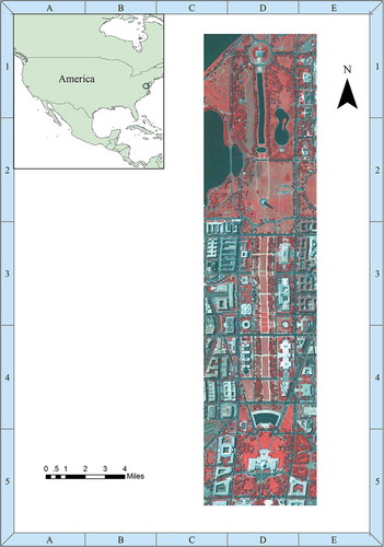
The first hyperspectral image dataset was acquired using the Hyperspectral Digital Imagery Collection Experiment (HYDICE) sensor and collected over Washington D.C. Mall on 23 August 1995. This scene consists of 1280 × 307 pixels and covers the 401.2881 ~ 2473.16 nm range with 191 spectral bands at approximately 10-nm spectral resolution and 3-m spatial resolution. Figure 1 shows the image of the data cube at the spectral band #60, #27 and #17.

Figure 1. Hyperspectral image of Washington D.C. Mall

(Spectral band #60, 27 and 17). The original image is available at http://lesun.weebly.com/hyperspectral-data-set.html.

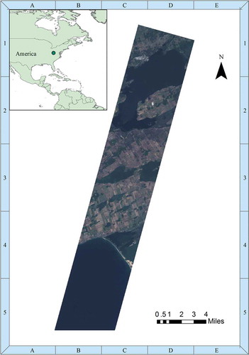
The second hyperspectral image dataset was acquired using the EO-1 Hyperion scene and collected over New York on 25 August 2001. This scene consists of 613 × 1335 pixels and covers the 400 ~ 2500 nm range with 198 spectral bands at approximately 10-nm spectral resolution and 30-m spatial resolution. Figure 2 shows the image of the data cube at the spectral band #29, #20 and #12.

Figure 2. Hyperspectral image of New York

(Spectral band #29, 20 and 12). The original image is available at https://earthexplorer.usgs.gov/.

Method

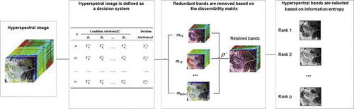
Figure 3 is the flow chart of DRM-RST method. The hyperspectral image is defined as a decision system, S*. The bands of hyperspectral image are recognized as the condition attributes, B. Then, the redundant bands are removed based on the discernibility matrix, which is deduced by the decision system, S*. Finally, the retained bands are ranked by calculating the information entropy of each band, and the required bands are selected according to the sequence of ranked bands.

Figure 3. Flow chart of DRM-RST method

Step 1: decision system definition

Hyperspectral image is defined as a decision system. Let $S=(U,A,V,F)$ be an information system, where $U=\{x_1,x_2,\cdots ,x_n\}$ is a finite set of objects (pixels in the image), which is called sample space. $A=\{a_1,a_2,\cdots ,a_m\}$ is a set of attributes; $\mathrm{\forall }a\in A$ determines a function $f=U\times A\to V$. $V=\bigcup _{a\in B}{V_{a_i}}_{\hspace{0.17em}}$, where $V_{a_i}$ is the set of values of$a_i$. A decision system is a particular case of information system. $B$ is a condition attribute, $D$is a decision attribute, where $A=B\cup D$ and$B\cap D=\mathrm{\varnothing }$.

The decision system is denoted as $S^{\ast }=(U,A=B\cup D,V,f)$. $A$ is a set of attributes, which the element of $B=\{B_1,B_2,\cdots ,B_m\}$ is a condition attribute and $D=\{d_i\}$ is a decision attribute. B and D represent the set of spectral bands and the type of a sample pixel, respectively. Table 1 is the structure of decision system.

Table 1. Decision system of hyperspectral image

	Condition attribute (B)
U	B1	B2	…	Bm	Decision attributes (D)
$x1$	$V_{B_1}^{x_1}$	$V_{B_2}^{x_1}$	…	$V_{B_m}^{x_1}$	$V_d^{x_1}$
$x2$	$V_{B_1}^{x_2}$	$V_{B_2}^{x_2}$	…	$V_{B_m}^{x_2}$	$V_d^{x_2}$
…	…	…	…	…	…
$xn$	$V_{B_1}^{x_n}$	$V_{B_2}^{x_n}$	…	$V_{B_m}^{x_n}$	$V_d^{x_n}$

Step 2: removing redundant bands

Redundant bands are removed based on the discernibility matrix. The discernibility matrix represents the sets of attributes that discerns the pairs of objects (Skowron & Rauszer, 1992). It calculates the attribute reduction in rough set theory. Attribute reduction is an essential operation of decision system (Shu & Qian, 2015). In the decision system$S\ast =(U,A,V,f)$, B and D are the sets of attributes including equivalence relations over U. B-positive region can be defined as the equation (1)(1) $POSB(D)=\bigcup _{x\in U/D}\underset{\_}{B}(x)$(1) . It refers to that all objects of U can be classified to classes of U/D using the information contained within attribute B.

(1) $POSB(D)=\bigcup _{x\in U/D}\underset{\_}{B}(x)$(1)

If$PO{S}_B(D)=PO{S}_{(B-\{a\})}(D)$, the attribute a ($a_i\in B$) is relatively dispensable, where $B$ is a condition attribute. Otherwise, a is relatively indispensable in B.

Given$B\ast$ as a subset of B ($B\ast \subseteq B$), if every attributes a ($a\in B\ast$) is indispensable in B. $B\ast$is relatively independent in$S\ast$. If $B\ast$is relatively independent, and $PO{S}_{B^{\ast }}(D)=PO{S}_B(D)$, the subset B ($B\ast \subseteq B$) is called relative reduction in$S\ast$. The collection of all relatively indispensable attributes in B is called the relative core of B, denoted as$COR{E}_D(B)$. $COR{E}_D(B)$ is the union of matrix element defined as

(2) $COR{E}_D(B)=\{m_{ij}\in B,1\le i,j\le n\}$(2)

The discernibility matrix is focused on the ability of attribute subsets to distinguish the objects belonging to different classes. Here, we use the discernibility matrix to remove the redundant information. Discernibility matrix has the dimension$n\times n$, where n denotes the number of objects. An element$mij$for an object pair ($xi,xj$) is defined as

(3) $mij=\left\{\begin{array}{c}\left\{\begin{array}{c}a|a\in B:Va(xi)\ne Va(xj),D(xi)\ne D(xj)\},\\ xi,xj\in U\end{array}\right.\\ \mathrm{\varnothing },others\end{array}\right.$(3)

Because of symmetric, only half elements of discernibility matrix is computed, and the retained elements of this discernibility matrix elements are$\mathrm{\varnothing }$. The meaning of the matrix element$m_{ij}$ is that objects$x_i$ and$x_j$ can be distinguished by any attributes in $m_{ij}$. The pair ($x_i,x_j$) can be discerned if$m_{ij}\ne \mathrm{\varnothing }$. Table 2 shows the part result of discernibility matrix.

Table 2. Part result of discernibility matrix of decision attribute

U	$x1$	$x2$	$x3$	$x4$	$x5$	$\cdots$
$x1$	$\mathrm{\varnothing }$
$x2$	$m_{12}$	$\mathrm{\varnothing }$
$x3$	$m_{13}$	$m_{23}$	$\mathrm{\varnothing }$
$x4$	$m_{14}$	$m_{24}$	$m_{34}$	$\mathrm{\varnothing }$
$x5$	$m_{15}$	$m_{25}$	$m_{35}$	$m_{45}$	$\mathrm{\varnothing }$
…	…	…	…	…	…	…

Discernibility function corresponding to discernibility matrix above is defined as follow:

(4) ${\rho }^{\ast }=\wedge \{\vee m_{ij}\}$(4)

Where “$\wedge$” (disjunction), “$\vee$” (conjunction) are the propositional connectives in mathematical logic. They are read as “or” and “and”. Assume$m=\{B_1,B_3,\cdots B_K\}$,and $m$ denotes $B_1\vee B_3\vee \cdots \vee B_k$, This function${\rho }^{\ast }$ is disjunctive normal form of conjunction$mij$, which presents the removed bands (Yao & Zhao, 2009).

Step 3: hyperspectral band selection

Hyperspectral bands are selected based on the information entropy. The weight of retained bands is calculated based on the information entropy (Zhang & Jiang, 2008). According to the decision attribute (D), the sample space (U) is divided into different type of classifications. Given events$D_1,D_2,\cdots ,D_m$occurring with the probabilities$P(D_1),P(D_2),\cdots ,P(D_m)$, the average uncertainty associates with each event is defined by the information entropy

(5) $H(D)=H(D1,D2,\cdots ,Dm)=-\sum _{i=1}^{m}P\left(\frac{Di}{|U|}\right)log2P\left(\frac{Di}{|U|}\right)$(5)

The condition attribute (B) has n dimension. a is the value domain of B. For each$aj$ ($j=1,2,\cdots n$), the information entropy is defined by

(6) $H(a)=\sum _{i=1}^m\frac{uij}{|U|}\sum _{j=1}^{n}H(u1j,\cdots ,umj)=\sum _{j=1}^n\frac{u1j+u2j+\cdots +umj}{|U|}H(u1j,\cdots ,umj)$(6)

$uj$is the subset of U which contains all objects with the same value of $aj$. $uij$is the number of the objects with the classification of $Di$ type.

Based on the information entropy of each band, the retained bands are ranked in a descending sequence. The required bands can be selected according to the sequence of retained bands. Finally, a new spectral image with the lower dimension is created.

Experimental results

In this section, DRM-RST method is used for selecting the effective band combinations in the hyperspectral image. The result of dimensionality reduction is used for the classification of hyperspectral image. Two experiments were conducted to evaluate the performance of DRM-RST method on dimensionality reduction based on rough set theory.

In the experiment 1, DRM-RST method was compared against full band classification to estimate whether DRM-RST method preserved the critical information of hyperspectral images. In the experiment 2, DRM-RST method was compared against other dimensionality methods, including ReliefF, sequential backward elimination (SBE), and information gain (IG), to evaluate the performance of dimensionality reduction.

Dimensionality reduction for Washington D.C. Mall dataset by DRM-RST method

By visual interpretation, the hyperspectral image of Washington D.C. Mall sense was classified into 7 different land-covers, including water, artificiality, road, grass, shadow, forest and trail, which was considered as the value of decision attribute (D) of S*. And then, 10 training sampled pixels for each land-cover was selected as the training sampled pixels. The total number of training sampled pixels was 70, which accounted for 2/1000 of total pixels. Table 3 shows the part result of decision system from hyperspectral image of Washington D.C. Mall dataset.

Table 3. Decision system of Washington D.C. Mall dataset

	Condition attribute (B)
U	B1	B2	…	B191	Decision attributes (D)
$x1$	3432	3181	…	0	$\mathrm{W}\mathrm{a}\mathrm{t}\mathrm{e}\mathrm{r}$
$x2$	3293	3303	…	1	$\mathrm{W}\mathrm{a}\mathrm{t}\mathrm{e}\mathrm{r}$
…	…	…	…	…	…
$x70$	4778	4505	…	24	$Trail$

Based on the equation (3)(3) $mij=\left\{\begin{array}{c}\left\{\begin{array}{c}a|a\in B:Va(xi)\ne Va(xj),D(xi)\ne D(xj)\},\\ xi,xj\in U\end{array}\right.\\ \mathrm{\varnothing },others\end{array}\right.$(3) , the discernibility matrix with the size of 70 × 70 was generated. The result of discernibility function ρ* with the equation (4)(4) ${\rho }^{\ast }=\wedge \{\vee m_{ij}\}$(4) was the removed bands. 107 redundant bands were removed, while 84 bands were retained as below.

$\rho \ast =(\vee m1,2)\wedge (\vee m1,3)\wedge \cdots \wedge (\vee m190,191)$

_{={B1,B5,B8,B14,B17,B18,B20,B22,B27,B31~B35,B38,B40~B46,B48,B49,B50,B52~B58,B60,B62~B64,B66~B86,B88~B90,B92~B97,B101,B108,B110,B111,B113,B114~B117,B119,B120~B125,B128,B130,B150}}

Based on the equation 5(5) $H(D)=H(D1,D2,\cdots ,Dm)=-\sum _{i=1}^{m}P\left(\frac{Di}{|U|}\right)log2P\left(\frac{Di}{|U|}\right)$(5) and 6(6) $H(a)=\sum _{i=1}^m\frac{uij}{|U|}\sum _{j=1}^{n}H(u1j,\cdots ,umj)=\sum _{j=1}^n\frac{u1j+u2j+\cdots +umj}{|U|}H(u1j,\cdots ,umj)$(6) , the information entropy for each retained band was calculated. The bands were ranked according to the value of information entropy. In this study, the Top 7 bands were selected (Table 4). The reason why we selected seven bands was that the selected bands could be sufficient to accommodate the specific problem.

Table 4. Top seven selected bands of Washington D.C. Mall dataset

Band	B1	B130	B108	B150	B85	B14	B46
Information entropy	0.21	0.20	0.18	0.16	0.15	0.14	0.14

Dimensionality reduction for New York scene dataset by DRM-RST method

The hyperspectral image of New York sense was classified into 6 different land-covers as the domain U and the land-covers, including water, artificiality, bare, beach and forest, form the decision attribute D. And then, 10 training sampled pixels for each land-cover was selected as the training sampled pixels. The total number of the training sampled pixels was 60, which accounted for 1/1000 of total pixels.

Based on the equation (3)(3) $mij=\left\{\begin{array}{c}\left\{\begin{array}{c}a|a\in B:Va(xi)\ne Va(xj),D(xi)\ne D(xj)\},\\ xi,xj\in U\end{array}\right.\\ \mathrm{\varnothing },others\end{array}\right.$(3) , the discernibility matrix with the size of 60 × 60 was generated. The result of discernibility function ρ* with the equation (4)(4) ${\rho }^{\ast }=\wedge \{\vee m_{ij}\}$(4) was the removed bands. 163 redundant bands were removed, while 35 bands were retained as below.

$\rho \ast =(\vee m8,9)\wedge (\vee m8,10)\wedge \cdots \wedge (\vee m223,224)$

_{={B17~B21,B23,B24,B26,B28,B29,B31,B32,B34~B39,B43,B45,B46,B49,B51,B57,B77~B79,B80,B82~B84,B88,B93,B115,B116}}

And then, the 13 top bands were selected as shown in Table 5.

Table 5. Top 13 selected bands of New York dataset

Band		B116	B57	B115	B17	B80
Information entropy		0.17	0.13	0.11	0.10	0.10
Band	B82	B32	B49	B51	B83	B26
Information entropy	0.10	0.10	0.09	0.09	0.09	0.08

Result of experiment 1: comparing against full band classification

The classification result of hyperspectral image by the Support Vector Machine classification (SVM) classifier was created through full band classification as the true value. We calculated the overall accuracy (OA) to estimate whether DRM-RST method preserved the critical information of hyperspectral images. Compared with full band classification, DRM-RST method had a comparable overall accuracy in dimensionality reduction of hyperspectral image. However, the computing time of DRM-RST method was significantly shorter than that of full band classification. When using DRM-RST method, the computing time for Washington D.C. Mall dataset or New York dataset was 16.46 s or 38.96 s, respectively. Compared with full band classification, DRM-RST method decreased the computational complexity, showing >85% reduction of computing time (Table 6).

Table 6. Comparison of computing time and overall accuracy between full band selection and DRM-RST method

Dataset	Selected band	Computing time (s)	Overall accuracy (%)
Washington D.C. Mall dataset	7-band	16.46	95.15
	full band	76.41
New York dataset	13-band	38.96	94.14
	full band	289.5

Moreover, we used the length (the perimeter length of a land cover, L), area (the total area of a land cover, A), and shape index ($SI=L/\sqrt{A}$) to further estimate whether DRM-RST method preserved the most critical information of hyperspectral images. Shape index was mathematically scale independent, based on the ratio of the perimeter to the square root of area (Jorge & Garcia, 1997). The result showed that the classification result of DRM-RST method was nearly similar as the result of full band classification (Figure 4, 5, Table 7, and 8).

Figure 4. Classification result of Washington D.C. Mall dataset by full band classification and DRM-RST method. (a) Full band classification; (b) DRM-RST method

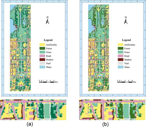
Figure 5. Classification results of New York dataset by full band classification and DRM-RST method. (a) Full band classification; (b) DRM-RST method

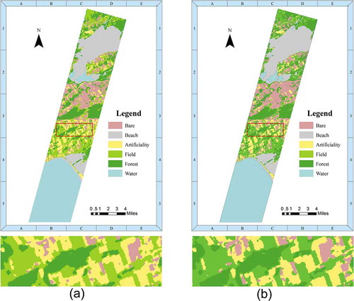
Table 7. Comparison of accuracy parameters of Washington D.C. Mall dataset by full band selection and DRM-RST method

	Length/km (10^5)		Area/km^2		Shape index (10^5)
Different land-cover	DRM-RST	Full band	DRM-RST	Full band	DRM-RST	Full band
Water	0.97	1.02	22.94	22.89	0.24	0.21
Artificiality	11.81	13.84	65.85	74.14	1.54	1.61
Road	16.94	15.56	70.62	61.89	2.05	1.98
Trail	2.84	2.73	6.94	7.24	1.06	1.01
Grass	17.10	17.27	106.52	106.68	1.66	1.67
Forest	13.92	14.36	67.01	65.07	1.68	1.78
Shadow	5.01	6.04	13.78	15.76	1.33	1.52
Total	68.59	70.82	353.66	353.67	9.56	0.21

Result of experiment 2: Comparing against other popular dimensionality reduction methods

We then compared the DRM-RST method against other popular dimensionality methods, including ReliefF, sequential backward elimination (SBE), information gain (IG) to estimate the performance of dimensionality reduction. We used two different parameters, Producer’s accuracy (PA) and User’s accuracy (UA), to estimate the performance of dimensionality reduction. Table 8 shows the selected bands by different dimensionality reduction methods for the Washington D.C. Mall dataset and New York scene dataset. Tables 9 and 10 shows the result of Producer’s accuracy (PA) and User’s accuracy (UA) for the two datasets respectively, which were classified by SVM classifier.

Table 8. Comparison of accuracy parameters of New York dataset by full band selection and DRM-RST method

	Length/km (10^5)		Area/km^2		Shape Index (10^5)
Different land-cover	DRM-RST	Full band	DRM-RST	Full band	DRM-RST	Full band
Water	1.32	1.39	88.36	88.7	0.14	0.15
Beach	1.9	2.08	59.19	59.43	0.25	0.27
Forest	5.75	5.84	44.7	48.35	0.86	0.84
Bare	7.01	5.82	56.03	38.13	0.94	0.94
Artificiality	3.05	6.3	10.27	28.09	0.95	1.19
Field	9.51	9.28	50.79	46.64	1.33	1.36
Total	28.54	30.71	309.34	309.34	4.47	4.75

Table 9. Selected bands by different dimensionality reduction methods

	Washington D.C. Mall dataset	New York dataset
Relief	89,97,95,94,93,96,90	31,29,80,87,79,83,82,85,86,88,30,81,32
SBE	191,72,1,53,102,134,35	224,173,170,177,172,176,122,168,124,127,79,125,166
IG	151,153,152,150,158,120,121	16,26,13,15,25,27,17,14,12,23,11,20,18
DRM-RST	1,130,108,150,85,14,46,8	116,57,115,17,80,93,84,82,32,49,51,83,26

Table 10. Comparison of PA and UA of Washington D.C. Mall dataset by different hyperspectral image reduction methods

		Different land-cover
	Parameter	Water	Artificiality	Road	Trail	Grass	Forest	Shadow	CI (95%)
Relief	PA	99.91	92.78	61.58	32.72	74.84	82.04	69.53	73.34 ± 15.2
	UA	92.08	59.57	81.47	62.29	92.82	82.19	92.79	80.46 ± 9.70
SBE	PA	99.23	96.48	93.62	86.77	94.76	98.12	91.81	94.40 ± 2.90
	UA	98.02	92.76	93.64	87.63	98.73	95.45	96.08	94.62 ± 2.57
IG	PA	99.51	93.85	59.04	26.7	90.26	91.63	83.84	77.83 ± 17.87
	UA	94.17	64.02	92.42	64.19	94.99	95.89	89.88	85.08 ± 9.92
DRM-RST	PA	99.57	97.42	94.21	72.83	96.03	94.04	90.73	92.12 ± 6.14
	UA	96.48	92.11	93.8	91.07	96.1	98.6	95.21	94.77 ± 1.80

From Tables 10 and 11, the PA and UA of DRM-RST method was greater than that of ReliefF and IG. DRM-RST method showed greater stability of reduction accuracy than SBE method. As for Washington D.C. Mall dataset, the PA and UA of DRM-RST method was approximate to the result of SBE method. As for New York dataset, the PA and UA of DRM-RST method was much greater than that of SBE method. These results suggest that DRM-RST is not dependent on the types of datasets and shows good stability of reduction accuracy.

Table 11. Comparison of PA and UA of New York dataset by different hyperspectral image reduction methods

		Different land-cover
	Accuracy parameter	Water	Beach	Forest	Bare	Artificiality	Field	CI (95%)
Relief	PA	99.34	97.16	79.36	86.64	38.04	92.66	82.2 ± 16.67
	UA	98.97	98.71	98.41	60.44	94.59	75.98	87.85 ± 10.87
SBE	PA	99.87	0.01	60.79	93.26	0.13	55.99	51.68 ± 31.81
	UA	60.04	100	80.32	43.33	47.06	60.26	65.17 ± 15.66
IG	PA	99.51	81.22	98.02	85.22	21.67	83.02	78.11 ± 20.98
	UA	99.75	99.28	70.58	60.53	83.14	87.41	83.45 ± 11.42
DRM-RST	PA	99.17	98.02	92.02	97.1	79.5	88.26	92.35 ± 5.50
	UA	99.38	98.65	93.91	80.46	91.75	93.27	92.90 ± 4.98

Conclusion

The high-dimensional data poses many problems, such as computational complexity, dimensionality curse, etc. (Ferrari et al., 2013; Gu et al., 2017). Due to the dimensionality curse and the diminishment of specificity in similarities between points in the hyperspectral image, the complexity of existing methods is exponential with respect to the number of dimensions (Sakarya, 2014). With increasing dimensionality, the existing methods become computationally intractable and inapplicable in the real application. Therefore, dimension reduction becomes a critical issue for hyperspectral image processing.

Feature selection is one of the mainstream methods for dimension reduction. It not only preserves the critical information but also maintains the physical meaning of hyperspectral image. The critical issue for feature selection is the selection of possible band combinations. However, band selection is a vague problem.

The major innovation of this study is that rough set theory is employed for dimension reduction of hyperspectral data. Rough set theory is an important method for vague, imprecise and uncertain data processing. In this study, we proposed a feature selection method for hyperspectral data analysis based on rough set theory (DRM-RST). Compared with full band classification, DRM-RST can remove the redundant bands and reduce computational burden. Compared with other popular dimensionality reduction methods, DRM-RST shows better reduction accuracy than IG and ReliefF and has greater stability of accuracy than SBE method in hyperspectral data analysis. Collectively, rough set theory-based feature selection has great potentials for dimensionality reduction of hyperspectral data.

Acknowledgments

This work was generously supported by the grants from the Capacity Development for Local College Project (Grant No. 19050502100 to W.Z.H.). The authors declare no conflicts of interest.

Disclosure statement

The authors declare no conflict of interest.

Additional information

Funding

This work was supported by the National Natural Science Foundation of China [41501419,41671431]; Capacity Development for Local College Project [17050501900, 19050502100].

References

- Adam, E. , Mutanga, O. , & Rugege, D. (2010). Multispectral and hyperspectral remote sensing for identification and mapping of wetland vegetation: A review. Wetlands Ecology & Management , 18(3), 281–296. https://doi.org/10.1007/s11273-009-9169-z
- Bioucas-Dias, J. M. , Plaza, A. , Camps-Valls, G. , Scheunders, P. , Nasrabadi, N. , & Chanussot, J. (2013). Hyperspectral remote sensing data analysis and future challenges. IEEE Geoscience and Remote Sensing Magazine , 1(2), 6–36. https://doi.org/10.1109/MGRS.2013.2244672
- Brando, V. E. , & Dekker, A. G. (2003). Satellite hyperspectral remote sensing for estimating estuarine and coastal water quality. IEEE Transactions on Geoscience and Remote Sensing , 41(6), 1378–1387. https://doi.org/10.1109/TGRS.2003.812907
- Cervante, L. , Xue, B. , Shang, L. , & Zhang, M. J. (2013). Binary particle swarm optimisation and rough set theory for dimension reduction in classification. In 2013 IEEE Congress on Evolutionary Computation , 2428–2435. https://doi.org/10.1109/CEC.2013.6557860
- Dash, M. , & Liu, H. (2000). Feature selection for clustering. Knowledge Discovery and Data Mining, Proceedings , 1805, 110–121. https://doi.org/10.1007/3-540-45571-X_13
- Ferrari, C. , Foca, G. , & Ulrici, A. (2013). Handling large datasets of hyperspectral images: Reducing data size without loss of useful information. Analytica Chimica Acta , 802(13), 29–39. https://doi.org/10.1016/j.aca.2013.10.009
- Gu, Y. F. , Chanussot, J. , Jia, X. P. , & Benediktsson, J. A. (2017). Multiple kernel learning for hyperspectral image classification: A review. IEEE Transactions on Geoscience and Remote Sensing , 55(11), 6547–6565. https://doi.org/10.1109/TGRS.2017.2729882
- Guo, J. P. , Yang, Y. Y. , Yi, Z. , Lv, J. C. , Mao, Q. R. , & Zhan, Y. Z. (2020). Discriminative globality and locality preserving graph embedding for dimensionality reduction. Expert Systems with Applications , 144(15), 113079. https://doi.org/10.1016/j.eswa.2019.113079
- Guo, Z. H. , Wang, H. , Du, X. M. , Chen, Y. F. , Yang, Y. , & Sheng, G. H. (2016). GIS partial discharge pattern recognition based on dimension reduction based on rough set theory. DEStech Transactions on Environment, Energy and Earth Sciences, (Peem) . https://doi.org/10.12783/dteees/peem2016/5028
- Huang, R. , & He, M. Y. (2005). Band selection based on feature weighting for classification of hyperspectral data. IEEE Geoscience and Remote Sensing Letters , 2(2), 156–159. https://doi.org/10.1109/LGRS.2005.844658
- Jolliffe, I. T. (1986). Principal component analysis and factor analysis. Principal Component Analysis , 115–128. https://doi.org/10.1007/978-1-4757-1904-8_7
- Jorge, L. A. B. , & Garcia, G. J. (1997). A study of habitat fragmentation in Southeastern Brazil using remote sensing and geographic information systems (GIS). Forest Ecology and Management , 98(1), 35–47. https://doi.org/10.1016/S0378-1127(97)00072-8
- Kira, K. , & Rendell, L. A. (1992). A practical approach to feature selection. Machine Learning Proceedings 1992 , 249–256. https://doi.org/10.1016/B978-1-55860-247-2.50037-1
- Lee, J. L. , Park, D. , & Lee, C. H. (2017). Feature selection algorithm for intrusions detection system using sequential forward search and random forest classifier. Ksii Transactions on Internet and Information Systems , 11(10), 5132–5148.
- Liu, L. , Zhou, J. Z. , An, X. L. , Zhang, Y. C. , & Yang, L. (2010). Using fuzzy theory and information entropy for water quality assessment in Three Gorges region, China. Expert Systems with Applications , 37(3), 2517–2521. https://doi.org/10.1016/j.eswa.2009.08.004
- Maldonado, S. , & Weber, R. (2009). A wrapper method for feature selection using support vector machines. Information Sciences , 179(13), 2208–2217. https://doi.org/10.1016/j.ins.2009.02.014
- Mohanty, P. C. , Panditrao, S. , Mahendra, R. S. , Shiva, K. H. , & Kumar, T. S. (2016). Identification of coral reef feature using hyperspectral remote sensing. Paper Presented at the Spie Asia-pacific Remote Sensing , 9880, 1–11. https://doi.org/10.1117/12.2227991
- Peker, M. , Arslan, A. , Sen, B. , Celebi, F. V. , & But, A. (2015). A novel hybrid method for determining the depth of anesthesia level: Combining ReliefF feature selection and random forest algorithm (ReliefF+ RF). 2015 International Symposium on Innovations in Intelligent Systems and Applications (INISTA) , 1–8. https://doi.org/10.1109/INISTA.2015.7276737
- Sakarya, U. (2014). Hyperspectral dimension reduction using global and local information based linear discriminant analysis. ISPRS Annals of the Photogrammetry, Remote Sensing and Spatial Information Sciences , 2(7), 61–66. https://doi.org/10.5194/isprsannals-II-7-61-2014
- Shu, W. H. , & Qian, W. B. (2015). An incremental approach to attribute reduction from dynamic incomplete decision systems in rough set theory. Data & Knowledge Engineering , 100, 116–132. https://doi.org/10.1016/j.datak.2015.06.009
- Skowron, A. , & Rauszer, C. (1992). The discernibility matrices and functions in information systems. In R. Słowiński (Ed.), Intelligent decision support: Handbook of applications and advances of the rough sets theory (pp. 331–362). Springer, Dordrecht.
- Vergara, J. R. , & Estévez, P. A. (2014). A review of feature selection methods based on mutual information. Neural Computing and Applications , 24(1), 175–186. https://doi.org/10.1007/s00521-013-1368-0
- Wang, J. , & Chang, C.-I. (2006). Independent component analysis-based dimensionality reduction with application in hyperspectral image analysis. IEEE Transaction on Geoscience and Remote Sensing, 44(6): 1586-1600.https://doi.org/10.1109/TGRS.2005.863297
- Wu, L. , Shen, C. H. , & Hengel, A. V. D. (2017). Deep linear discriminant analysis on fisher networks: A hybrid architecture for person re-identification. Pattern Recognition , 65, 238–250. https://doi.org/10.1016/j.patcog.2016.12.022
- Yao, Y. Y. , & Zhao, Y. (2009). Discernibility matrix simplification for constructing attribute reducts. Information Sciences , 179(5), 867–882. https://doi.org/10.1016/j.ins.2008.11.020
- Yellasiri, R. , Rao, C. R. , & Reddy, V. (2007). Decision tree induction using rough set theory-comparative study. Journal of Theoretical & Applied Information Technology , 3(4), 110–114.
- Yin, J. H. , Wang, Y. F. , & Hu, J. K. (2012). A new dimensionality reduction algorithm for hyperspectral image using evolutionary strategy. IEEE Transactions on Industrial Informatics , 8(4), 935–943. https://doi.org/10.1109/TII.2012.2205397
- Zhang, Q. S. , & Jiang, S. Y. (2008). A note on information entropy measures for vague sets and its applications. Information Sciences , 178(21), 4184–4191. https://doi.org/10.1016/j.ins.2008.07.003