Graph inductive learning method for small sample classification of hyperspectral remote sensing images

ABSTRACT

In recent years, deep learning has drawn increasing attention in the field of hyperspectral remote sensing image classification and has achieved great success. However, the traditional convolutional neural network model has a huge parameter space, in order to obtain a better classification model, a large number of labeled samples are often required. In this paper, a graph induction learning method is proposed to solve the problem of small sample in hyperspectral image classification. It treats each pixel of the hyperspectral image as a graph node and learns the aggregation function of adjacent vertices through graph sampling and graph aggregation operations to generate the embedding vector of the target vertex. Experimental results on three well-known hyperspectral data sets show that this method is superior to the current semi-supervised methods and advanced deep learning methods.

KEYWORDS:

• Hyperspectral image classification
• graph inductive learning
• graph sampling
• graph aggregation
• small sample

Introduction

Classification is one of the most crucial steps in lots of remote sensing applications, such as environmental monitoring, land-cover investigation and accurate agriculture (Ma et al., 2019). Benefiting from the development of hyperspectral imaging technology, hyperspectral images (HSI) can provide users with abundant spectral and spatial information simultaneously (Hong et al., 2019; Liu et al., 2019) and have been widely used as the data source in plenty of classification-related tasks. Therefore, hyperspectral image classification has attracted much attention in the past decades. However, hyperspectral images have many characteristics, such as high-dimensional and continuous spectral information, complex land cover types, which lead to many problems in the classification of hyperspectral images, such as data redundancy and Hughes phenomenon. Therefore, the classification of hyperspectral images remains a challenging problem.

Numerous supervised classification algorithms, such as support vector machines (SVM), decision trees, logistic regression (Ghamisi et al., 2017), have been heavily studied over the past few decades. However, the performance of these supervised classification algorithms heavily depends on the quality and quantity of the labeled samples, which is an extremely serious problem in remote sensing tasks. Numerous studies have shown that the introduction of spatial information in the classification process can improve the classification accuracy of hyperspectral images (Ghamisi et al., 2015). Therefore, extended morphology profiles (EMP) (Palmason et al., 2005), Simple Linear Iterative Clustering (SLIC) (Achanta et al., 2012) and local binary patterns (LBP) (W. Li et al., 2015) were used to extract the spatial characteristics of hyperspectral images and further improved the classification accuracy.

With the continuous improvement of computing power and data acquisition ability, deep learning methods have developed rapidly, and have been widely used in the HSI classification (S. Li et al., 2019). Early classifiers based on deep learning include stacked autoencoder (SAE) (Chen et al., 2014), one-dimensional convolution neural network (1D-CNN) (Liu et al., 2017) and recurrent neural networks (RNN) (Liu et al., 2018). Subsequently, to make full use of the spatial information in HSI, two-dimensional convolutional neural network (2D-CNN) (Yue et al., 2015) and three-dimensional convolutional neural network (3D-CNN) (Chen et al., 2016) were applied in the HSI classification. In addition, Dense Network (DenseNet) (Bai et al., 2019), Capsule Network (CN) (Jihao et al., 2019), Siamese Network (SN) (Bing Liu, Yu, Zhang, Yu et al., 2018) and other novel network structures achieved better classification accuracy with sufficient labeled samples. However, the training process of deep learning method needs a large number of labeled samples, obtaining high-quality samples is a time-consuming and laborious work (Liu et al., 2020). For this reason, how to improve the classification accuracy of hyperspectral images under the conditions of small samples has become a research hotspot. Therefore, many existing technologies were used to address this problem, such as semi-supervised learning (Fang et al., 2018), active learning (Fang et al., 2018), unsupervised feature extraction (Mei et al., 2019), metal learning (Gao et al., 2020) and so on.

In recent years, graph neural networks (GNN) have attracted more and more attention. Based on fixed point theory, the concept of GNN was first proposed, which enables the learning process to be directly constructed on the graph data (Scarselli et al., 2009). Then, the graph convolutional network (GCN) (Kipf & Welling, 2016) was designed, which greatly improved the computational efficiency of the model and made remarkable achievements in many graph-related tasks. Subsequently, many researchers applied GCN to HSI classification. S²GCN (Qin et al., 2018) designed a semi-supervised graph convolutional network architecture, which alleviated the problem of missing labeled samples and improved the accuracy of HSI classification. MDGCN (Sheng et al., 2019) divided the HSI into many super-pixel regions and classifies the HSI from different scales by using dynamic GCN, which not only reduced the computational cost but also further improved the classification accuracy of the HSI. FuNet (Hong et al., 2020) designed a mini-batch of GCN and combined it with CNN, which not only avoided overfitting but also further improved the classification accuracy of the HSI. However, the GCN model requires all graph nodes to participate in training, which is a transductive learning approach that greatly increases training cost and cannot naturally transition to test nodes. Therefore, the paper considers using graph inductive learning method (Graphsage) (Hamilton et al., 2017) to classify hyperspectral images. Instead of training individual embedded vectors for each graph vertex, the proposed method learns how to aggregate the feature information from the local neighbors of the vertex during the training process. The main contributions of this paper can be concisely summarized as follows:

• A graph inductive learning model is designed for HSI classification, which can achieve higher classification accuracy under the conditions of small samples and greatly reduce the training time.

• LBP and K-nearest neighbor construction method are introduced in the preprocessing of hyperspectral images, which make full use of the spatial and spectral information of the hyperspectral images.

Proposed method

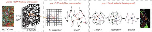
In this section, we designed a graph inductive learning model for hyperspectral remote sensing image classification, as shown in Figure 1. This method is mainly composed of three modules: LBP texture feature extraction module of hyperspectral images, K-nearest neighbor composition module and graph inductive learning module. These key steps are detailed in the sections below.

Figure 1. Flowchart of the proposed method

Graph inductive learning model

Transductive learning methods such as GCN often require all graph nodes to appear during training and can only generate unique embedded features for each node. On the contrary, graph inductive learning greatly improves the training efficiency by learning to generate aggregate functions with embedded features. As shown in the part 3 of Figure 1, the operation process of inductive learning in this paper is mainly divided into three steps:

• Sampling: Randomly sample the neighbors of each training node in the graph. For the sake of computational efficiency, $N$ neighbor nodes are sampled in each layer. If the number of neighbors of the node is less than $N$, the replacement sampling method will be adopted until $N$vertices are collected. If the number of vertex neighbors is greater than $N$, sampling without a replacement will be used.

• Aggregation: Aggregate the information contained in the sampled neighbor nodes according to the mean aggregation function. That means, the aggregated neighbor features will be fused with the features of the upper layer of the center node, and then the obtained features will be averaged element by element.

• Prediction: The aggregate information is input into the fully connected layer to obtain a new vector representation of each vertex in the graph, and finally the probability distribution of each node’s predicted label is obtained through the softmax function.

The forward propagation process of the proposed method is described as algorithm 1.

Table

Algorithm 1 Forward Propagation process of the graph inductive learning

Input:Graph $g(V,\xi )$; input feature $x_v,\mathrm{\forall }v\in V$; depth $L$; weight matrices $W^l,\mathrm{\forall }l\in (1,\cdot \cdot \cdot ,L)$; non-linearity $\sigma$; neighborhood function $N:v\to 2^V$

Output:Vector representations $z_v$ for $v\in V$ 1: $h_v^0\leftarrow x_v,\mathrm{\forall }v\in V$ 2: for $l=1\cdot \cdot \cdot L$ do 3: for $v\in V$do 4: $h_{N(v)}^l\leftarrow MEAN\{(h_v^{l-1})\cup (h_u^{l-1},\mathrm{\forall }u\in N_{(v)})\}$ 5: $h_v^l\leftarrow \sigma (W^l\cdot h_{N(v)}^l)$ 6: $h_v^l\leftarrow h_v^l/{∥h_v^l∥}_2,\mathrm{\forall }v\in V$ end for 7: $z_v\leftarrow h_v^l,\mathrm{\forall }v\in V$

end for

where $g(V,\xi )$ represents an undirected graph. $x_v$ represents the input vector of node $v$. $L$ is the number of layers of the model, representing the number of hops of adjacent nodes sampled and aggregated by each central node. For example, $L=2$ in the part 3 of Figure 1. $N(v)$ represents the sampled neighbor nodes of the central node $v$. $h_{N(v)}^l$ represents the characteristic representation of all neighbor nodes of node $v$ at layer $L$. The 4th and 5th lines of algorithm 1 indicate that the $L-1$ layer vector of the central node and sampled neighbor nodes is connected together, and then the mean value of each dimension of the vector is calculated. Finally, a nonlinear transformation is performed on the obtained results to generate the $L$ layer representation vector of the central node. $z_v$ is the output vector for each central node. In the training process, the cross-entropy loss is chosen as the loss function.

K-nearest neighbor construction

Since the graph inductive learning method can be only directly applied to graph structure data, it is necessary to construct HSI as graph. We treat each pixel of the HSI as a node of the graph, so that the HSI can be regarded as a matrix $X\in R^{N\times C}$, with $N$ is the number of samples, and $C$ is the dimension of the feature vector. We can calculate the euclidean distance between any two samples $x_i$ and $x_j$ according to Equation (1)(1) $d_{ij}=\sqrt{\sum _{c=1}^C{\left|x_{ic}-x_{jc}\right|}^2}$(1) :

(1) $d_{ij}=\sqrt{\sum _{c=1}^C{\left|x_{ic}-x_{jc}\right|}^2}$(1)

where $d_{ij}$ represents the distance between the $i$th pixel and the$j$th pixel. In order to construct HSI into a graph, we select the $K$ pixel points closest to pixel $x_i$ as neighbor nodes, and record the connection relationship between nodes with adjacency matrix $A\in R^{N\times N}$. Consequently, the HSI is constructed into a graph $g(V,\xi )$ with each pixel has $K$ connected neighbor nodes. $V$ and $\xi$ are the sets of nodes and edges.

Local binary patterns

In order to further improve the image classification accuracy, local binary patterns (LBP) are used to extract the spatial texture features of the image. LBP is an operator used to describe local texture features of an image, it has the advantages of simple principle, low computational complexity, rotation invariance and gray invariance. To extract the LBP texture of the image, the value of the central pixel is compared with the surrounding 8 neighborhood pixels to obtain the binary encoding of the 8 neighborhood pixels, and then the binary encoding is multiplied by the weight of the corresponding pixel. Finally, the weighted values of adjacent pixels are summed to obtain the LBP encoding representing the texture information of the center pixel. Figure 2 illustrates the flow of extracting texture using LBP.

Figure 2. The flow of extracting texture by LBP

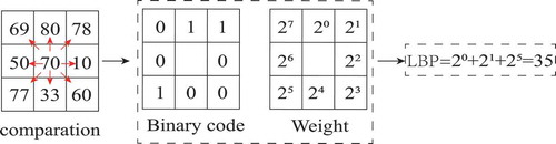
For HSI with hundreds of bands, PCA was first used to reduce the dimensions of HSI to three bands, and then LBP features are extracted from the three principal components, respectively. Finally, a six-dimensional feature vector is generated for each pixel of the image by combining the three principal component features with the three LBP features. The final extracted features include the main spectral features and texture features extracted by LBP, and the spatial-spectral information of hyperspectral images is also used.

Experiment and analysis

The proposed method is implemented by the PyTorch library. All experiments are generated on a PC equipped with an Intel Core i7-9750 H, 2.60 GHz and an Nvidia GeForce GTX 2070. The PC’s memory is 16 GB.

Experimental datasets

Our experiment results are conducted on three well-known HSI data sets including the University of Pavia (UP), the Salinas (SA) and the Pavia Center (PC). To demonstrate the classification power of the proposed method under the conditions of small sample, 5,10,15 labeled samples per class are selected successively as training samples, and the whole samples of each images are selected as testing samples to conduct experiments. Moreover, in order to compare and analyze the experiment results quantitatively, overall accuracy(OA) is adopted as the metric.

The University of Pavia data set is acquired by the ROSIS sensor during a flight campaign over Pavia, northern Italy. It has 103 spectral band coverage from 0.43 to 0.86 µm and a geometric resolution of 1:3 m. The image size is 610 × 340 pixels. In this data set, 42,776 pixels with nine classes are labeled. The Class name, number of labeled training samples, number of testing samples are listed in Table 1.

Table 1. Class name, number of training samples, number of testing samples for the University of Pavia data set

	Class	Training	Testing
1	Asphalt	5/10/15	6631
2	Meadows	5/10/15	18649
3	Gravel	5/10/15	2099
4	Trees	5/10/15	3064
5	Sheets	5/10/15	1345
6	Bare Soil	5/10/15	5029
7	Bitumen	5/10/15	1330
8	Bricks	5/10/15	3682
9	Shadows	5/10/15	947
Total		45/90/135	42776

Salinas data set is gathered by the AVIRIS sensor in north-west Indian. There are 224 spectral channels range from 0.4 to 2.5 µm with a spatial resolution of 3.7 m. The area covered comprises 512 × 217 pixels. As with the Indian Pines data set, 20 water absorption bands are discarded. A total of 54129 pixels with 16 classes are labeled. The Class name, number of labeled training samples, number of testing samples are listed in Table 2.

Table 2. Class name, number of training samples, number of testing samples for the Salinas data set

No.	Class	Training	Testing
1	Brocoli_green_weeds_1	5/10/15	2009
2	Brocoli_green_weeds_2	5/10/15	3726
3	Fallow	5/10/15	1976
4	Fallow_rough_plow	5/10/15	1394
5	Fallow_smooth	5/10/15	2678
6	Stubble	5/10/15	3959
7	Celery	5/10/15	3579
8	Grapes_untrained	5/10/15	11271
9	Soil_vinyard_develop	5/10/15	6203
10	Corn_senesced_green_weeds	5/10/15	3278
11	Lettuce_romaine_4 wk	5/10/15	1068
12	Lettuce_romaine_5 wk	5/10/15	1927
13	Lettuce_romaine_6 wk	5/10/15	916
14	Lettuce_romaine_7 wk	5/10/15	1070
15	Vinyard_untrained	5/10/15	7268
16	Vinyard_vertical_trellis	5/10/15	1807
Total		80/160/240	54129

Pavia center data set is gathered by the AVIRIS sensor in Italy Pavia center. There are 102 spectral channels range from 0.43 to 0.86 µm with a spatial resolution of 1.3 m. The area covered comprises 1096 × 715 pixels. In this data set, 148152 pixels with nine classes are labeled. The Class name, number of labeled training samples, number of testing samples are listed in Table 3.

Table 3. Class name, number of training samples, number of testing samples for the Pavia center data set

No.	Class	Training	Testing
1	Water	5/10/15	65971
2	Trees	5/10/15	7598
3	Meadow	5/10/15	3090
4	Brick	5/10/15	2685
5	Bare Soil	5/10/15	6584
6	Asphalt	5/10/15	9248
7	Bitumen	5/10/15	7287
8	Tile	5/10/15	42826
9	Shadows	5/10/15	2863
Total		45/90/135	148152

Experimental settings

In the process of graph construction, the value of parameter K represents the number of neighbor nodes of each node. In the process of sampling, $N$ nodes are randomly sampled from $K$ neighbor nodes as the information nodes to be aggregated. In order to determine the optimal parameters $N$ and $K$, we conducted classification experiments on three data sets under different $K$ values (10, 20, 30) and different $N$ values (5, 10, 15, 20, 25, 30) to record the overall accuracy and the training time. As is shown in Tables 4Tables 5–6, the different combinations of $K$ and $N$ have a greater impact on the experimental results. When $N$ is fixed, as the $K$ value becomes larger, the overall accuracy basically shows a trend that first becomes larger and then becomes smaller, while the training time does not change much. When the value of $K$ is fixed, as the value of $N$ increases, the training time increases more obviously, but the overall classification accuracy is not very sensitive to changes in the value of $N$. Comprehensive consideration of training time and classification accuracy. In the end, the $K$ value of Pavia University is 30 and $N$ is 5, the $K$ value of Salinas is 20 and $N$ is 5, the $K$ value of Pavia Center is 20 and $N$ is 5.

Table 4. Overall accuracy and training time of the Pavia university data set (UP) under the combination of different neighbor number ($K$) and sample number ($N$)

Sample number (N)	Neighbor number (K)
	10		20		30
	Acc	Time	Acc	Time	Acc	Time
5	73.78	1005.6	74.1	1154.9	76.52	1205.3
10	71.52	1482.2	72.02	1553.3	73.58	1609.8
15	73.3	1576.4	73.76	1629.7	73.84	1709.6
20	70.05	1846.7	72.01	1892.8	73.48	1946.9
25	73.29	2006.9	74.05	2093.7	74.09	2112.8
30	73.37	2475.4	73.75	2506	74.14	2588.6

Table 5. Overall accuracy and training time of the Salinas data set (SA) under the combination of different neighbor number ($K$) and sample number ($N$)

Sample number (N)	Neighbor number (K)
	10		20		30
	Acc	Time	Acc	Time	Acc	Time
5	80.99	2433.6	82.43	2501.8	81.25	2593.5
10	80.81	2976.1	81.24	3035	81.2	3128.6
15	80.79	3129.4	81.08	3128.6	81.19	3229.4
20	80.71	3288.2	81.22	3326.2	81.16	3406.7
25	80.69	3574.6	81.34	3633.7	81.26	3763.4
30	80.99	3864.9	81.37	3927.4	81.34	4005.9

Table 6. Overall accuracy and training time of the Pavia Center data set (PC) under the combination of different neighbor number ($K$) and sample number ($N$)

Sample number (N)	Neighbor number (K)
	10		20		30
	Acc	Time	Acc	Time	Acc	Time
5	95.21	4058.5	95.91	4106.3	95.35	4230.5
10	95.33	4831	95.77	4951.4	95.37	5004.6
15	94.26	5127.6	94.88	5281.4	94.63	5409.8
20	94.27	5644.9	94.81	5781.6	94.74	5891.6
25	95.31	5951.8	95.5	6118.5	94.95	6237.9
30	94.52	6334.8	95.09	6471.9	94.73	6582.7

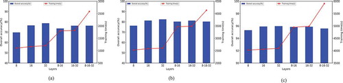
In the aggregation process, the number of neighbor layers traversed by the central node will determine the training time cost and the quality of the aggregated information, which will affect the final classification performance. In order to discuss the best layer settings in detail, we analyzed the overall accuracy and training time in the case of combining the output dimensions of each layer. As shown in Figure 3, the X axis represents different layer settings. For example, 8–16 means that the central node aggregates sampling neighbor nodes in two layers. The feature dimension of the output of the first layer is 8, and the feature dimension of the output of the second layer is 16. In addition, the blue bar chart and the red line represent the overall classification accuracy and training time, respectively. It can be found that when the number of layers is the same, the overall accuracy will increase with the increase of output dimension, and the training time will not change significantly. As the number of layers increases, the training time increases greatly and the classification accuracy decreases. Therefore, it was finally determined that the central node aggregated the sampled neighbor information of one layer and the output dimension was 32.

Figure 3. The classification accuracy and the training time under different layers. (a) University of Pavia data set, (b) Salinas data set and (c) Pavia Center data set

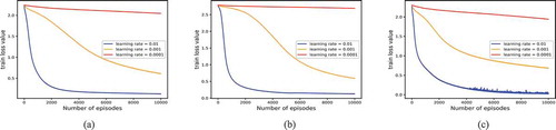
Finally, we set the number of training iterations to 10,000 and optimized the training process with SGD optimizer. During the training, we recorded the changes of the loss function value corresponding to different learning rates (e.g. 0.01, 0.001, 0.0001) and plotted its change curve. As shown in Figure 4, it can be found that a small learning rate (e.g. 0.001, 0.0001) is not conducive to the training process and will lead to a large loss of function value. In contrast, a small learning rate (e.g. 0.01) could decrease the train loss value. Therefore, the learning rate is set to 0.01.

Figure 4. The training loss values with different learning rates. (a) University of Pavia data set, (b) Salinas data set and (c) Pavia Center data set

Classification results and analysis

To evaluate the classification capability of our proposed method (Abbreviation as LBP+Graphsage), other hyperspectral image classification methods are used for comparison. Specifically, we employ the traditional support vector machine (SVM), five traditional semi-supervised algorithms (Wang et al., 2014) including the Laplacian Support Vector Machine (LapSVM), the Transductive Support Vector Machine (TSVM), the Spatial-Contextual SemiSupervised Support Vector Machine (SCS³VM). Two advanced deep learning method Res-3D-CNN (Bing Liu, Yu, Zhang, Tan et al., 2018) and the semi-supervised deep learning model SS-CNN (Liu et al., 2018). In addition, we also used the original spectral features (Graphsage for short) for classification to verify the effectiveness of LBP in extracting spatial features. All of these methods were executed 10 times on each dataset. The average accuracy and standard deviation of these 10 independent implementations are reported in Tables 7Tables 8–9, where $L$ represents the number of samples randomly selected from each type of ground objects.

Table 7. Overall accuracy (%) of the different methods for the UP data set

Method	L = 5	L = 10	L = 15
SVM	53.73 ± 1.30	61.53 ± 1.14	60.43 ± 0.94
LapSVM	65.72 ± 0.34	68.26 ± 2.20	68.34 ± 0.29
TSVM	63.43 ± 1.22	63.73 ± 0.45	68.45 ± 1.07
SCS^3VM	56.76 ± 2.28	64.25 ± 0.40	66.87 ± 0.37
Res-3D-CNN	65.44 ± 2.14	66.89 ± 2.07	68.12 ± 1.56
SS-CNN	71.73 ± 2.38	72.15 ± 2.09	74.56 ± 1.05
Graphsage	64.39 ± 0.64	69.67 ± 0.58	71.19 ± 0.55
LBP+Graphsage	77.87 ± 0.31	79.54 ± 0.42	81.20 ± 0.41

Table 8. Overall accuracy (%) of the different methods for the SA data set

Method	L = 5	L = 10	L = 15
SVM	73.90 ± 1.91	75.62 ± 1.73	79.08 ± 1.45
LapSVM	75.31 ± 2.31	76.34 ± 1.77	77.93 ± 2.42
TSVM	60.43 ± 1.40	67.47 ± 1.05	69.12 ± 1.32
SCS^3VM	74.12 ± 2.44	78.49 ± 2.02	81.83 ± 0.93
Res-3D-CNN	67.60 ± 1.89	69.12 ± 1.53	73.22 ± 1.17
SS-CNN	79.23 ± 2.06	80.15 ± 1.23	81.06 ± 0.94
Graphsage	79.44 ± 1.01	80.24 ± 0.95	81.00 ± 0.73
LBP+Graphsage	82.70 ± 0.95	83.89 ± 0.71	85.22 ± 0.68

Table 9. Overall accuracy (%) of the different methods for the PC data set

Method	L = 5	L = 10	L = 15
SVM	79.51 ± 0.64	89.33 ± 0.28	90.88 ± 1.72
LapSVM	88.03 ± 0.80	89.91 ± 0.97	91.66 ± 0.40
TSVM	68.00 ± 0.56	67.89 ± 0.69	72.94 ± 0.63
SCS^3VM	91.24 ± 0.70	91.72 ± 0.38	93.68 ± 1.00
Res-3D-CNN	80.03 ± 1.20	84.36 ± 0.98	86.56 ± 0.79
SS-CNN	89.27 ± 1.66	90.68 ± 1.39	92.35 ± 0.99
Graphsage	95.38 ± 0.94	96.19 ± 0.81	96.79 ± 0.53
LBP+Graphsage	95.97 ± 0.59	96.87 ± 0.37	97.61 ± 0.31

From these results, we can learn that overall accuracy of all algorithms rises with the increase of the number of training samples, which indicates that increasing the number of training samples can improve the generalization ability of the model and thus improve the classification accuracy of HSI. Compared with the traditional supervised classifier SVM, the traditional semi-supervised algorithm (e.g. LapSVM, TSVM and SCS³VM) can achieve higher classification accuracy by utilizing both labeled samples and unlabeled samples. The deep learning method Res-3D-CNN is easy to overfit in the case of small samples, so the classification performance is poor. SS-CNN combines the CNN model with semi-supervised learning, so the overall accuracy is better than Res-3D-CNN. The methods of graph neural networks (e.g. Graphsage, LBP+Graphsage) classify the HSI based on the graph nodes and can characterize the irregular local area of the HSI. Therefore, the classification accuracy is relatively high under the conditions of small samples. The proposed method (LBP+Graphsage) achieves the highest classification accuracy and the lowest variance on the Pavia University data set, which indicates the effectiveness of this method for HSI classification under the conditions of small samples. In addition, the classification accuracy of LBP+Graphsage is higher than that of Graphsage, indicating that the spatial features extracted by LBP are conducive to improving the classification accuracy.

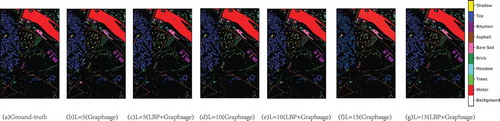
In order to more specifically observe the classification results of LBP+Graphsage and Graphsage, Figures 5–7 show the classification maps of the three data sets. It can be found that classification noise decreases gradually with the increase of L, and LBP can effectively reduce classification noise under the same labeled sample conditions.

Figure 5. The classification maps from the proposed method in the UP data set

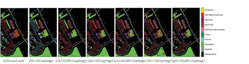
Figure 6. The classification maps from the proposed method in the SA data set

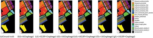
Figure 7. The classification maps from the proposed method in the PC data set

To further analyze the execution time of the proposed method, in this section, LapSVM and SS-CNN whose classification accuracy was close to LBP+Graphsage were selected as comparison algorithms. As is shown in Table 10, the execution time includes the training time and the test time. For the traditional semi-supervised algorithm, LapSVM has fewer super parameters, so the training time is very short. However, the classification accuracy of LapSVM is low. Due to the large scale of hyperspectral images after composition, the training time of LBP+Graphsage was relatively large, which was basically equivalent to SS-CNN. But the classification accuracy of LBP+Graphsge is higher than that of SS-CNN. In addition, Table 11 shows the number of parameters of three different deep learning models on the Pavia university data set. It can be seen that GraphSage has fewer model parameters than Res-3D-CNN and SS-CNN.

Table 10. Execution times on three target data set (five samples per class are used as training samples)

Data set	LapSVM	SS-CNN	LBP+Graphsage
UP	10.56(s)+0.10(s)	1220.21(s)+1.64(s)	1205.31(s)+0.04(s)
SA	12.38(s)+0.34(s)	1465.33(s)+5.62(s)	2501.91(s)+0.06(s)
PC	29.63(s)+0.21(s)	2564.42(s)+2.34(s)	4106.31(s)+1.82(s)

Table 11. Number of model parameters of different models on the Pavia University data set

Res-3D-CNN	SS-CNN	Graphsage
60370130	26230120	1155528

Conclusion

In this paper, we designed a graph inductive learning method for small sample classification of HSI. Based on LBP texture feature extraction and K-nearest neighbor construction, this method learns the aggregation mode between graph nodes by sampling and aggregation operation. Experimental results on three typical data sets demonstrate the effectiveness of the proposed method. However, the large number of nodes in hyperspectral images will lead to low computational efficiency. The next step is to consider using superpixels as vertices in the graph to reduce computational costs.

Acknowledgments

We would like to thank Prof. WilliamL. Hamilton for providing their method of Graphsage.

Disclosure statement

No potential conflict of interest was reported by the authors.

Additional information

Funding

This research was funded by the National Natural Science Foundation of China [41801388].

References

- Achanta, R., Shaji, A., Smith, K., Lucchi, A., Fua, P., & Süsstrunk, S., & Analysis, S. S. s. J. I. T. o. P., & Intelligence, M. (2012). SLIC superpixels compared to state-of-the-art superpixel methods. IEEE Transactions on Pattern Analysis and Machine Intelligence, 34(11), 2274–2282. https://doi.org/10.1109/TPAMI.2012.120
- Bai, Y., Zhang, Q., Lu, Z., & Zhang, Y. J. I. A. (2019). SSDC-DenseNet: A cost-effective end-to-end spectral-spatial dual-channel dense network for hyperspectral image classification. IEEE Access,(99), 1. https://doi.org/10.1109/ACCESS.2019.2925283
- Chen, Y., Jiang, H., Li, C., Jia, X., & Ghamisi, P. J. I., T. o. G., & Sensing, R. (2016). Deep feature extraction and classification of hyperspectral images based on convolutional neural networks. IEEE Transactions on Geoscience and Remote Sensing, 54(10), 6232–6251. https://doi.org/10.1109/TGRS.2016.2584107
- Chen, Y., Lin, Z., Zhao, X., Wang, G., & Gu, Y. J. I., & J. o. S. T. i. A. E. O., & Sensing, R. (2014). Deep learning-based classification of hyperspectral data. ChemSusChem, 7(6), 2094–2107. https://doi.org/10.1002/cssc.201402220
- Fang, S., Quan, D., Wang, S., Zhang, L., & Zhou, L. (2018). A two-branch network with semi-supervised learning for hyperspectral classification.IEEE international geoscience and remote sensing symposium.
- Gao, K., Guo, W., Yu, X., Bing, L., & Wei, X. J. I., J. o. S. T. i. A. E. O., & Sensing, R. (2020). Deep induction network for small samples classification of hyperspectral images. IEEE Journal of Selected Topics in Applied Earth Observations and Remote Sensing,(99), 1. https://doi.org/10.1109/JSTARS.2020.3002787
- Ghamisi, P., Dalla Mura, M., & Benediktsson, J. A. J. I., T. o. G., & Sensing, R. (2015). A survey on spectral&spatial classification techniques based on attribute profiles. IEEE Transactions on Geoscience and Remote Sensing,53(5), 2335–2353. https://doi.org/10.1109/TGRS.2014.2358934
- Ghamisi, P., Plaza, J., Chen, Y., Li, J., Plaza, A. J. J. G., & Sensing, R. (2017). Advanced spectral classifiers for hyperspectral images: A review. IEEE Geoscience and Remote Sensing Magazine,5(1), 8–32.https://doi.org/10.1109/MGRS.2016.2616418
- Hamilton, W. L., Ying, Z., & Leskovec, J. (2017). Inductive representation learning on large graphs. http://papers.nips.cc/paper/6703-inductive-representation-learning-on-large-graphs
- Hong, D., Gao, L., Yao, J., Zhang, B., Plaza, A., & Chanussot, J. (2020). Graph convolutional networks for hyperspectral image classification. IEEE Transactions on Geoscience and Remote Sensing, 1–13. https://doi.org/10.1109/TGRS.2020.3015157
- Hong, D., Yokoya, N., Chanussot, J., & Zhu, X. X. (2019). An augmented linear mixing model to address spectral variability for hyperspectral unmixing. IEEE Transactions on Image Processing, 28(4), 1923–1938. https://doi.org/10.1109/TIP.2018.2878958
- Jihao, Y., Sen, L., Hongmei, Z., & Xiaoyan, Geoscience, L. J., & Remote Sensing Letters, I. (2019). Hyperspectral image classification using CapsNet with well-initialized shallow layers. IEEE Geoscience and Remote Sensing Letters,16(7), 1095–1099. https://doi.org/10.1109/LGRS.2019.2891076
- Kipf, T. N., & Welling, M. (2016). Semi-Supervised Classification with Graph Convolutional Networks.
- Li, S., Song, W., Fang, L., Chen, Y., Ghamisi, P., & Benediktsson, J. A. (2019). Deep learning for hyperspectral image classification: An overview. IEEE Transactions on Geoscience and Remote Sensing, 57(9), 6690–6709. https://doi.org/10.1109/TGRS.2019.2907932
- Li, W., Chen, C., Su, H., & Du, Q. J. I., T. o. G., & Sensing, R. (2015). Local binary patterns and extreme learning machine for hyperspectral imagery classification. IEEE Transactions on Geoscience and Remote Sensing,53(7), 3681–3693. https://doi.org/10.1109/TGRS.2014.2381602
- Liu, B., Yu, A., Yu, X., Wang, R., & Guo, W. J. I., T. o. G., & Sensing, R. (2020). Deep multiview learning for hyperspectral image classification. IEEE Transactions on Geoscience and Remote Sensing,(99), 1–15. https://doi.org/10.1109/TGRS.2020.3034133
- Liu, B., Yu, X., Yu, A., Zhang, P., Wan, G., & Wang, R. (2019). Deep few-shot learning for hyperspectral image classification. IEEE Transactions on Geoscience and Remote Sensing, 57(4), 2290–2304. https://doi.org/10.1109/TGRS.2018.2872830
- Liu, B., Yu, X., Yu, A., Zhang, P., & Wan, G. J. R. S. L. (2018). Spectral-spatial classification of hyperspectral imagery based on recurrent neural networks. Remote Sensing Letters, 9(10–12), 1118–1127. https://doi.org/10.1080/2150704X.2018.1511933
- Liu, B., Yu, X., Zhang, P., Tan, X., Wang, R., & Zhi, L. (2018). Spectral–spatial classification of hyperspectral image using three-dimensional convolution network. Journal of Applied Remote Sensing, 12(1), 016005. https://doi.org/10.1117/1.JRS.12.016005
- Liu, B., Yu, X., Zhang, P., Tan, X., Yu, A., & Xue, Z. (2017). A semi-supervised convolutional neural network for hyperspectral image classification. Remote Sensing Letters, 8(9), 839–848. https://doi.org/10.1080/2150704X.2017.1331053
- Liu, B., Yu, X., Zhang, P., Yu, A., Fu, Q., & Wei, X. (2018). Supervised deep feature extraction for hyperspectral image classification. IEEE Transactions on Geoscience and Remote Sensing, 56(4), 1909–1921. https://doi.org/10.1109/TGRS.2017.2769673
- Ma, X., Mou, X., Wang, J., Liu, X., Wang, H., & Yin, B. J. I., T. o. G., & Sensing, R. (2019). Cross-data set hyperspectral image classification based on deep domain adaptation. IEEE Transactions on Geoscience and Remote Sensing,57(12), 10164–10174. https://doi.org/10.1109/TGRS.2019.2931730
- Mei, S., Ji, J., Geng, Y., Zhang, Z., Li, X., & Du, Q. J. I., T. o. G., & Sensing, R. (2019). Unsupervised spatial–spectral feature learning by 3D convolutional autoencoder for hyperspectral classification. IEEE Transactions on Geoscience and Remote Sensing,57(9), 6808–6820. https://doi.org/10.1109/TGRS.2019.2908756
- Palmason, J. A., Benediktsson, J. A., Sveinsson, J. R., & Chanussot, J. (2005). Classification of hyperspectral data from urban areas using morphological preprocessing and independent component analysis. IEEE international geoscience & remote sensing symposium.
- Qin, A., Shang, Z., Tian, J., Wang, Y., Zhang, T., Tang, Y. Y. J. I. G., & Letters, R. S. (2018). Spectral–spatial graph convolutional networks for semisupervised hyperspectral image classification. IEEE Geoscience and Remote Sensing Letters, (2), 1–5. https://doi.org/10.1109/LGRS.2018.2869563
- Scarselli, F., Gori, M., Tsoi, A. C., Hagenbuchner, M., & Monfardini, G. J. I. T. O. N. N. (2009). The graph neural network model. IEEE Transactions on Neural Networks, 20(1), 61.https://doi.org/10.1109/TNN.2008.2005605
- Sheng, W., Chen, G., Ping, Z., Du, B., Lefei, G., Lu, C., & Xu, -J.-J., & Z. J. I. T. o., & Sensing, R. (2019). Multiscale dynamic graph convolutional network for hyperspectral image classification. Angewandte Chemie (International Ed. In English), 58(5), 3162–3177. https://doi.org/10.1002/anie.201900283
- Wang, L., Hao, S., Wang, Q., & Wang, Y. J. I., J. o. P., & Sensing, R. (2014). Semi-supervised classification for hyperspectral imagery based on spatial-spectral Label Propagation. ISPRS Journal of Photogrammetry and Remote Sensing, 97, 123–137. https://doi.org/10.1016/j.isprsjprs.2014.08.016
- Yue, J., Zhao, W., Mao, S., & Liu, H. J. R. S. L. (2015). Spectral–spatial classification of hyperspectral images using deep convolutional neural networks. Remote Sensing Letters, 6(4–6), 468–477. https://doi.org/10.1080/2150704X.2015.1047045