A multi-scale multi-channel CNN introducing a channel-spatial attention mechanism hyperspectral remote sensing image classification method

ABSTRACT

Aiming the problems that the classification performance of hyperspectral images in existing classification algorithms is highly dependent on spatial-spectral information and that detailed features are ignored in single convolutional channel feature extraction, resulting in poor generalization performance of the feature extraction model, a multi-scale multi-channel convolutional neural network (MMC-CNN) model is proposed in this paper. First, the data set is divided into two kinds of pixel module, and then different channels are used for feature extraction. A channel-space attention mechanism module is also introduced, and a multi-scale multichannel convolutional neural network (CSAM-MMC) model with the introduction of channel-space attention mechanism is proposed for deeper spatial-spectral feature extraction of hyperspectral image elements while reducing the redundancy of convolutional pooling parameters to achieve better HSI classification. To evaluate the effectiveness of the proposed model, experiments were conducted on Indian Pines, Pavia Center and KSC datasets respectively, and the overall classification accuracies of this paper’s MMC-CNN model in the HSI dataset were 97.23%, 98.50%, and 97.85%, thus verifying the model’s high feature extraction accuracy. The CSAM-MMC model in this paper further improves 0.13%, 0.35%, and 0.71% relative to the MMC-CNN model, which provides higher overall accuracies relative to other state-of-the-art algorithms.

KEYWORDS:

• Hyperspectral images
• pixel module
• multi-scale multi-channel
• convolutional neural network
• spatial–spectral feature extraction

Introduction

The development of hyperspectral remote sensing images is an important milestone for the modern field of remote sensing, which contains rich feature information in hundreds of continuous spectral bands with high resolution, even to the nanometer level (Roy, Mondal, et al., 2021). Continuous spectral values can distinguish many different objects and provide valuable information for identifying various materials (Du et al., 2013). Hyperspectral images can simultaneously acquire spatial-spectral information by carrying different space platform sensors. Compared with ordinary remote sensing images, they have more two-dimensional image spatial information and one-dimensional spectral information describing the distribution of ground objects. Hyperspectral images are widely used in various fields, such as precision agriculture (Gevaert et al., 2015), environmental monitoring (Awad, 2014; Fakhrullin et al., 2021), military surveillance (Pi et al., 2021), and many other applications. In hyperspectral image processing, HSI classification is realized by different HSI pixel types (Zahisham et al., 2023), among which object classification is one of the important research directions of HSI. Rich ground feature information has a leading edge in ground feature classification.

Hyperspectral remote sensing image classification usually consists of two main parts, feature extraction as well as classification. Feature extraction is an essential and important part of the remote sensing image classification process, which can reduce the number of participating feature images on the one hand and better extract feature images for classification from the original information on the other hand. The purpose of feature extraction is to map from high-dimensional space to low-dimensional space, and then to classify different features according to the features of different features. The methods of feature extraction contain linear and nonlinear, which include: linear discriminant analysis (LDA) (Lu et al., 2023), independent component analysis (ICA) (Villa et al., 2011), principal component analysis (PCA) (Jiang et al., 2018) and local preserving projection (LPP) (Wang & He, 2011). After feature extraction, the obtained feature information is fed to the classifier for classification. Commonly used classifiers are Support Vector Machine (SVM) (Camps-Valls et al., 2006), Extreme Learning Machine (ELM) (W. Li et al., 2015), etc.

Deep learning methods are now widely used in many fields such as natural language processing (Young et al., 2017), speech recognition (H. Zhang et al., 2017), and computer vision (Voulodimos et al., 2018). When compared to traditional methods, it is able to automatically learn to automatically up-date the weight information by continuously optimizing the network parameters.

In recent years, with the development of deep learning (DL), many DL-based classification methods have been employed for HSI, and the classification performance has been dramatically enhanced (Zheng et al., 2024). Chen et al. first introduced deep learning models to HSI classification (Y. Chen et al., 2014), and there are many deep learning-based HSI classification methods, including stacked autoencoders (SAEs), deep confidence networks (DBNs), convolutional neural networks (CNN), recurrent neural networks (RNN), residual networks, and generative adversarial networks (GAN). Paul and Kumar proposed an improved SAE algorithm by using mutual information (MI) to perform segmented spectra, compared with SAE’s feature extraction, building a piece of mutual information (MI) based segmented stacked autoencoder (S-SAE), such segmentation methods reduce complexity and computation time. The main problem of SAE lies in the spatial finite element stage, where image patches are flattened into vectors, resulting in the loss of spatial information (Y. Xu et al., 2018). They exploit spatial features while also destroying the initial spatial structure. In order to alleviate this problem, the CNN method is introduced into the HSI classification task, and the CNN-based method effectively reduces the number of parameters in the deep learning model. Making full use of channel correlation and layered complementarity, Zhai proposed an end-to-end one-dimensional convolutional neural network to construct an effective multi-level one-dimensional convolutional neural network, which can hierarchically mine local channel correlations and comprehensively utilize shallow layers. and deep features to further enhance the discriminability of features (Zhai et al., 2022). Traditional convolutional neural network (CNN)-based methods mainly use 1D-CNN for spectral feature extraction and 2D-CNN for spatial feature extraction, which makes the inter-band correlation of HSI underutilized, while hyperspectral image classification performance is highly dependent on spatial and spectral information. 3D-CNN extracts joint spectral-spatial information representation, but it relies on more complex models (Ghaderizadeh et al., 2021). Xu proposed a classification method based on class incremental learning, designing a knowledge extraction strategy that transfers knowledge to a newly trained network to recall information from old classes, along with a linear correction layer and the introduction of an attention mechanism (M. Xu et al., 2022). Firat et al. proposed a hybrid 3D residual space-spectrum convolutional network to overcome the problems of network degradation and gradient disappearance while extracting spatial spectral features (Firat et al., 2023). Xie et al. retained the SegFormer decoder and improved the Swin Transformer to replace the encoder in SegFormer. The hyperpatch embedding module is introduced for feature extraction, and a transposed filling upsampling module for model output is proposed to realize end-to-end hyperspectral image classification (Xie et al., 2023).

In addition, for the existing deep learning classification method network structure, some detailed features will be ignored during the feature extraction of a single convolution channel, and the generalization performance of the feature extraction model is poor. Multichannel and multi-scale feature fusion methods are very attractive for HSI classification. Researchers use two or more channels to extract features and finally input the fused feature maps together for classification to better express the spatial and spectral information of ground objects. In multi-scale, use convolution kernels of different sizes to extract HSI features, and then fuse them together for final result classification; another case is to crop three-dimensional pixel modules of different sizes in the input feature layer, input into the model for predictive classification. Yang et al. adopted a dual-channel network framework to jointly learn spectral-spatial features of hyper-spectral images. Each channel is concatenated from features learned from spectral and spatial domains respectively and fed to a fully connected layer for extracting joint spectral-spatial features. In the case of a small number of training samples, based on multi-channel feature extraction and feature fusion, Pei proposes a simple and efficient two-channel spectral enhancement network, which makes full use of the features of small samples with labels for HSI classification (Pei et al., 2022). Bei et al. used a multi-channel lightweight integration framework, frequency band clustering, and selection strategies to train different training samples in different bands. After every single network was trained, a weighted voting strategy was used to make combined decisions on the generated classification sets (Fang et al., 2021). In order to solve the insufficient training samples, Dong et al. proposed a deep integrated CNN method based on sample expansion for HSI classification (Dong et al., 2022). Zhang et al. used a dual-channel convolutional neural network framework. The first channel used 1D-CNN to extract spectral feature information; the second channel used 2D-CNN to extract spatial feature information, and finally the two channels extracted information to jointly output classification results (H. Zhang et al., 2017b). Both 1D-CNN and 2D-CNN will compress the original image, destroying the characteristic information of the original 3D image. In order to avoid the drawbacks of traditional classification models that only focus on one-dimensional feature extraction. On this basis, Li et al. introduced 3D-CNN to the dual-branch residual neural network and designed a training method for self-supervised classification tasks according to the characteristics of HSI (T. Li et al., 2022). Asker is trained using a three-branch network structure, with the first branch using a squeezing and excitation network, the second branch using a hybrid 3D-CNN and 2D-DSC method, and the third branch using a 2D-DSC method alone to further extract features from the HSI (Asker, 2023). It also laid the foundation for the use of 3D-CNN in this paper. In the process of hyperspectral data processing, it is not enough to select some specific bands, and more importantly, to obtain the correlation between the data spatial distribution rules and spectral features hidden in the original data. All of the above methods obtain feature information for a hyperspectral image of a specific size. The correlation between spectral information and spatial information is not fully utilized, resulting in the loss of some detailed features, and there will be a large number of parameters, which is prone to overfitting. Therefore, this paper designs hyperspectral pixel modules with two scales, which doubles the efficiency. At the same time, 3D-CNN is used to directly extract feature information, fully considering the complementary information and correlation in the two-dimensional spatial domain and the one-dimensional spectral domain.

In order to improve the performance of the model for feature extraction and make better use of the relationship between channels and spatial positions, Woo et al. incorporated a CBAM module into the base CNN model, which is a combination of a channel attention mechanism module and a spatial attention mechanism module to weight spectral and spatial processing to effectively capture image features (Woo et al., 2018). Li et al. applied a channel attention block and a spatial attention block to a dual-branch network structure, enabling refinement and optimization of the extracted feature maps (R. Li et al., 2020). Qing et al. fused the multiscale residual convolutional neural network model with the attention mechanism network to further improve the accuracy of deep learning classification (Qing & Liu, 2021). Ren et al. assisted CNNs to learn classification by employing an attention module to fully explore the prior information of different spectral bands and spatial locations in a hyperspectral cube (Hang et al., 2021). In the case of limited samples, Shi et al. proposed a three-dimensional coordinated attention mechanism to obtain the long-distance dependence of the spatial position of HSI in the vertical and horizontal directions, so as to obtain the difference between different spectral bands and achieve comprehensive extraction of spectral-spatial information (Shi et al., 2022). Therefore, this paper combines the multi-scale multi-channel convolutional neural network and the spatial-spectral attention mechanism module to effectively integrate the channel and spatial dimensions of the feature map.

All the above methods can be used to sort hyperspectral images, but since the typical CNN network uses a single patch structure to indicate the samples to be sorted, it can contribute to classification errors in irregular regions. Furthermore, the simple network structure extracts limited features and thus the classification accuracy needs to be improved. The principal contribution of this paper is a multi-scale multichannel CNN that introduces a channel-space attention mechanism module to implement a hyperspectral image classification framework, which makes full use of the multichannel network structure by changing the network structure and adjusting the hyperparameters to process multiple input data of different sizes for deeper feature extraction and more effectively address the few categories with low classification accuracy.

1. In the data set processing, the original data set is cut into pixel modules of two different scales to obtain the characteristic information of the hyperspectral pixel module;

2. In this paper, a multi-scale multi-channel convolutional neural network (MMC-CNN) model is proposed. At first, the data set is divided into two pre-defined scales $X_1\times X_1$ pixel module and $X_2\times X_2$ pixel module, and then two $X_1\times X_1$ module channels and two $X_2\times X_2$ module channels are adopted for feature extraction, and 3D convolutional kernels are used as feature extractors for each channel. Effectively solving the problem that single convolutional channel feature extraction will be ignored the relevant detailed features, resulting in poor generalization capability of the feature extraction model;

3. For the purpose of focusing more on spatial-spectral feature information, a channel-spatial attention mechanism module is introduced. In this paper, a multi-scale multichannel convolutional neural network (CSAM-MMC) model with the introduction of a channel-spatial attention mechanism is proposed for deeper spatial-spectral feature extraction of hyperspectral image elements, while reducing the redundancy of convolutional pooling parameters to accomplish an improved HSI classification;

4. We conduct experimental verification on three public datasets. By comparing our proposed network with other advanced methods, the results obtained show the effectiveness of the proposed method.

5. In the second section, the basic knowledge and principles are mainly introduced; in the third section, the MMC-CNN model and experimental results proposed in this paper will be introduced; in the fourth section, the CSAM-MMC model method and experimental results proposed in this paper will be introduced Results; the experiments of the model in this paper on three HSI data sets (Indian Pines, Pavia Center, KSC) compare the performance of the method in this paper; the conclusion of the fifth part summarizes the advantages and disadvantages of the model in this paper and the direction of further improvement.

In the second section, the basic knowledge and principles are mainly introduced; in the third section, the MMC-CNN model and experimental results proposed in this paper will be introduced; in the fourth section, the CSAM-MMC model method and experimental results proposed in this paper will be introduced Results; the experiments of the model in this paper on three HSI data sets (Indian Pines, Pavia Center, KSC) compare the performance of the method in this paper; the conclusion of the fifth part summarizes the advantages and disadvantages of the model in this paper and the direction of further improvement.

Materials

Convolutional neural networks

At present, convolutional neural networks (CNNs) have been widely used in image processing and pattern recognition (Feng et al., 2021). As compared with DBN and SAE, CNN has its unique advantages, such as image blocks are not flattened into vectors, spatial information is retained intact, and has a more powerful feature extraction capability, therefore CNN is the most commonly used deep learning model for hyperspectral image classification.

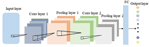
A classical convolutional neural network usually contains an input layer, a convolutional layer, an activation function, a pooling layer, a fully connected layer, and an output layer. A convolutional neural network model generally has several convolutional layers, pooling layers, and fully connected layers, however, each layer has its own unique function, where the convolutional, pooling, and fully connected layers are all the hidden layers in a CNN, and the basic structure of a CNN is shown in Figure 1.

Figure 1. Convolutional neural network structure.

There are three different types of convolution computing kernels in the current convolutional neural network: 1D-CNN, 2D-CNN, and 3D-CNN. Spectral information is a one-dimensional vector, which is usually classified using 1D-CNN. 2D-CNN can be used to extract local spatial information around target pixels in hyperspectral remote sensing images. The spectral structure may be destroyed in the process. 3D-CNN is widely used. It can consider spatial information and spectral information, feature extraction is more comprehensive. In the general network framework, in order to speed up network training, a Batch Normalization (BN) layer is usually added to improve the generalization ability of the network. The basic levels in the structure will be introduced separately below.

The convolutional layer is made up of several convolutional kernels, which are mainly used for feature extraction, and each convolutional layer contains N (N > 1) filters, each of which is a small weighting matrix (Yang et al., 2018). The weights of the convolutional kernels are continuously updated during the learning process. The convolutional layers are shared by the weights, and a feature of the image can be extracted by convolving the image using one convolutional kernel, and the convolutional kernel weights are constant.

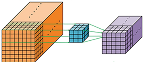
In this paper, a 3D convolutional neural network is used, the convolutional layer is the most important part of the convolutional neural network, combining the convolutional kernel with a multi-scale pixel module, as shown in Figure 2, facilitates 3D information feature extraction, the value of the neuron at the position $(\mathit{x},\mathit{y},\mathit{z})$ of the $\mathit{j}$ th feature map in the $\mathit{i}$ th convolutional layer in the 3D convolution is defined as shown in equation (1)(1) $v_{ij}^{xyz}=\mathit{f}\left(\sum _s\sum _{\mathit{m}=0}^{M_i-1}\sum _{\mathit{n}=0}^{N_i-1}\sum _{\mathit{t}=0}^{T_i-1}{w}_{ijs}^{mnt}{v}_{(i-1)s}^{(x+m)(y+n)(z+t)}+b_{\mathit{ij}}\right)$(1)

Figure 2. Three-dimensional convolution operation diagram.

(1) $v_{ij}^{xyz}=\mathit{f}\left(\sum _s\sum _{\mathit{m}=0}^{M_i-1}\sum _{\mathit{n}=0}^{N_i-1}\sum _{\mathit{t}=0}^{T_i-1}{w}_{ijs}^{mnt}{v}_{(i-1)s}^{(x+m)(y+n)(z+t)}+b_{\mathit{ij}}\right)$(1)

The formula, $\mathit{i}$ represents the number of layers of the convolutional layer, $\mathit{s}$ is the feature map from the feature map in the $(\mathit{i}-1)$ layer to the feature map of the current $\mathit{i}$ layer, $M_i$and $M_i$ represent the size of the convolution kernel in the spatial domain, $T_i$ represents the size of the convolution kernel in the spectral domain, $(\mathit{m},\mathit{n},\mathit{t})$ represents the position of the feature block in the 3D convolution, and represents the convolution between the feature block of the $w_{ijs}^{mnt}$ layer and the $(\mathit{i}-1)$ layer. The weight value of the kernel $(\mathit{m},\mathit{n},\mathit{t})$. $b_{\mathit{ij}}$ denotes the bias of the $\mathit{j}$-th feature map in the $\mathit{i}$-th layer. Figure 2 Three-dimensional convolution operation diagram.

Assuming that the size of the image is $\mathit{M}\times \mathit{M}$, the convolution kernel size is $3\times 3$, the padding is $\mathit{D}$, and the step size is $\mathit{S}$, the calculation of the output feature size $\mathit{H}$ is shown in formula (2)

(2) $\mathit{H}=\frac{\mathit{M}-3+2\mathit{D}}{S}+1$(2)

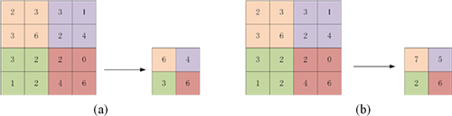
The pooling layer can be used to reduce the size of the feature space after the convolution operation, thus reducing the network parameters, speeding up the calculation, reducing the number of parameters reaching the fully connected layer, and avoiding the overfitting phenomenon. The pooling layer can be divided into two ways: Average Pooling and Max Pooling. As shown in Figure 3.

Figure 3. Pooling process. (a) average pooling; (b) max pooling.

The common activation functions Sigmoid, Tanh, ReLU, and Leaky ReLU, the ReLU activation function is used for experiments in this article.

Each node in the fully connected layer is connected to all nodes in the previous layer, and the high-dimensional feature map can be linearly stretched to convert the high-dimensional feature map into a one-dimensional vector for classification or classification in the classifier. Regression processing.

The output layer uses a Softmax classifier. In multi-classification problems, Softmax classifiers are generally used.

Channel-spatial attention mechanism module (CSAM)

The visual attention mechanism is a brain signal processor unique to human vision, whereas the attention mechanism in deep learning is based on the attentional thinking of human vision (N. Li et al., 2018). In addition, the attention model has been widely used in diverse types of deep learning tasks, such as natural language processing, image identification, and speech recognition, and is the key technology that deserves the most attention and in-depth understanding in deep learning technology. The essence of the attention mechanism is to locate the information of interest and suppress the useless information. In terms of principle, there are three main types of attention models: channel attention model, spatial attention model, and channel and spatial attention model. Inspired by the literature (Woo et al., 2018), this work introduces the CSAM module into the MMC-CNN model and focuses on characterizing the channel attention module and the spatial attention module subsequently.

The channel attention mechanism module mainly weights the channel. In a sense, channel attention focuses on the channel of interest and suppresses the weight of the uninteresting channel to a certain extent. As shown in Figure 4, first, the input feature layer is subjected to maximum pooling and average pooling operations based on width and height to obtain two feature strips, each feature strip is a one-dimensional vector, where the feature strip. The length is the number of channels of the input feature layer. The network parameters are shared through three fully connected layers of different lengths. The shared network is composed of a three-layer perceptron (MLP) and a hidden layer. At the same time, the output features are summed and mapped to [0,1], and the channel attention $M_c\in R^{\mathit{C}\times 1\times 1}$ is obtained at the same time, the greater the weight value obtained, the more important the corresponding spectral channel. Next, the number of neurons is multiplied by the number of channels of the input feature layer one by one, and finally, the input features required by the spatial attention module are output to complete the process of the channel attention mechanism. The expression of the mapping function generation process of the channel attention module is shown in formula (3):

Figure 4. Channel attention module.

(3) $\begin{array}{rl}& M_c(\mathit{F})\text{break}=\mathit{\sigma }(\mathit{MLP}(\mathit{AvgPool}(\mathit{F}))+\mathit{MLP}(\mathit{MaxPool}(\mathit{F})))\\ & =\mathit{\sigma }(W_1(W_0(F_{avg}^c))+W_1(W_0(F_{max}^c))\end{array}$(3)

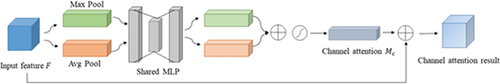
Among them, $\mathit{\sigma }$ refers to the Sigmoid activation function, $W_0\in R^{\mathit{C}/r\times C}$, $W_0\in R^{\mathit{C}/r\times C}$, $\mathit{r}$ refers to the reduction rate, $F_{avg}^c$ and refers to the average pooling feature, and the maximum pooling feature, respectively.

The spatial attention mechanism module mainly weights the spatial dimension. The goal is to focus on the more important features of the spatial shape and weaken the features of unimportant positions. It is also a supplement to the channel attention mechanism module. As shown in Figure 5, firstly, the result feature map output by the channel attention is used as the input of the spatial attention module, and a channel-based maximum pooling and flat pooling operation is performed on the input feature layer, and the number of the obtained result channels is increased, using A convolutional layer dimensionality reduction, the proportion of each feature point is obtained through the Sigmoid function, and the spatial attention feature map $M_{\mathrm{s}}$ is generated. Finally, the generated spatial attention feature map $M_{\mathrm{s}}$ is multiplied by the input feature layer to obtain the final output feature map. Spatial attention mechanism pipeline. The mapping function process expression of the spatial attention module is shown in formula (4):

Figure 5. Spatial attention module.

(4) $\begin{array}{rl}& M_s(\mathit{F})\text{break}=\mathit{\sigma }(f^{7\times 7\times 1}([\mathit{AvgPool}(\mathit{F});\mathit{MaxPool}(\mathit{F})]))\\ & =\mathit{\sigma }(f^{{\mathit{ }}^{7\times 7\times 1}}([F_{avg}^c;F_{max}^c]))\end{array}$(4)

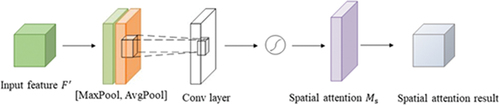
Among them, $\mathit{\sigma }$ is the Sigmoid activation function, which represents the convolution operation with the size of the convolution kernel being 7 × 7 × 1.

Introduction to the dataset

Three datasets were Selected for the experimental data: Indian Pines (IP), Pavia Center (PC), and Kennedy Space Center (KSC). The ground sample of objects was randomly dispersed and then sectioned according to a certain ratio, with 10% of each type of sample selected in the dataset. As a training set, the remaining 90% was used as a test set for the experiments.

1. Indian Pines was the first to image an Indian pine tree in Indiana, USA by the Airborne Visible Infrared Imaging Spectrometer (AVIRIS). The image size is 145 pix-els × 145 pixels, the wavelength range is 400 ~ 2500 nm, and the spatial resolution is 20 meters/pixel. Contains 220 continuously imaged ground objects, removes 20 bands that cannot be reflected by water and uses 16 types of ground objects with 1049 pixels for classification experiments. Figure 6a shows the false color image and Figure 6b shows the ground truth, and [Table 1] covers the types and the total number of samples.

   Figure 6. lndian pines dataset image. (a) false color image; (b) ground truth.

   

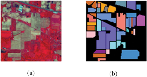
   Table 1. Indian Pines dataset coverage types and total samples.

   Class No.	Class Name	Color	Sample Number
   1	Alfalfa		46
   2	Corn-no till		1428
   3	Corn-min till		830
   4	Corn		237
   5	Grass-pasture		483
   6	Grass-trees		730
   7	Grass-pasture-mowed		28
   8	Hay-windrowed		478
   9	Oats		20
   10	Soybean-no till		972
   11	Soybean-min till		2455
   12	Soybean-clean		593
   13	Wheat		205
   14	Woods		1265
   15	Building-Grass-Trees-Drivers		386
   16	Stone-Steel-Towers		93
   Total	Class Name		10249

2. Pavia Center is a hyperspectral dataset acquired by the airborne Reflection Op-tical Spectral Imager (ROSIS) of Pavia, Italy, with an image size of 1096 pixels × 715 pixels, a spatial resolution of 1.3 m/image, and a wavelength range of 430 ~ 860 nm, using 148,152 pixels of nine contained features for classification experiments. Figure 7a shows the false color image and Figure 7b shows the ground truth, and [Table 2] covers the types and the total number of samples.

   Figure 7. Pavia center dataset image. (a) false color image; (b) ground truth.

   

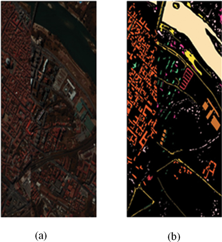
   Table 2. Pavia Center dataset coverage types and total samples.

   Class No.	Class Name	color	Sample Number
   1	Water		65971
   2	Trees		7598
   3	Asphalt		3090
   4	Self-Blocking Bricks		2685
   5	Bitumen		6584
   6	Tiles		9248
   7	Shadows		7287
   8	Meadows		42826
   9	Bare Soil		2863
   Total			148152

3. 3. The KSC and Indian Pines datasets are both taken by the AVIRIS spectrometer as well, and the data are collected at the Kennedy Space Center (KSC) in Flo-rida. The image size is 512 pixels × 614 pixels, with a spatial resolution of 18 m and a central wavelength of 400 ~ 2500 nm, and 13 species containing 5211 pixels of features were used for the classification experiments. Figure 8a shows the false color image and Figure 8b shows the ground truth, and [Table 37] covers the types and the total number of samples.

   Figure 8. KSC dataset image. (a) false color image; (b) ground truth.

   

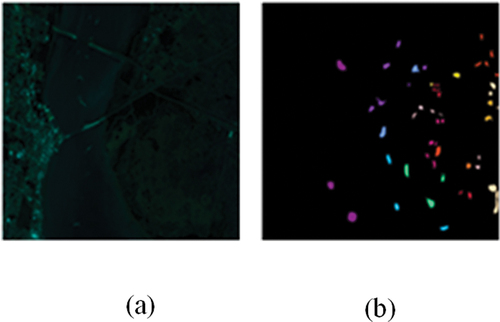
   Table 3. KSC coverage dataset types and total samples.

   Class No.	Class Name	color	Sample Number
   1	Scrub		761
   2	Willow swamp		243
   3	CP hammock		256
   4	Slash pine		252
   5	Oak/Broadleaf		161
   6	Hardwood		229
   7	Swamp		105
   8	Graminoid marsh		431
   9	Spartina marsh		520
   10	Cattail marsh		404
   11	Salt marsh		419
   12	Mudflats		503
   13	Water		927
   Total			5211

The data associated with the particular hyperspectral dataset are shown in [Table 4 near here].

Table 4. Hyperspectral dataset.

	Indian Pines	Pavia Center	KSC
Imaging spectrometer	AVIRIS	ROSIS	AVIRIS
Spectral band/nm	400 ~ 2500	430 ~ 860	400 ~ 2500
Number of bands	200	102	176
Number of cells/pixel	145 × 145	1096 × 715	512 × 614
Spatial resolution/m	20	1.3	18
Number of samples	10249	148152	5211
Feature Categories	16	9	13

Evaluation indicators

To demonstrate the classification performance of the MMC-CNN model and CSAM-MMC model method proposed in this paper, two representative methods based on the traditional SVM method and deep learning-based HSI classification, such as CNN and DCCNN, are used as comparison methods. The classification performance of each algorithm is evaluated by three commonly used indicators: overall classification accuracy (OA), average classification accuracy (AA), and kappa coefficient. These three metrics are significant indicators of the performance of the classification algorithm, and the larger the value, the more effective the classification is. Through the evaluation of these indicators, the classification performance of various algorithms can be obtained, so as to judge the validity and application prospects of MMC-CNN and CSAM-MMC models. The following is a brief description of the three indicators:

Overall classification accuracy (overall accuracy, OA)

The overall classification accuracy refers to the ratio of the number of correctly classified samples in the results to the total number of samples that need to be classified after the hyperspectral samples are classified. The calculation formula of OA is shown in formula (5):

(5) $\mathit{OA}=\frac{1}{N}\sum _{\mathit{j}=1}^{N_c}{m}_{\mathit{jj}}$(5)

Among them, $\mathit{N}$ represents the total number of test samples, and $m_{\mathit{jj}}$ represents the number of correctly classified samples of the $\mathit{j}$ th class.

Average classification accuracy (average accuracy, AA)

The average classification accuracy AA refers to the mean value of each class sample that is correctly classified in the result after the hyperspectral sample is classified, and its calculation formula is shown in formula (6):

(6) $\mathit{AA}=\frac{\sum _{\mathit{j}=1}^{N_c}\frac{{\mathit{m}}_{\mathit{jj}}}{m_{+\mathit{j}}}}{N_c}$(6)

Among them, $m_{+\mathit{j}}$ is the summation of the numbers in the $\mathit{j}$ th column, that is, the total number of samples of the $\mathit{j}$ th class.

Kappa

The Kappa coefficient is an index for evaluating the effect of hyperspectral images. The Kappa coefficient is calculated by the discrete analysis method, and the classification results are compared with the actual situation, which has a good judgment on the results of the algorithm. The Kappa coefficient is an accurate evaluation index when evaluating the hyperspectral classification effect, and the calculation formula is shown in formula (7):

(7) $\mathit{Kappa}=\frac{\mathit{N}\sum _{\mathit{j}=1}^{N_c}{m}_{\mathit{jj}}-\sum _{\mathit{j}=1}^{N_c}{m}_{\mathit{j}+}{m}_{+\mathit{j}}}{N^2-\sum _{\mathit{j}=1}^{N_c}{m}_{\mathit{j}+}{m}_{+\mathit{j}}}$(7)

Among them, $\mathit{N}$ is the number of pixels tested in the total training samples, and “$+$” means summation on rows or columns. Compared with the overall classification accuracy and the average classification accuracy, it uses the confusion matrix, so the reflected data is more comprehensive.

A multi-scale multi-channel convolutional neural network model (MMC-CNN)

Method

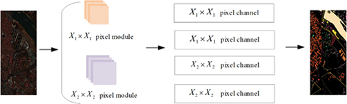
When most CNN networks extract features from hyperspectral remote sensing images since 1D-CNN can only extract spectral information and 2D-CNN can only ex-tract spatial information, important feature information of adjacent pixels will be lost, and only relatively single, shallow spectral feature information or spatial information of the layer, the feature extraction is relatively insufficient, resulting in inaccurate model classification accuracy. However, hyperspectral image classification performance is highly dependent on spatial and spectral information. So as to improve the classification accuracy of various objects and extract deeper spectral space information, it is often necessary to use 3D-CNN convolution to increase the number of layers of the neural network or build a deeper network framework. Therefore, this paper uses a parallel convolutional neural (MMC-CNN) model with four channels, as shown in Figure 9 based on the MMC-CNN network model structure diagram. It mainly consists of three stages: pixel module cropping, feature fusion extraction, and label recognition. In each channel, two-pixel modules of different scales are input to obtain channel information, and then the data cube column vectors generated by convolution are concatenated together for the final classification step.

Figure 9. This is a figure. Schemes follow the same formatting.

First of all, the HSI image is a three-dimensional cube structure, the structure form is $\mathit{H}\times \mathit{W}\times \mathit{B}$, $\mathit{H}$ represents the height of the HSI image, $\mathit{W}$ represents the width of the HSI image, and $\mathit{B}$ represents the number of HSI spectral bands. Our goal is to predict the label category for each pixel in the hyperspectral image object category. In the preprocessing stage, the hyperspectral raw data is centered on a single pixel, and divided into two different scale modules according to the size value set by the multi-scale, and the adjacent pixel modules are obtained. At the same time, the relevant feature in-formation of the hyperspectral pixel module is obtained. The pixel modules are used as input units and are input into channels of different sizes.

Second, the two kinds of pixel modules are respectively input into the multi-channel convolutional neural network, and the three-dimensional convolution kernel is used as a feature extractor in each channel, which can effectively capture the characteristics of different levels of detail of the input information, and combine spatial and spectral information. Perform deep feature extraction.

Finally, the comprehensive feature map after the parallel four-branch channel feature extraction is input to the one-dimensional fully connected layer, and then the classification result is output through the Softmax classifier.

Results

This experiment is based on the Keras framework with Tensorflow as the backend calculation. The Keras framework has the characteristics and advantages of high modularity, extremely simplified API, and easy scalability. The GPU is used for acceleration during the experiment, and the environment used in the experiment is shown in [Table 5].

Table 5. Experimental hardware and software environment.

Hardware environment	Software Environment
Processor: Inter(R) Core(TM) i9-9900K	Windows 10
GPU: NVIDIA Quadro RTX 4000	CUDA 11.0
RAM: 32GB	Python3.7.13+Tensorflow2.1.0+Keras2.3.1

This paper adopts the MMC-CNN model. To verify the performance of the pixel module in this paper and obtain a better network structure, this paper quantitatively analyzes the scale and number of the input pixel modules, as shown in [Table 6] Five methods are selected for comparative experiments. The first method adopts all 1 × 1 pixel modules; 3 × 3 pixel modules; the fourth type uses 3 × 3 pixel modules for the first two channels, and 5 × 5 pixel modules for the last two channels; the fifth type uses all 5 × 5 pixel modules.

Table 6. Multi-scale pixel module structure.

Scale size	1st channel	2nd channel	3rd channel	4th channel
1	1 × 1	1 × 1	1 × 1	1 × 1
2	1 × 1	1 × 1	3 × 3	3 × 3
3	3 × 3	3 × 3	3 × 3	3 × 3
4	3 × 3	3 × 3	5 × 5	5 × 5
5	5 × 5	5 × 5	5 × 5	5 × 5

As shown in Figure 10, 1 + 1 means that all are 1 × 1 pixel modules, 1 + 3 means that the first two channels are 1 × 1 pixel modules, the last two channels are 3 × 3 pixel modules, and so on. The average classification accuracy AA is selected as the classification index. In the experiment, as the pixel module scale increases continuously, the average classification accuracy will increase accordingly, but the complexity will also be higher, the running speed will be slower and the time will be too long. It can be seen from Figure 10 that the classification accuracy improves the most in the process from 3 + 3 to 3 + 5, and the difference in classification accuracy from 3 + 5 to 5 + 5 is only about 0.05%. Considering the running time and performance of experimental equipment, In this paper, the 3 + 5 pixel module is selected as the processing unit for subsequent experiments.

Figure 10. Average precision of multi-scale pixel modules.

In our experiments, in order to validate the effectiveness of the proposed method in this paper, we compared the proposed MMC-CNN framework with other methods, i.e. the traditional classical hyperspectral image classification methods SVM (Melgani & Bruzzone, 2004), CNN (Slavkovikj et al., 2015), DCCNN (Haokui et al., 2017a) methods and the advanced SSRN (Zhong et al., 2018), DSSIR-Net (Roy, Manna, et al., 2021) methods. All experimental models are divided into 1:9 ratio for training and test sets, $l_r=0.001$, $\mathit{epoch}=200$, $\mathit{batch}\_\mathit{size}=128$, and the experimental results are run independently for 20 times before selecting the optimal results.

The classification results of Indian Pines dataset, Pavia Center dataset, and KSC dataset are analyzed as follows: [Table 7], [Table 8], and [Table 9] show the results of the classification of each feature on the dataset, and Figures 11, 12, and 13 show the visualization of each feature after classification.

Figure 11. Classification results of different methods for Indian pines hyperspectral images. (a) false color image; (b) ground truth; (e) SVM; (d) CNN; (e) DCCNN; (f) MMC-CNN.

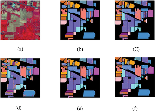
Figure 12. Classification results of different methods for pavia center hyperspectral images. (a) false color image; (b) ground truth; (c) SVM: (d) CNN; (e) DCCNN; (f) MMC-CNN.

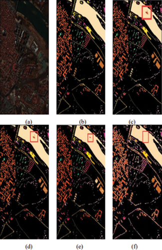
Figure 13. Classification results of different methods for KSC hyperspectral images. (a) false color image; (b) ground truth; (e) SVM; (d) CNN; (e) DCCNN; (f) MMC-CNN.

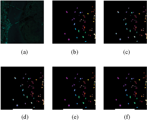
Table 7. Indian pines hyperspectral imagery dataset classification accuracy (%).

Class No.	SVM	CNN	DCCNN	SSRN	DSSIR-Net	MMC-CNN
1	57.78	97.40	97.46	97.36	97.68	97.56
2	68.70	92.56	98.12	95.49	96.53	98.26
3	72.88	87.74	91.27	95.21	96.61	92.02
4	45.94	91.39	91.56	96.21	94.78	96.45
5	82.12	96.06	96.27	97.67	98.23	97.26
6	84.15	96.41	96.43	98.56	99.21	95.47
7	87.90	94.46	95.57	92.21	93.89	95.28
8	87.15	98.95	99.58	95.35	99.86	98.52
9	72.43	92.26	90.24	89.34	82.56	93.06
10	70.44	89.92	92.46	92.24	95.36	97.51
11	68.38	93.35	93.40	97.28	96.31	95.82
12	63.61	95.24	98.39	96.87	98.03	98.81
13	88.10	94.15	97.58	99.81	100.0	97.84
14	92.06	96.34	96.75	97.54	97.95	98.89
15	64.44	92.32	93.24	95.94	95.85	96.21
16	90.15	95.92	95.69	94.18	96.34	95.84
OA	74.78	95.23	95.84	96.86	97.06	97.23
AA	74.58	95.86	96.28	96.04	96.56	97.45
Kappa	74.53	94.35	95.64	96.13	96.49	96.88

Table 8. Pavia center hyperspectral imagery dataset classification accuracy (%).

Class No.	SVM	CNN	DCCNN	SSRN	DSSIR-Net	MMC-CNN
1	93.46	99.45	99.79	99.01	99.16	99.98
2	94.28	94.18	95.20	98.99	100.0	98.45
3	62.46	96.46	96.80	96.97	98.57	98.90
4	85.05	92.73	94.45	97.56	97.98	97.20
5	97.42	97.25	95.42	98.02	97.98	99.99
6	85.48	92.34	90.10	99.31	99.23	98.69
7	64.53	92.36	92.29	99.04	99.21	99.39
8	74.77	99.16	99.64	82.82	97.86	99.79
9	98.15	95.23	95.07	97.56	98.13	97.33
OA	87.98	96.16	97.82	97.45	99.26	99.50
AA	84.24	95.86	97.25	97.06	98.89	99.38
Kappa	0.8337	0.9431	0.9690	96.48	98.26	99.02

Table 9. KSC hyperspectral imagery dataset classification accuracy (%).

Class No.	SVM	CNN	DCCNN	SSRN	DSSIR-Net	MMC-CNN
1	95.26	95.03	95.32	99.92	99.15	99.21
2	95.04	92.36	94.03	98.23	98.56	98.18
3	96.88	96.41	97.46	97.24	96.54	98.26
4	80.16	95.36	97.63	98.04	95.26	97.81
5	77.50	96.76	98.57	95.42	95.45	97.04
6	86.84	96.31	97.77	95.64	96.45	99.26
7	94.23	95.23	98.98	97.13	98.45	99.15
8	93.95	95.32	98.04	98.89	99.57	99.36
9	96.92	98.89	98.36	97.51	99.06	99.15
10	96.04	94.28	93.24	95.36	95.41	96.34
11	96.04	97.36	97.42	96.34	98.18	97.63
12	94.42	95.64	96.78	97.54	97.15	98.26
13	95.14	97.19	98.25	97.69	97.21	98.39
OA	94.69	96.26	97.25	98.46	98.84	99.18
AA	93.35	95.14	96.17	98.89	99.25	99.56
Kappa	93.09	94.62	95.99	97.87	98.54	98.87

The validity and feasibility of this paper’s algorithms are first verified in Indian Pines dataset. The classification results of a total of six algorithms for the comparison test and this paper’s model experiments are shown in Figure 11 after visualization, and the detailed classification result data of each algorithm is shown in [Table 7]. The overall classification accuracy of the traditional SVM algorithm is only 74.78%, and the text framework is 2% and 1.39% higher compared to the CNN framework and DCCNN framework, and 0.37% and 0.17% higher compared to the advanced SSRN framework and DSSIR-Net framework. Figure 11 visualizes the classification results of several algorithms. By comparing Figure 11c with Figure 11b, it can be seen that although the SVM algorithm distinguishes the 16 land classes somewhat, the image results still show many fuzzy spots and display large mislabeling on the classification map. Mainly due to the fact that the Indian Pine dataset contains fewer labeled samples, the number of fuzzy spots is reduced a lot by using convolution kernel for feature extraction in Figure 11d–h to achieve better null spectrum information. Text proposed MMC-CNN (Figure 11f) multi-channel simultaneous deep feature acquisition of features, great extent of accurate classification of all features.

Then the validity and feasibility of the algorithms in this paper are verified in the Pavia Center dataset. The classification results of a total of six algorithms for the comparison test and the experiments of this paper are shown in Figure 12 after visualization, and the detailed classification result data of each algorithm is shown in [Table 8 near here], with the best results shown in bold. The overall classification accuracy of the traditional SVM algorithm is only 87.98%, and the method of text is 3.34% and 1.68% higher compared to the CNN framework and DCCNN framework. Figure 12 visualizes the classification results of several algorithms. As the location of the features marked by the red box in Figure 12, comparing Figure 12(c–h) with Fig. (b) in turn, it is obvious to see that SVM, CNN, DCCNN, SSRN, and DSSIR-Net algorithms are not classified more or less accurately, and the text algorithm, MMC-CNN (Figure 12h), has a better classification effect, which is in line with Fig. (b), which shows the real feature labeling distribution is basically consistent, and at the same time, it shows the superiority of text algorithm MMC-CNN.

Finally the validity and feasibility of the algorithms in this paper are verified in the KSC dataset. Comparison test and this paper experiments a total of six algorithms classification results after visualization is shown in Figure 13, each algorithm’s detailed classification results data is shown in [Table 9], the best results are shown in bold. The overall classification accuracy of the traditional SVM algorithm is only 94.69%, and the method of text is 2.92% and 1.93% higher compared to the deep learning methods CNN and DCCNN. Figure 13 visualizes the classification results of several algorithms. Due to the characteristics of the KSC dataset itself, all six algorithms have better performance in edge processing, and the method in this paper performs better in the overall evaluation metrics, even though it is not the optimal result in each class of classification. Figure 13c,d have more serious misclassification phenomena in classification, and the overall effect of Figure 13e–h) classification has been improved, but in the minutiae, the classification effect of Figure 13h is more accurate.

A multi-scale multi-channel convolutional neural network model (CSAM-MMC) introducing spatial-channel attention mechanism

Method

In order to reduce parameter redundancy and improve the performance of the model, the text improves the original model MMC-CNN network structure, reduces the convolution and pooling modules, introduces the channel-spatial attention mechanism module, and designs a channel-spatial attention. The multi-scale multi-channel convolutional neural network (CSAM-MMC) model of the force mechanism module, as shown in Figure 14, combines the advantages of the convolution module and the attention mechanism module, and pays more attention to the useful spatial spectrum from the two aspects of space and channel information to effectively capture image features.

Figure 14. CSAM-MMC network structure diagram.

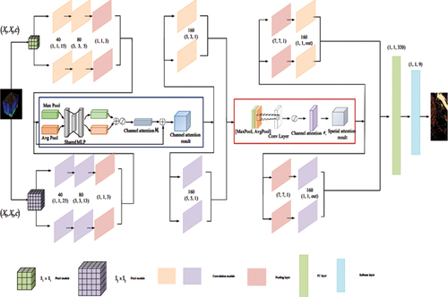
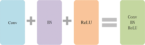
In the CSAM-MMC model, after each convolutional layer operation is completed, a BN layer is passed through, and then the ReLU activation function is used for activation. In order to facilitate the description of the experiment, this paper uses a convolutional layer, a BN layer, and a layer activation function ReLU layer is named a convolution module, as shown in Figure 15.

Figure 15. ConYolution module.

In the CSAM-MMC network structure, taking the Pavia Center data set as an example, the original hyperspectral data whose size is small and large $\mathit{H}\times \mathit{W}\times \mathit{B}$ is divided into $X_1\times X_1$ scale module and $X_2\times X_2$ scale module by the set value, and the height Spectral pixel module-related feature information. The acquired pixel modules are used as input units and are input to the channels of different sizes of the CSAM-MMC network. The input sizes are $1\times X_1\times X_1\times \mathit{B}$ and $1\times X_2\times X_2\times \mathit{B}$, and $\mathit{B}$ represents the number of bands of the hyperspectral image.

In the network structure, through two convolution modules, pooling layer, channel attention module, convolution module, spatial attention module, pooling layer, and convolution module in turn, after deep feature extraction, the comprehensive feature map is passed. The only one-dimensional fully connected layer and the Softmax classifier output the classification probabilities of various samples. In the first convolution module, the step size is 1, Padding is set to “valid”, the convolution kernel size is (1, 1, 15) and (1, 1, 25), and the spectral channel is reduced, and then The spatial information features are extracted through the convolution modules (3, 3, 5) and (3, 3, 13), and input to the maximum pooling layer to obtain the feature map. The obtained input feature map is first passed through the channel attention mechanism module, and the maximum pooling (7, 7, 1) and average pooling (7, 7, 1) operations based on width and height are used in the channel attention mechanism module to obtain Two feature strips are then applied to each feature through the shared network, and the output features are added and summed to obtain the size of (9 × 9 × 60) and (11 × 11 × 60) channel attention results. In the feature map, the channels of interest are focused on and strengthened in the process, and the channels of no interest are suppressed and reduced in weight. The resulting features of the channel attention module go through a convolution module with a size of (3, 3, 1) and (5, 5, 1), and a feature map with a shape of (7 × 7 × 60, 160) is obtained as a spatial attention mechanism module. The input feature map. In the spatial attention mechanism module, a convolution kernel with a size of (7, 7, 1) is applied to generate a spatial attention map and a spatial feature with a size of (9 × 9 × 60) is generated as a result, and finally passed through A pooling layer and a convolutional layer. After the shape of the feature map of the attention mechanism module does not change, the output feature maps of the four channels are input to the one-dimensional FC layer, and after normalization, the Softmax classifier is used to output the classification results of each object.

In hyperspectral image classification, channel direction mainly emphasizes spectral features while suppressing useless spectral features, while spatial direction mainly focuses on input scale modules. In the model, the ReLU activation function with a faster convergence speed is selected, and the output layer uses the Softmax function.

The advantage of using the Adam optimizer in the model training process is that after the bias correction, the learning rate of each iteration can be kept in the correct range, making the parameter change more stable. The learning rate is 0.001; using the cross-entropy loss function, its expression function is shown in formula (8)

(8) $\mathit{L}=\frac{1}{N}\sum _i\sum _{\mathit{c}=1}^M{y}_{\mathit{ic}}log(p_{\mathit{ic}})$(8)

Among them, $\mathit{M}$is the number of categories, $y_{\mathit{ic}}$ refers to the sign function (0 or 1), if the true category of sample $\mathit{i}$ is equal, $\mathit{c}$takes 1, otherwise $\mathit{c}$ takes 0, and $p_{\mathit{ic}}$ is the predicted probability that the observed sample $\mathit{i}$ belongs to category $\mathit{c}$.

Results

In order to verify the effectiveness of the method in this paper, the same experimental environment and parameter configuration as the MMC-CNN model in Section III are used. Since a detailed comparison has been made with the traditional classical hyperspectral image classification methods SVM, CNN, DCCNN method and the MMC-CNN model proposed in this paper in Section III, we will not describe them all here, but only discuss the MMC-CNN model compared with the CSAM-MMC model.

The classification results of Indian Pines dataset, Pavia Center dataset, and KSC dataset are analyzed as follows: [Table 10], [Table 11], and [Table 12] show the results of the classification of each feature on the dataset, and Figures 16, 17, and Figure 18 show the visualization of each feature after classification.

Figure 16. Classification results of different methods for Indian pines hyperspectral imagery: for peer review only (a) false color image: (b) ground truth: (e) MMC-CNN: (d) CSAM-MMC.

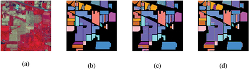
Figure 17. Classification results of different methods for pavia center hyperspectral image1y. (a) false color image: (b) ground truth: (e) MMC-CNN: (d) CSAM-MMC.

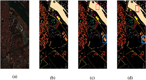
Figure 18. Classification results of different methods for KSC hyperspectral imagery. (a) false color images; (b) ground truth: (e) MMC-CNN: (d) CSAM-MMC.

Table 10. Indian pines hyperspectral imagery dataset classification accuracy (%).

Class No.	SVM	CNN	DCCNN	SSRN	DSSIR-Net	MMC-CNN	CSAM-MMC
1	57.78	97.40	97.46	97.36	97.68	97.56	97.59
2	68.70	92.56	98.12	95.49	96.53	98.26	100.00
3	72.88	87.74	91.27	95.21	96.61	92.02	96.90
4	45.94	91.39	91.56	96.21	94.78	96.45	96.35
5	82.12	96.06	96.27	97.67	98.23	97.26	98.52
6	84.15	96.41	96.43	98.56	99.21	95.47	99.75
7	87.90	94.46	95.57	92.21	93.89	95.28	95.12
8	87.15	98.95	99.58	95.35	99.86	98.52	100.00
9	72.43	92.26	90.24	89.34	82.56	93.06	94.72
10	70.44	89.92	92.46	92.24	95.36	97.51	96.82
11	68.38	93.35	93.40	97.28	96.31	95.82	97.40
12	63.61	95.24	98.39	96.87	98.03	98.81	98.39
13	88.10	94.15	97.58	99.81	100.0	97.84	98.14
14	92.06	96.34	96.75	97.54	97.95	98.89	99.84
15	64.44	92.32	93.24	95.94	95.85	96.21	95.99
16	90.15	95.92	95.69	94.18	96.34	95.84	96.08
OA	74.78	95.23	95.84	96.86	97.06	97.23	97.49
AA	74.58	95.86	96.28	96.04	96.56	97.45	97.87
Kappa	74.53	94.35	95.64	96.13	96.49	96.88	97.22

Table 11. Pavia center hyperspectral imagery dataset classification accuracy (%).

Class No.	SVM	CNN	DCCNN	SSRN	DSSIR-Net	MMC-CNN	CSAM-MMC
1	93.46	99.45	99.79	99.01	99.16	99.98	100.00
2	94.28	94.18	95.20	98.99	100.0	98.45	98.81
3	62.46	96.46	96.80	96.97	98.57	98.90	98.75
4	85.05	92.73	94.45	97.56	97.98	97.20	98.78
5	97.42	97.25	95.42	98.02	97.98	99.99	99.99
6	85.48	92.34	90.10	99.31	99.23	98.69	98.04
7	64.53	92.36	92.29	99.04	99.21	99.39	99.54
8	74.77	99.16	99.64	82.82	97.86	99.79	99.89
9	98.15	95.23	95.07	97.56	98.13	97.33	99.37
OA	87.98	96.16	97.82	97.45	99.26	99.50	99.85
AA	84.24	95.86	97.25	97.06	98.89	99.38	99.64
Kappa	0.8337	0.9431	0.9690	96.48	98.26	99.02	99.37

Table 12. KSC hyperspectral imagery dataset classification accuracy (%).

Class No.	SVM	CNN	DCCNN	MMC-CNN	CSAM-MMC
1	95.26	95.03	95.32	97.21	98.29
2	95.04	92.36	94.03	95.18	94.37
3	96.88	96.41	97.46	98.26	99.60
4	80.16	95.36	97.63	97.81	99.89
5	77.50	96.76	98.57	97.04	97.59
6	86.84	96.31	97.77	98.26	99.74
7	94.23	95.23	98.98	98.15	99.09
8	93.95	95.32	98.04	98.36	98.26
9	96.92	98.89	98.36	99.15	100.00
10	96.04	94.28	93.24	96.34	95.65
11	96.04	97.36	97.42	97.63	98.23
12	94.42	95.64	96.78	97.26	100.00
13	95.14	97.19	98.25	97.39	98.55
OA	94.69	96.26	97.25	97.85	98.56
AA	93.35	95.14	96.17	96.38	97.64
Kappa	93.09	94.62	95.99	96.57	96.52

The validity and feasibility of the CSAM-MMC model in this paper are first verified in Indian Pines dataset. Comparing the classification results of MMC-CNN model and CSAM-MMC model after visualization, as shown in Figure 16, the classification effect is more obvious in Figure 16d by comparing Figures 16c,d with Figure 16b feature labels, respectively. The MMC-CNN (Figure 16c) proposed in the text uses multi-channel convolution for deep feature acquisition of features, which greatly classifies all features accurately. The CSAM-MMC (Figure 16d) proposed in this paper pays more attention to spatial and spectral information on the basis of multi-channel network, which has a good classification effect compared with MMC-CNN (Figure 16c). The detailed classification result data for each type of feature is shown in [Table 10]. The CSAM-MMC algorithm in this paper is 0.62% higher compared to MMC-CNN.

Then the validity and feasibility of the CSAM-MMC model in this paper is verified in the Pavia Center dataset. Comparing the classification results of MMC-CNN model and CSAM-MMC model after visualization, as shown in Figure 17, the distribution is basically the same by comparing Figures 17(c) and 17(d) with the real feature labels in Figure 17b, respectively, but it can be seen from the locations of the features marked by the blue boxes in Figure 17 that there are still some spots in Figure 17c, so the CSAM-MMC algorithm is superior to the MMC-CNN algorithm. The detailed classification result data for each type of feature is shown in [Table 11 near here], and the best results are shown in bold. The CSAM-MMC algorithm in this paper is 0.35% higher compared to MMC-CNN.

Finally, the validity and feasibility of the CSAM-MMC model in this paper are verified in the KSC dataset. Comparing the classification results of MMC-CNN model and CSAM-MMC model after visualization, as shown in Figure 18, the distribution is basically the same by comparing Figures 18c,d with Figure 18b real feature labels, respectively, but in the minutiae, the classification effect of Figure 18d is slightly better, which is attributed to the fact that the CSAM-MMC method combines the deep combination of the attentional mechanism with the hyperspectral spectral features to achieve more accurate classification. The detailed classification result data for each type of feature is shown in [Table 12g], and the best results are shown in bold. The CSAM-MMC algorithm in this paper is 0.71% higher compared to MMC-CNN.

Conclusion

The performance of hyperspectral image classification in existing classification algorithms is highly dependent on spatial and spectral information, and at the same time, relevant detailed features are ignored during feature extraction of a single convolution channel, resulting in poor generalization performance of feature extraction models. This paper proposes a multi-scale multi-channel convolutional neural network (MMC-CNN) model, which extracts spectral spatial features from a deeper level, analyses the impact of using different scale pixel modules on the classification performance, and verifies the use of 3 × 3 and 5 × 5 The pixel module has the best performance for hyperspectral image classification. In order to more focus on spatial spectral feature information, a channel-spatial attention mechanism module is added to the MMC-CNN network. In this paper, we propose a multi-scale multi-channel convolutional neural network (CSAM-MMC) model that introduces a channel-spatial attention mechanism module to fully extract latent information in hyperspectral images while reducing the redundancy of convolutional pooling parameters. The experimental data can show that the network model proposed in this paper has good classification performance in the three data sets. Due to the large number of channels and the relatively large amount of parameter calculation, the running speed of the model in this paper is relatively slow. In the follow-up research, the calculation speed can be further improved while ensuring classification accuracy.

Acknowledgments

Thanks are due to Mr. Chaozhu Zhang for his valuable comments on writing the paper and Dan Xue for his assistance in the experimental process.

Disclosure statement

No potential conflict of interest was reported by the author(s).

Additional information

Funding

This research received no external funding.

References

- Asker, M. E. (2023). Hyperspectral image classification method based on squeeze-and-excitation networks, depthwise separable convolution and multibranch feature fusion. Earth Science Informatics, 16(2), 1427–20. https://doi.org/10.1007/s12145-023-00982-0
- Awad, M. (2014). Sea water chlorophyll-a estimation using hyperspectral images and supervised artificial neural network. Ecological Informatics, 24, 60–68. https://doi.org/10.1016/j.ecoinf.2014.07.004
- Camps-Valls, G., Gomez-Chova, L., Munoz-Mari, J., Vila-Frances, J., & Calpe-Maravilla, J. (2006). Composite kernels for hyperspectral image classification. IEEE Geoscience & Remote Sensing Letters, 3(1), 93–97. https://doi.org/10.1109/LGRS.2005.857031
- Chen, Y., Lin, Z., Zhao, X., Wang, G., & Gu, Y. (2014). Deep learning-based classification of hyperspectral data. IEEE Journal of Selected Topics in Applied Earth Observations & Remote Sensing, 7(6), 2094–2107. https://doi.org/10.1109/JSTARS.2014.2329330
- Dong, S., Feng, W., Quan, Y., Dauphin, G., Gao, L., & Xing, M. (2022). Deep ensemble CNN method based on sample expansion for hyperspectral image classification. IEEE Transactions on Geoscience & Remote Sensing, 60, 1–15. Art no. 5531815. https://doi.org/10.1109/TGRS.2022.3183189
- Du, Q. D., Zhang, L. Z., Zhang, B. Z., Tong, X., Du, P., & Chanussot, J. (2013). Foreword to the special issue on hyperspectral remote sensing: Theory, methods, and applications. IEEE Journal of Selected Topics in Applied Earth Observations & Remote Sensing, 6(2), 459–465. https://doi.org/10.1109/JSTARS.2013.2257422
- Fakhrullin, R., Nigamatzyanova, L., & Fakhrullina, G. (2021). Dark-field/hyperspectral microscopy for detecting nanoscale particles in environmental nanotoxicology research. Science of the Total Environment, 772, 145478. https://doi.org/10.1016/j.scitotenv.2021.145478
- Fang, B., Han, G., Zheng, X., & He, J. (2021). Hyperspectral image classification using multi-channel lightweight CNN ensemble framework based on band clustering. ICMLCA 2021; 2nd International Conference on Machine Learning and Computer Application (pp. 1–6). Shenyang, China.
- Feng, J., Wu, X., Shang, R., Sui, C., Li, J., Jiao, L., & Zhang, X. (2021, June). Attention multibranch convolutional neural network for hyperspectral image classification based on adaptive region search. IEEE Transactions on Geoscience and Remote Sensing, 59(6), 5054–5070. https://doi.org/10.1109/TGRS.2020.3011943
- Firat, H., Asker, M. E., Bayindir, M. İ., & Hanbay, D. (2023). 3D residual spatial–spectral convolution network for hyperspectral remote sensing image classification. Neural Computing & Applications, 35(6), 4479–4497. https://doi.org/10.1007/s00521-022-07933-8
- Gevaert, C. M., Suomalainen, J., Tang, J., & Kooistra, L. (2015, June). Generation of spectral–temporal response surfaces by combining multispectral satellite and hyperspectral UAV imagery for precision agriculture applications. IEEE Journal of Selected Topics in Applied Earth Observations & Remote Sensing, 8(6), 3140–3146. https://doi.org/10.1109/JSTARS.2015.2406339
- Ghaderizadeh, S., Abbasi-Moghadam, D., Sharifi, A., Zhao, N., & Tariq, A. (2021). Hyperspectral image classification using a hybrid 3D-2D convolutional neural networks. IEEE Journal of Selected Topics in Applied Earth Observations and Remote Sensing, 14, 7570–7588. https://doi.org/10.1109/JSTARS.2021.3099118
- Hang, R., Li, Z., Liu, Q., Ghamisi, P., & Bhattacharyya, S. S. (2021, March). Hyperspectral image classification with attention-aided CNNs. IEEE Transactions on Geoscience and Remote Sensing, 59(3), 2281–2293. https://doi.org/10.1109/TGRS.2020.3007921
- Jiang, J., Ma, J., Chen, C., Wang, Z., Cai, Z., & Wang, L. (2018, August). SuperPCA: A superpixelwise PCA approach for unsupervised feature extraction of hyperspectral imagery. IEEE Transactions on Geoscience & Remote Sensing, 56(8), 4581–4593. https://doi.org/10.1109/TGRS.2018.2828029
- Li, W., Chen, C., Su, H., & Du, Q. (2015, July). Local binary patterns and extreme learning machine for hyperspectral imagery classification. IEEE Transactions on Geoscience and Remote Sensing, 53(7), 3681–3693. https://doi.org/10.1109/TGRS.2014.2381602
- Li, T., Zhang, X., Zhang, S., & Wang, L. (2022). Self-supervised learning with a dual-branch ResNet for hyperspectral image classification. IEEE Geoscience & Remote Sensing Letters, 19, 1–5. Art no. 5512905. https://doi.org/10.1109/LGRS.2021.3107321
- Li, N., Zhao, X., Ma, B., & Zou, X. (2018). A visual attention model based on human visual cognition[C/OL]//advances in brain inspired cognitive systems. Springer.
- Li, R., Zheng, Zheng, S., Duan, C., Yang, Y., & Wang, X. (2020). Classification of hyperspectral image based on double-branch dual-attention mechanism network. Remote Sensing, 12(3), 582. https://doi.org/10.3390/rs12030582
- Lu, P., Jiang, X., Zhang, Y., Liu, X., Cai, Z., Jiang, J., & Plaza, A. (2023). Spectral–spatial and superpixelwise unsupervised linear discriminant analysis for feature extraction and classification of hyperspectral images. IEEE Transactions on Geoscience & Remote Sensing, 61, 1–15. Art no. 5530515. https://doi.org/10.1109/TGRS.2023.3330474
- Melgani, F., & Bruzzone, L. (2004). Classification of hyperspectral remote sensing images with support vector machines[J/OL]. IEEE Transactions on Geoscience & Remote Sensing, 42(8), 1778–1790. https://doi.org/10.1109/TGRS.2004.831865
- Pei, S., Song, H., & Lu, Y. (2022). Small sample hyperspectral image classification method based on dual-channel spectral enhancement network[J/OL]. Electronics, 11(16), 2540. https://doi.org/10.3390/electronics11162540
- Pi, W., Du, J., Bi, Y., Gao, X., & Zhu, X. (2021). 3D-CNN based UAV hyperspectral imagery for grassland degradation indicator ground object classification research - ScienceDirect. Ecological Informatics, 62, 62. https://doi.org/10.1016/j.ecoinf.2021.101278
- Qing, Y., & Liu, W. (2021). Hyperspectral image classification based on multi-scale residual network with attention mechanism. Remote Sensing, 13(3), 335. https://doi.org/10.3390/rs13030335
- Roy, S. K., Manna, S., Song, T., & Bruzzone, L. (2021, September). Attention-based adaptive spectral–spatial kernel ResNet for hyperspectral image classification. IEEE Transactions on Geoscience and Remote Sensing, 59(9), 7831–7843. https://doi.org/10.1109/TGRS.2020.3043267
- Roy, S. K., Mondal, R., Paoletti, M. E., Haut, J. M., & Plaza, A. (2021). Morphological convolutional neural networks for hyperspectral image classification. IEEE Journal of Selected Topics in Applied Earth Observations & Remote Sensing, 14, 8689–8702. https://doi.org/10.1109/JSTARS.2021.3088228
- Shi, C., Liao, D., Zhang, T., & Wang, L. (2022). Hyperspectral image classification based on 3D coordination attention mechanism network. Remote Sensing, 14(3), 608. https://doi.org/10.3390/rs14030608
- Slavkovikj, V., Verstockt, S., Neve, W. D., Hoecke, S. V., & Walle, R. V. (2015, October 26–30). Hyperspectral image classification with convolutional neural networks. ACM International Conference on Multimedia (ACMMM), Brisbane.
- Villa, A., Benediktsson, J. A., Chanussot, J., & Jutten, C. (2011). Hyperspectral image classification with independent component discriminant analysis. IEEE Transactions on Geoscience & Remote Sensing, 49(12), 4865–4876. https://doi.org/10.1109/TGRS.2011.2153861
- Voulodimos, A., Doulamis, N., & Doulamis, A. (2018). Deep learning for computer vision: A brief review. Computational intelligence and neuroscience.
- Wang, Z., & He, B. (2011). Locality perserving projections algorithm for hyperspectral image dimensionality reduction. 19th International Conference on Geoinformatics (pp. 1–4). Shanghai, China. https://doi.org/10.1109/GeoInformatics.2011.5980790
- Woo, S., Park, J., Lee, J. Y. (2018). CBAM: Convolutional block attention module[j]. Springer.
- Xie, J., Hua, J., Chen, S., Wu, P., Gao, P., Sun, D., Lyu, Z., Lyu, S., Xue, X., & Lu, J. (2023). HyperSFormer: A transformer-based end-to-end hyperspectral image classification method for crop classification. Remote Sensing, 15(14), 3491. https://doi.org/10.3390/rs15143491
- Xu, Y., Zhang, L., & Du, B. (2018). Spectral–spatial unified networks for hyperspectral image classification. IEEE Transactions on Geoscience and Remote Sensing (pp. 1–17).
- Xu, M., Zhao, Y., Liang, Y., & Ma, X. (2022). Hyperspectral image classification based on class-incremental learning with knowledge distillation. Remote Sensing, 14(11), 2556. https://doi.org/10.3390/rs14112556
- Yang, X., Ye, Y., Li, X., Lau, R. Y. K., Zhang, X., & Huang, X. (2018, September). Hyperspectral image classification with deep learning models. IEEE Transactions on Geoscience and Remote Sensing, 56(9), 5408–5423. https://doi.org/10.1109/TGRS.2018.2815613
- Young, T., Hazarika, D., Poria, S., & Cambria, E. (2018). Recent trends in deep learning based natural language processing [review article]. IEEE Computational Intelligence Magazine, 13(3), 55–75. https://doi.org/10.1109/MCI.2018.2840738
- Zahisham, Z., Lim, K. M., Koo, V. C., Chan, Y. K., & Lee, C. P. (2023). 2SRS: Two-stream residual separable convolution neural network for hyperspectral image classification. IEEE Geoscience & Remote Sensing Letters, 20, 1–5. Art no. 5501505. https://doi.org/10.1109/LGRS.2023.3241720
- Zhai, H., Zhao, J., & Zhang, H. (2022). Double attention based multilevel one-dimensional convolution neural network for hyperspectral image classification. IEEE Journal of Selected Topics in Applied Earth Observations & Remote Sensing, 15, 3771–3787. https://doi.org/10.1109/JSTARS.2022.3162423
- Zhang, H., Li, Y., Zhang, Y., & Shen, Q. (2017a). Spectral-spatial classification of hyperspectral imagery using a dual-channel convolutional neural network. Remote Sensing Letters, 8(5), 438–447. https://doi.org/10.1080/2150704X.2017.1280200
- Zhang, H., Li, Y., Zhang, Y., & Shen, Q. (2017b). Spectral-spatial classification of hyperspectral imagery using a dual-channel convolutional neural network. Remote Sensing Letters, 8(5), 438–447. https://doi.org/10.1080/2150704X.2017.1280200
- Zheng, Y., Liu, S., Chen, H., Bruzzone, L., Ye, F., Qin, C., Wei, Z., Plaza, J., Li, J., & Plaza, A. (2024). Hybrid FusionNet: A hybrid feature fusion framework for multisource high-resolution remote sensing image classification. IEEE Transactions on Geoscience & Remote Sensing, 62, 1–14. Art no. 5401714. https://doi.org/10.1109/TGRS.2024.3385316
- Zhong, Z., Li, J., Luo, Z., & Chapman, M. (2018, February). Spectral–spatial residual network for hyperspectral image classification: A 3-D deep learning framework. IEEE Transactions on Geoscience and Remote Sensing, 56(2), 847–858. https://doi.org/10.1109/TGRS.2017.2755542