
 ?Mathematical formulae have been encoded as MathML and are displayed in this HTML version using MathJax in order to improve their display. Uncheck the box to turn MathJax off. This feature requires Javascript. Click on a formula to zoom.
ABSTRACT
This paper studied an emerging technology called Dynamic Coupling that to allow physical coupling and decoupling of railway trains at cruising speeds. A train controller and a train model were introduced and simulated using Parallel Computing. Two transitional gap references were designed (hyperbolic tangent and exponential). Two six-vehicle passenger trains coupling and decoupling on a revised real-world track section at 80 km/h were simulated. Results indicated that a certain negative (e.g. -5 mm) Reference Gap at Coupling Instant (RG@CI) and a positive (e.g. 2 mm) Reference Gap at Decoupling Instant (RG@DI) were recommended to ensure a quick coupling process and to avoid decoupling impacts. Comparatively, the exponential case was better to reduce infrastructure upgrade requirements and to achieve better comfort. The simulated train movements well matched the designed gap references; Dynamic Coupling was possible in terms of train dynamics in the simulated cases.
1. Introduction
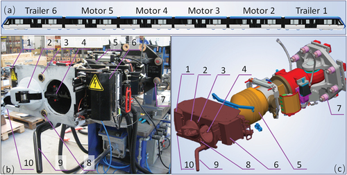
A railway train usually consists of several vehicles that can be powered (locomotives or motorized vehicles) or unpowered (wagons or trailer vehicles). Individual vehicles are commonly connected via coupling systems or coupler systems. shows a typical coupler system for passenger Electric Multiple Unit (EMU) trains. Such coupler systems are also called Digital Automatic Coupling (DAC) which can connect two consists without human interference. In this paper, a consist is defined as a vehicle unit which can be either a single vehicle, a number of vehicles or a whole train. The DAC system connects two consists mechanically, electronically, and pneumatically as shown in . Coupling guidance mechanisms help two coupler systems to align with each other vertically and laterally as well as to increase the conformality of the coupling interfaces. Currently, coupling processes by using DAC are conducted with one consist being parked stationary on track. The other consist runs into the parked consist at a low speed (e.g. maximum 5 km/h); the impact force generated during the process can then couple two consists together. Sensors are installed in the couplers that can notify drivers of the success or otherwise of the coupling process. DAC can also uncouple two consists automatically without human interference by using pneumatic cylinders that are installed in the coupler heads. Current uncoupling processes are also conducted when both consists are parked on track.
Figure 1. Vehicle coupler system: (a) EMU train, (b) actual coupler system and (c) computer graphic of coupler system. (1&6: electrical and electronic connection; 2&4: mechanical connection (cone and opening act as coupling guidance); 3&8: pneumatic connection; 5: draft gear; 7: mount to chassis; 9: coupling guidance (vertical); 10: coupling guidance (yaw)).
This paper studies an emerging technology called ‘Dynamic Coupling’ [Citation1] that aims to allow train coupling and uncoupling at cruising speeds (e.g. 80 km/h) during normal train operation. The concept of Dynamic Coupling is introduced together with the following train coupling concepts:
Manual Coupling: at least one consist remains parked during the process and an additional railway person is required to finish the coupling. An example of Manual Coupling is the European style of Hook-buffer coupler system [Citation2].
Automatic Coupling: at least one consist remains parked and railway personal is not required to finish the coupling process. An example of Automatic Coupling is the Association of American Railroads (AAR) standard automatic couplers [Citation2].
Virtual Coupling [Citation3]: two trains are virtually connected via a wireless network without physical connections and operate coordinated as one consist. Headway between two running trains should be less than the absolute brake stopping distance. Coupling and decoupling of the virtually connected trains are conducted via Train-to-Train (T2T) and/or Train-to-Infrastructure (T2I) communications.
Dynamic Coupling [Citation1]: two trains are physically coupled or decoupled when both are running at a certain speed, ideally at cruising speed (e.g. 80 km/h). The coupling and decoupling process must be controlled by computers via wireless communications.
Compared with traditional fixed block signalling systems, moving block as shown in removes fixed blocks and wayside signalling by using wireless communication between trains and control centres. Trains can operate with much shorter headways that just need to be slightly longer than the absolute brake distance of the following train. Driven by the ever-increasing traffic demand, the concept of Virtual Coupling [Citation3] as shown in is proposed to further increase railway line capacity by reducing the headway from absolute brake distances to relative brake distances. So far, Virtual Coupling has received extensive studies [Citation3–8]. However, there are still many challenges to solve before its practical implementations [Citation8].
Figure 2. Different concepts of train operation: (a) moving block, (b) virtual coupling, (c) dynamic coupling, and (d) operation for physically connected trains.
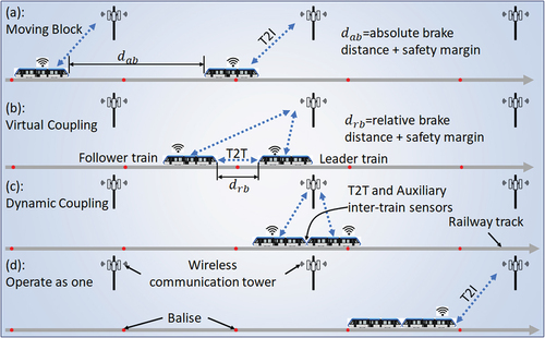
Knowing that a wireless communication infrastructure is required to achieve Virtual Coupling [Citation3], some train operational scenarios are more suitable for Dynamic Coupling rather than Virtual Coupling. One example is given in , where a connected train that departed from City A has passengers going to City B and City C. The train is then decoupled to become two trains at a cruising speed before the junction that diverges to these two destinations. Two decoupled trains will travel to City B and City C, respectively, without any stop. When travelling from City B and City C to City A, two trains can couple at cruising speed (as shown in after the junction and then travel as a connected train (as shown in ) to City A. In the Dynamic Coupling case, investment for extra wireless communication infrastructure can be significantly less as shown in .
Figure 3. A scenario that suits dynamic coupling [Citation1].
![Figure 3. A scenario that suits dynamic coupling [Citation1].](/cms/asset/b521f7a7-dd13-4116-8c74-35aa670cf67b/tjrt_a_2169963_f0003_oc.jpg)
Dynamic Coupling is an emerging technology that has not yet been systematically studied. Thanks to the recent developments in road vehicle platooning [Citation9–12] and railway Virtual Coupling [Citation3–8], the required research and development of wireless communication and system control for Dynamic Coupling can significantly benefit from the corresponding aspects addressed in platooning and Virtual Coupling. Coupling system designs can also benefit from existing research and development of DAC. However, it must be pointed out that previously designed DAC and system control technologies cannot be directly used for Dynamic Coupling. Many challenges are still to be identified and solved before the practical applications of this emerging technology.
This paper focuses on the simulations of train control and system dynamics of the Dynamic Coupling technology. Section 2 introduces a train controller that can be used to achieve Dynamic Coupling. Section 3 introduces the design of transitional gap references for the coupling and decoupling processes. Section 4 introduces the modelling of train dynamics and simulation method. Section 5 presents case studies to demonstrate the simulation of train control and dynamics d. Section 6 concludes this paper.
2. Adaptive dynamic coupling controller design
Previous studies [Citation7,Citation9] have introduced an adaptive platoon controller that can be used for Dynamic Coupling. The controller used a second-order train motion model that considered various forces including resistance forces, traction/brake (T/B) and track gradient forces:
where stands for the mass of the follower train,
is the train acceleration,
and
denote the actual traction/brake (T/B) force and the generally unknown nonlinear resistance forces on the follower train, respectively,
represents the actuation delay, and
denotes the computed control input. Specifically, the first equation above is related to the force equilibrium for the train longitudinal motions, while the second equation above details how the computed input is transformed into the actual T/B force. The primary objective of the controller was to enable the follower train to track and follow the leader train from an arbitrary initial condition (location, speed and acceleration), and eventually achieve the same speed (and acceleration) as the leader train while observing a dynamic gap reference
as required. Compared with the Virtual Coupling application [Citation7], the final gap reference in Dynamic Coupling is zero. And after the successful physical coupling of two trains, the controller needs to be disengaged and the follower train operates by directly following the commands from the leader train. More details about the controllers can be found in References [Citation7,Citation9].
3. Transitional gap reference design
The previous descriptions about the Dynamic Coupling controller indicate that a gap reference is needed to guide two adjacent trains to approach or separate from each other. This section designs the gap reference for the Dynamic Coupling controller. The decoupling process can be regarded as the reverse of the coupling process; therefore, the design is mainly focused on the coupling process. The first question to answer is when should the Dynamic Coupling process start? Or how far away should the follower train start approaching from? In this study, the starting gap reference was designed as shown in and by adapting the approach specified in the IEEE 1474.1 standard. The designed starting gap reference makes sure that, before the Dynamic Coupling, two trains run safely with a relative brake distance under the Virtual Coupling mode. And the starting reference assumes that the leader train sends emergency brake information to the follower train with a signal delay and that the follower train was having a maximum traction acceleration. In addition, speed sensor errors and localization sensor errors were assumed to overestimate the leader train’s position/speed and underestimate the follower train’s position/speed. After summing all distances, a safety factor of 1.3 was applied as an engineering norm. The gap reference design can be mathematically expressed as:
Figure 4. Starting gap reference design for dynamic coupling.
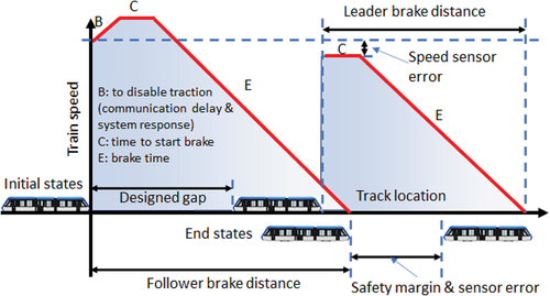
where and
are the displacement differences in Section B and Section E, respectively, shown in ,
is the designed gap reference, and the meanings of the rest of the notations can be found in . In this paper, the simulation cases considered two passenger trains with a cruising speed of 80 km/h. By using the parameters listed in , the starting gap reference was designed as 34 m (rounded up from 33.13 m). The 80 km/h simulation was selected as an acceptable cruising speed for passenger trains. High or low cruising speeds can also be studied by adjusting the model (EquationEquation (4)
(4)
(4) and subsequent gap references); the method presented in this paper is not limited specific cruising speeds.
Table 1. Parameters used for starting gap reference design.
Having designed the starting gap reference, two functions were investigated to generate the transitional profiles. The first one is based on the hyperbolic tangent function:
where is the transitional gap reference,
is a parameter to control the approaching and separation speed,
is the middle time point of the coupling process (when relative speed reaches maximum), and ‘
’ was set to be ‘-’ for the coupling process or ‘+’ for the decoupling process. While designing the transitional gap reference, three constraints were considered: (1) the maximum relative speed should not be greater than 5 km/h which is often the maximum impact speed during the normal Automatic Coupling process as discussed in Section 1; (2) the maximum acceleration should not be greater than 1.5 m/s2 with consideration of passenger comfort [Citation13]; and (3) the maximum jerk should not be greater than 0.9 m/s3 also with consideration of passenger comfort. shows the relative motions between the leader and follower trains with
(cruising speed = 80 km/h and initial gap = 34 m). In this case, the maximum relative speed, acceleration, and jerk were 1.39 m/s (5.0 km/h), 0.09 m/s2, and 0.02 m/s3, respectively, as shown in . The main constraint for the transitional gap reference design is the relative speed. When the relative speed reaches its limit, the corresponding acceleration and jerk are still well below their limits.
Figure 5. Gap references: (a) hyperbolic tangent function for distance and (b) exponential function for acceleration.
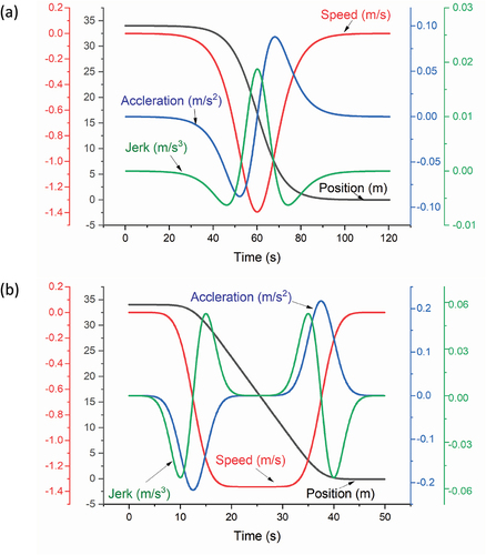
Table 2. Maximum values of the gap references.
Observing the transitional gap reference generated by using the hyperbolic tangent function, , it can be seen that there is a continuous change of acceleration from negative to positive. This may require the T/B forces to change from negative to positive without meaningful transitions via zero T/B force states, i.e. idling states. From a train dynamic perspective, transition states, for example, staying at an idling state for 5 s between switches from traction to brake or from brake to traction, are required to minimize longitudinal impacts. Having understood this, a second transitional gap reference function based on exponential functions was designed:
where is the acceleration of the follower;
is the designed maximum acceleration;
is time;
is the middle point of the coupling process; and
is controlling parameter to adjust the shape of the acceleration profile. Different from the hyperbolic tangent function case, the exponential function case starts from the acceleration. Relative velocities, distance gaps and jerks can be derived from the acceleration. shows the relative motions with the parameters of
and
; corresponding maximum values are listed in . Similar to the hyperbolic tangent function case, the maximum values of the exponential function case were also limited by the maximum relative speed, i.e. 5 km/h. Corresponding maximum acceleration and jerk were again well below limits.
EquationEquation (6)(6)
(6) can be regarded as the combination of two mirrored normal distribution profiles. Compared to the hyperbolic tangent function case, the exponential function case placed a transition between negative accelerations and positive accelerations. And the length of the transition was mainly controlled by EquationEquation (7)
(7)
(7) . It can be interpreted that beyond the
of the normal distribution (99% possibility), there was at least five more seconds in each half of the acceleration profile. This allowed roughly 10 s of transition period.
4. Train dynamics and simulation
The studied trains in the paper were passenger trains that each consists of six vehicles including four motors and two trailers as shown in . The vehicle dynamics model is shown in . It is a two-dimensional (2D) model that focuses on body motions in the longitudinal-vertical plane. Each vehicle model has seven rigid bodies; and each body has three Degrees-of-Freedom (surge, bounce, and pitch). Force elements considered in the vehicle model include wheel-rail contact forces, primary suspension forces, secondary suspension forces, rolling resistance, curving resistance, track gradient forces and T/B forces. Wheel-rail contact forces were modelled by using the Hertz theory, Hertzian stiffness and Polach model [Citation14]. By using the 2D simplification, it was assumed that all wheelsets stay at the centre of the track and the lateral radius of the wheels can therefore be regarded as constant during the simulations. By using a nonlinear Hertzian stiffness and basic multibody dynamics simulations, normal forces of the wheel-rail contact can be determined. This normal force can then be used to determine contact geometries as the wheel lateral radius is assumed as constant. Having determined the normal contact forces and contact geometry, tangential forces can then be determined by using basic creepage calculations and the Polach model. It is also noted that, during the normal force calculations, the Federal Railroad Administration (FRA) Class 6 track irregularity (vertical only) was used. Primary and secondary suspension [Citation15] forces were simply modelled as spring-damping combinations. Model parameters and validations can be found in [Citation7].
Figure 6. 2D train dynamics model: (a) vehicle model, (b) draft gear characteristics, and (c) traction and dynamic brake characteristics.
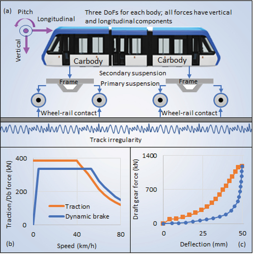
Rolling resistance and curving resistance were modelled by using an empirical formula as widely used in train dynamics simulations [Citation16]. T/B forces of the leader train were generated by using a Proportional – Integral–Derivative (PID) controller by following a constant speed limit. For the follower train, T/B forces were generated by using the Dynamic Coupling controller as presented in Section 2. Both traction and Dynamic Brake (DB) forces have used force limits as shown in . Having developed individual vehicle models, these models were then connected by draft gear force models to form trains. The draft gear model was developed by using the look-up table method and had characteristics as shown in with zero coupler slack.
Having developed the train dynamics model, PID-based Automatic Train Operation (ATO) controller, and Dynamic Coupling controller, a parallel computing scheme as used in [Citation7] was used to conduct the simulations. The simulation method used the Message Passing Interface (MPI) [Citation17,Citation18] to facilitate the parallel computing function. Specifically, the MPI algorithm starts computer cores for the total
vehicles that are simulated in the model. Among these computer cores, Core 0 is used as the master core to coordinate the simulation process and controller simulations. Cores
are then used to conduct dynamics simulations for vehicles
in the parallel computing fashion. More details of the parallel simulation method can be found in [Citation7].
The coupling process can be simulated by setting the coupler force between the leader train and the follower train constantly to zero before the relative position of these two trains are greater than zero. Once the relative position reaches a negative value (two trains are in contact), the coupler force model is then set as a normal coupler force model. The decoupling process can be simulated similarly by setting the coupler force between the leader train and the follower train constantly to zero (if the relative position is positive) after the decoupling command was issued.
5. Case studies
Case studies were conducted using the train model and simulation method developed in Section 4 to simulate the Dynamic Coupling process on a revised real-world track section. Two 6-vehicel passenger trains (a leader train and a follower train) were considered. This section first introduces the information about communication delays and train localization errors. Case studies using two different gap references are then presented.
5.1. Communication delays and localization errors
Communication signal delays were set to have normally distributed random values, specifically a mean value of 45 ms and a standard deviation of 10 ms per [Citation19]. To achieve safe Dynamic Coupling, it was assumed that all information sent from the leader train to the follower train had a timestamp, therefore the location of the leader train can be approximated as:
where is the approximated location,
is the received location,
is the received speed,
is the received time, and
is the information sent time. This approximation by using the timestamp has only small error, which can be expressed as:
where is the approximation error and
is the acceleration of the leader train. And when the leader train is cruising with zero acceleration, which suits the case of Dynamic Coupling, the approximation error can be regarded as zero.
In terms of the train localization errors, they have two different states during Dynamic Coupling as shown in . First, when two trains are relatively far away from each other, e.g. distance greater than 1.0 m. Train localizations were assumed as relying on the fusion of Global Navigation Satellite System (GNSS) and Inertial Measuring Units (IMU) per technology descriptions in [Citation20]. During the first state, localization errors were assumed as having a normal distribution and a performance of below 0.1 m at confidence levels above 95%. In other words, localization errors could be assumed as having a mean value of 0 m and a standard deviation of 0.05 m. In this paper, a sequence of normally distributed random errors was generated first; the sequence was then processed using a Kalman filter and injected to the dynamic simulations. Error distributions and examples are shown in . These are regarded as good performance for train localizations. When such performance is not practical, advanced filtering techniques as used in [Citation21] can be applied to gain improvements.
Figure 7. Vehicle localisation errors (GNSS-IMU fusion): (a) distribution and (b) examples.
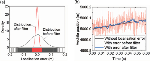
When two trains are close to each other (the second state), e.g. distance shorter than 1.0 m, auxiliary inter-train sensors such as optical sensors can be used to provide more accurate train positions. During the second state, inter-train auxiliary sensor accuracy was assumed as below 0.05 m at confidence levels above 95% per commercial product performance [Citation22].
5.2. Case study with the hyperbolic tangent gap reference
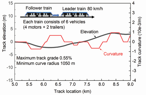
Two simulations were first conducted by using the hyperbolic tangent function as the transitional gap references to study a coupling and a decoupling process. The simulated railway track is shown in . Both simulations started with the first vehicle of the leader train located at 5.0 km track location. The ATO algorithm kept the leader train speed at 80 km/h; it used a jerk limit of 0.9 m/s3 and an acceleration limit of 1.5 m/s2 with the consideration of passenger comfort. The coupling simulation was conducted with s (see EquationEquation (5)
(5)
(5) ) and
s for the decoupling simulation; the starting reference gap for the coupling simulation and the final reference gap for the decoupling simulation were the same and set as 34 m.
Figure 8. Simulated track information.
It is also noted that, during a normal Automatic Coupling process, a small impact speed (0.5–1.0 km/h) is required to open the spring mechanism in the DAC to allow coupling. However, during Dynamic Coupling, minimum impact is desirable. Therefore, it is proposed to use the pneumatic uncoupling cylinder to keep the DAC open during the coupling process, to therefore allow coupling with zero impact speed. However, considering that the hyperbolic tangent function has a very slow changing rate after 100 s as shown in , to reasonably speed up the coupling process without causing safety risks, the dynamic gap was set to be 5 mm shorter than the designed hyperbolic tangent function. In other words, the reference gap used for the controller at the coupling instant was -5 mm. This negative reference gap was called negative Reference Gap at Coupling Instant (RG@CI) in this paper. The negative RG@CI also helps to ensure successful coupling of two trains as the controller cannot constantly maintain the gap to its theoretical value and the system also experiences external disturbances, such as resistance forces and gradient forces.
Similarly, considering the external disturbances, at the decoupling instant, a positive Reference Gap at Decoupling Instant (RG@DI) was used to get the follower trains quickly detached from the leader train. In the first decoupling simulation, RG@DI = 1 mm was used, which means at the decoupling instant the reference gap for the controller was 1 mm.
Per existing experience obtained from high-speed train DAC systems, there is a limit in terms of track radius to allow successful automatic coupling of two trains. From discussions with high-speed train engineers, minimum track radius was recommended to be greater than 1000 m. Track radii in were then set to have a minimum value of 1050 m.
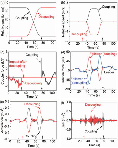
Simulation results are shown in . In this figure, the black arrow on the horizontal axis marks the time point when two end couplers are first in contact, which indicates the end of the coupling process. The red arrow on the horizontal axis marks the time point when two end couplers are first detached from each other, which indicates the start of the decoupling process. show the relative positions and speeds, respectively, between the leader train and the follower train during the coupling and decoupling processes. The results show that the simulated train movements well matched the designed gap reference designed in Section 3.
Figure 9. Dynamic coupling simulation results of the hyperbolic tangent case: (a) relative train position, (b) relative train speed, (c) coupler force at the end couplers, (d) train T/B forces, (e) longitudinal acceleration of the first vehicle of the follower train, and (f) longitudinal jerk of the first vehicle of the follower train. Note: the black and red arrows on the horizontal axis indicate the coupling and decoupling time points, respectively.
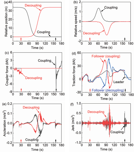
shows the end coupler force during the coupling and decoupling processes. Results show that the maximum coupler forces were less than 10 kN during the Dynamic Coupling. shows the T/B forces simulated for each train. The sign convention was set to be that traction forces with positive values whilst brake forces were negative values. It is noted that T/B forces of the leader train were also used for the follower train when the two trains were coupled together. show the simulated longitudinal acceleration and jerk, respectively, for the first vehicle of the follower train. The results of this vehicle were selected for presentations as the simulations show that the vehicle at this position usually has highest longitudinal acceleration and jerk during the coupling and decoupling processes. The results show that the simulated Dynamic Coupling was conducted smoothly; maximum longitudinal accelerations for the coupling and decoupling processes were 0.14 and 0.13 m/s2, respectively; maximum jerks were 0.70 and 0.97 m/s3, respectively. It is also noted that these maximum values were not recorded near coupling and decoupling timepoints (marked by the arrows). Maximum longitudinal accelerations simulated within 10 s after the coupling and decoupling points were both 0.05 m/s2. Maximum longitudinal jerks simulated within 10 s after the coupling and decoupling points were 0.60 and 0.37 m/s3, respectively.
To investigate the influences of RG@CI on system performance near the coupling instant, five coupling simulations with different RG@CI were conducted as listed in . The longest RG@CI was -10 mm; it was acceptable for DAC systems. As shown in , a pair of DAC allows up to 100 mm deflections. The results show that coupling time was almost the same when RG@CI was not longer than -5.0 mm (157–158 s). When RG@CI was longer than -5.0 mm, the coupling time was evidently reduced to 150 s (RG@CI = -7.5 mm) and 144 s (RG@CI = -10.0 mm). From 0.0 to -5.0 mm, maximum acceleration and maximum jerk generally increased with the increase of RG@CI. However, these two parameters significantly reduced when RG@CI was -7.5 and 10.0 mm. The time history of coupler forces of the RG@CI = -5.0 mm and RG@CI =-7.5 mm cases are shown in . The RG@CI =-7.5 mm case did not show evident train-to-train impact and therefore the coupler force was smaller. The reason behind the difference was mainly related track locations and had a certain level of randomness generated from external disturbances. This phenomenon remains as a future research topic that requires discussions of a separated publication.
Figure 10. Coupler force examples at coupling and decoupling.
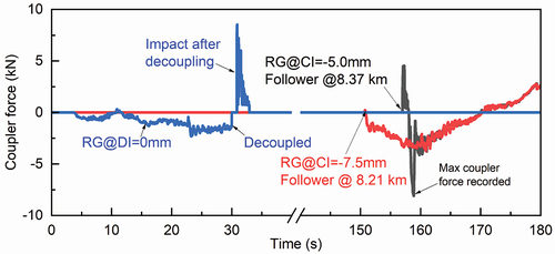
Table 3. System performance near the coupling instant (tanh =hyperbolic tangent, exp=exponential).
shows the influences of RG@DI on system performance. Results indicate that when RG@DI = 0 mm, a decoupling impact was recorded as shown in . The follower train was decoupled from the leader train first. However, due to external disturbances, the follower train ran into the leader train once more and generated a decoupling impact. The decoupling impact had a maximum coupler force of 8.5 kN and caused a maximum jerk of 1.46 m/s3. This type of decoupling impacts should be avoided and can be avoided by increasing RG@DI as shown in . When decoupling impacts were avoided, maximum jerk during the decoupling process increased with the increase of RG@DI, which means the RG@DI should not be excessively long.
Table 4. System performance near the decoupling instant (tanh =hyperbolic tangent, exp=exponential).
5.3. Case study with the exponential gap reference
The same simulations conducted in Section 5.2 were also conducted by using the gap references generated from the exponential function. Example results for the RG@CI = -5 mm and RG@DI = 1 mm cases are shown in . The difference for the exponential case were that the coupling and decoupling process last only 50 s as shown in . The same as the hyperbolic tangent case, there were 30 s extra simulations before and after the coupling and decoupling process, therefore the simulation time in was 110 s. System performance of various cases mentioned previously is also listed in .
Figure 11. Dynamic coupling simulation results of the exponential case: (a) relative train position, (b) relative train speed, (c) coupler force at the end couplers, (d) train T/B forces, (e) longitudinal acceleration of the first vehicle of the follower train, and (f) longitudinal jerk of the first vehicle of the follower train. Note: the black and red arrows on the horizontal axis indicate the coupling and decoupling time points, respectively.
For the coupling process, the coupling time of the exponential case was evidently shorter compared with hyperbolic tangential case. When RG@CI = 0.0 mm (exponential case), the coupling time was 98 s; when RG@CI was longer than 0.0 mm, the coupling time was significantly reduced to 76–77 s. Generally, the maximum jerk increased with the increase of RG@CI in the exponential case.
For the decoupling process, decoupling impacts were recorded when RG@DI was shorter than 2 mm. Wen RG@DI = 0 mm, the decoupling impact force was 10.1 kN and the maximum jerk was 12 m/s3 which exceeded the recommended jerk limit at 0.9 m/s3 [Citation13]. Once again, the results indicated that a certain distance for RG@DI was recommended to avoid decoupling impact. Also, it was noted that not all decoupling impacts would cause excessive jerks. For example, when RG@DI = 1 mm, a decoupling impact was recorded as shown in , however, the maximum jerk recorded during the decoupling process was only 0.38 m/s3. The differences in the maximum second impact force also reflected the influences of related track locations and had a certain level of randomness generated from external disturbances. As discussed previously, this randomness feature remains as a future research topic that requires discussions of a separated publication.
Another interesting observation was that for the hyperbolic tangent case (see ) the maximum decoupling and coupling jerks were measured during the switch of accelerations between positive and negative values (around 100 s). However, the maximum coupling jerk during the exponential case (see ) was recorded near the coupling instant. This observation reflected the advantage of placing a transition state between positive and negative acceleration as discussed while designing the transitional gap references. The exponential case also had the advantage of having shorter coupling and decoupling time, which was beneficial to reduce the track section length where required infrastructure upgrades as shown in .
6. Conclusions
The emerging Dynamic Coupling technology allows trains to be coupled and decoupled at cruising speeds. It is based on the Virtual Coupling technology and is more challenging for coupler designs, train control and communication technologies, but Dynamic Coupling requires much less investment for infrastructure. So far, Dynamic Coupling has not yet been systematically studied. This paper focused on the simulations of train control and dynamics of Dynamic Coupling.
First, a Dynamic Coupling controller based on an adaptive Virtual Coupling controller was introduced. Compared with the Virtual Coupling application, the final gap reference in Dynamic Coupling was zero. Second, two transitional gap references were designed based on a hyperbolic tangent function and an exponential function. The transitional gap references guided the movements of the follower train to achieve coupling and decoupling. Third, a 2D train model was presented and simulated by using a parallel computing scheme. Each individual vehicle of the simulated trains was simulated by an independent computer core. Finally, case studies by using two different transitional gap references were conducted to simulate the Dynamic Coupling process of a passenger train at the speed of 80 km/h.
The results indicated that a certain RG@CI was recommended (e.g. -5 mm) to ensure successful and quick coupling process; however, the RG@CI should not be too large as train-to-train impacts generally increased with the increase of RG@CI. A certain RG@DI was also recommended (e.g. 2 mm) to avoid impact during the decoupling process. Decoupling impact have caused train longitudinal jerk higher than comfort limits. In the meantime, the RG@DI should not be too large as maximum jerk generally increased with the increases of RG@DI.
Comparatively, the exponential case had shorter coupling and decoupling time, which was beneficial to reduce the track section length where required infrastructure upgrades. The exponential case also had a meaningful transition state between the switch of positive and negative accelerations, which was beneficial to achieve lower train longitudinal jerk.
Two simulation cases (RG@DI = 0 and 4 mm) had maximum jerks exceeded the recommended comfort limit (0.9 m/s3); all other cases had acceptable longitudinal accelerations and jerks. The simulated train movements well matched the designed transitional gap references, Dynamic Coupling was possible in terms of train dynamics in the simulated cases.
Acknowledgments
Dr Qing Wu is the recipient of an Australian Research Council Discovery Early Career Award (project number DE210100273) funded by the Australian Government. The editing contribution of Mr. Tim McSweeney (Adjunct Research Fellow, Centre for Railway Engineering) is gratefully acknowledged.
Disclosure statement
No potential conflict of interest was reported by the author(s).
References
- Nold M, Corman F. Dynamic train unit coupling and decoupling at cruising speed: systematic classification, operational potentials, and research agenda. J Rail Trans Plan Manag. 2021;18:article 100241. DOI:10.1016/j.jrtpm.2021.100241
- Wagner S, Cole C, Spiryagin M. A review on design and testing methodologies of modern freight train draft gear system. Rail Eng Sci. 2021;29(2):127–151.
- Goverde R. Application roadmap for the introduction of virtual coupling. Brussels Belgium: SHIFT2RAIL; 2020.
- Park J, Lee B, Eun Y. Virtual coupling of railway vehicles: gap reference for merge and separation, robust control, and position measurement. IEEE Trans Intell Transp Syst. 2022;23(2):1085–1096. DOI:10.1109/TITS.2020.3019979
- Liu Y, Ou D, Yang Y, et al. A method for maintaining virtually coupled states of train convoys. Proceedings of the Institution of Mechanical Engineers, Part F: Journal of Rail and Rapid Transit; 2022 June. DOI:10.1177/09544097221103333
- Liu Y, Zhou Y, Su S, et al. An analytical optimal control approach for virtually coupled high-speed trains with local and string stability. Transp Res Part C. 2021;125:article 102886.
- Wu Q, Ge X, Han QL, et al. Dynamics and control simulation of railway virtual coupling. Veh Syst Dyn. 2022:1–25. DOI:10.1080/00423114.2022.2105241
- Aoun J, Quaglietta E, Goverde R. Potential and challenges of virtual coupling for train platooning. Presentation at RailTech Europe Live 21 Virtual Conference; 2021.
- Ge X, Han QL, Wu Q, et al. Resilient and safe platooning control of connected automated vehicles against intermittent denial-of-service attacks. IEEE/CAA Journal of Automatica Sinica; 2022. DOI:10.1109/JAS.2022.10584
- Ersal T, Kolmanovsky I, Masoud N, et al. Connected and automated road vehicles: state of the art and future challenges. Veh Syst Dyn. 2020;58(5):672–704. DOI:10.1080/00423114.2020.1741652
- Hassanain O, Alirezaei M, Ploeg J, et al. String-stable automated steering in cooperative driving applications. Veh Syst Dyn. 2020;58(5):826–842. DOI:10.1080/00423114.2020.1749288
- Ge X, Han QL, Wang J, et al. Scalable and resilient platooning control of cooperative automated vehicles. IEEE Trans Veh Technol. 2022;71(4):3595–3608. DOI:10.1109/TVT.2022.3147371
- Bae I, Moon J, Seo J. Toward a comfortable driving experience for a self-driving shuttle bus. Electron. 2019;8(941):1–13.
- Iwnicki S, Spiryagin M, Cole C, et al. Handbook of railway vehicle dynamics. New York: CRC Press; 2019.
- Fu B, Giossi R, Persson R, et al. Active suspension in railway vehicles: a literature survey. Rail Eng Sci. 2020;28(1):3–35.
- Wu Q, Cole C, Spiryagin M. Parallel computing enables whole-trip train dynamics optimizations. ASME J Comput Nonlinear Dynam. 2016;11(4):044503.
- Barney B. Message passing interface (MPI) [Internet]. Livermore (CA): Lawrence Livermore National Laboratory; 2022 [cited 2022 Dec 1]. Available at https://hpc-tutorials.llnl.gov/mpi/
- Wu Q, Sun Y, Spiryagin M, et al. Parallel co-simulation method for railway vehicle-track dynamics. ASME J Comput Nonlinear Dynam. 2018;13(4):041004.
- Ibrahim R, Stephan S, Fabian D. Proceedings of the ITS-G5 challenges and 5G solutions for vehicular platooning; Kassel, Germany; 2016.
- Rehrl K, Gröchenig S. Evaluating localization accuracy of automated driving systems. Sensors. 2021;21(17):5855. DOI:10.3390/s21175855
- Sessa P, De Martinis V, Corman F. Filtering approaches for online train motion estimation with onboard power measurements. Comput-Aided Civil Infrastruct Eng. 2020;35(5):415–429.
- Spartfun. Distance sensor comparison guide. 2022 [cited 2022 Dec 1]. Available at https://www.sparkfun.com/distance_sensor_comparison_guide