Travel times in quasi-dynamic traffic assignment

ABSTRACT

By extending static traffic assignment with explicit capacity constraints, quasi-dynamic traffic assignment yields more realistic results while avoiding many disadvantages of a dynamic assignment. We analyse the computation of travel times in quasi-dynamic assignment models. We formulate and check requirements for the correctness of resulting travel times, addressing both the calculation of travel times for individual routes and links itself, as well as the differences between travel times of different travel choices. We demonstrate that existing approaches for travel time computation in the literature fail to satisfy all requirements and derive a new link travel time formula from the vertical queuing theory that does meet all requirements. We discuss expected changes to assignment results and methodological advantages for pathfinding and model extensions, including horizontal queuing. The new link travel time formulation is finally applied to three example scenarios from literature.

KEYWORDS:

• Quasi-dynamic traffic assignment
• link travel time
• vertical queuing theory
• capacity constraint
• link performance function

1. Introduction

There is a long tradition of static traffic assignment (STA) in transportation research. Albeit dynamic traffic assignment (DTA) can yield more detailed and realistic results, it unfortunately also comes with greater model complexity, higher computational costs, higher data requirements, and poorer convergence. And hence, STA is still much used in practice and research. The most important limitation of traditional STA models is the lack of explicit capacity constraints, which results in errors in the modelled congestion patterns around bottlenecks, and consequently also errors in travel times and delays. To remedy this, Bakker, Mijjer, and Hofman (1994), Bifulco and Crisalli (1998), Lam and Zhang (2000), Bundschuh, Vortisch, and Van Vuuren (2006), and Gentile, Velonà, and Cantarella (2014) formulated capacity-constrained STA models where excess traffic at bottlenecks can accumulate in residual queues. These queues are initially empty and absorb whatever traffic demand from the studied time period that exceeds capacity. Hence, while in traditional STA based on link performance functions (Bureau of Public Roads 1964) traffic is omnipresent, instead in capacity-constrained STA traffic is instantaneously propagated over its entire route, but the fraction of a route’s demand ending up in a residual queue is not propagated over the remainder of that route.

Bliemer et al. (2014) refer to this as quasi-dynamic traffic assignment (QDTA), and formulate the capacity-constrained traffic propagation and assignment as two fixed-point problems, including calculation of route travel times. Their formulation supports use of generic first-order node models (Tampère et al. 2011), and correctly places vertical queues in front of bottleneck nodes. Brederode et al. (2019) supplement the approach with an additional horizontal queuing calculation to account for spillback and interaction effects between bottlenecks, based on a dynamic model (Raadsen, Bliemer, and Bell 2016). Raadsen and Bliemer (2018) instead integrate spillback and bottleneck interactions directly into the original flow propagation model. Nakayama and Connors (2014) formulate a variation of QDTA where the residual queues are transferred to the next time period.

Within the context of QDTA, this paper focuses specifically on the computation of travel times, while we discuss the propagation of traffic through the network to the extent relevant. To this end, we formulate a list of requirements shown in Table 1 that can be divided into two categories:

• requirements for absolute correctness that ensure a valid composition of the travel time calculation for individual routes and links (I-III);

• requirements for relative correctness that ensure a valid comparison between travel times of alternative routes or alternative demand patterns (IV-VI).

Table 1. Satisfaction of requirements for travel time calculation by various traffic assignment methods^a.

^aThis comparison focuses on the calculation of travel times. Advances in the flow propagation model are not shown here. For Nakayama and Connors (2014) it is assumed flow propagation is based on capacity constraints.

The six requirements are listed here for reference and will be introduced and discussed throughout this paper. Correctness here refers to the consistency with reality and traffic flow theory. The requirements can be summarised as follows:

1. Corridor Compatibility: travel times on a corridor network are compatible with queuing theory calculations;

2. Route is Sum of Links: the travel time of a route equals the sum of travel times of the links along the route;

3. Steady State Consistency: link travel times are based on both instantaneous traffic propagation and homogeneous traffic composition, or on neither;

4. Correct Derivatives: in case of a link with a fixed exit capacity, the partial derivatives of the link’s travel time with respect to both the link’s demand and the link’s flow have the correct sign;

5. First-In-First-Out: route travel times respect the first-in-first-out property of links: it is not possible to leave a link earlier by entering it later;

6. Stops have No Effect: insertion of intermediate stops in a route cannot change the route’s travel time (other than the time spent stopped).

The requirements are specified in more detail later in this paper. As will be shown, all requirements are satisfied by DTA, while QDTA formulations until now violate several requirements. This is solved in this paper where we present a new procedure to correctly compute travel times. Table 1 presents an overview of what model types satisfy which requirements.

In this paper, we show that the existing QDTA travel time computation procedures fail to meet requirements for both absolute and relative correctness. Our main contribution is a new QDTA travel time formula derived from queuing theory that does satisfy all requirements and can readily replace the Bliemer et al. (2014) formula. We also analyse what this formula replacement implies for assignment results and pathfinding, and illustrate how horizontal queuing and other extensions can be incorporated. Note that our new travel time formula can be used in combination with existing flow propagation models from Bliemer et al. (2014) and Raadsen and Bliemer (2018), so we will not discuss QDTA flow propagation in detail.

The structure of this paper is as follows. First, Section 2 revisits the derivation of quasi-dynamic travel time formulas from queuing theory, resulting in our new QDTA travel time formula. Requirements for absolute correctness are formulated and investigated in the process. Then, Section 3 formulates and investigates requirements for relative correctness, by considering derivatives of the link travel time and analysing route travel times in an example network. Section 4 analyses further implications of using our new formula for assignment results and pathfinding with congested travel times, and shows how it can be further extended with horizontal queuing and other improvements. Section 5 applies our new travel time formula to three example scenarios from literature. Finally, Section 6 summarises our conclusions.

2. Theoretical derivation of quasi-dynamic travel times

In this section, we will derive a formula for the travel time ${\tau }_a$ of link $a$. Like Bliemer et al. (2014, 371), we split the travel time into a free-flow travel time ${\tau }_a^{\mathrm{ff}}$ and a queuing delay ${\tau }_a^{\mathrm{q}\mathrm{u}\mathrm{e}\mathrm{u}\mathrm{e}}$: (1) ${\tau }_a={\tau }_a^{\mathrm{ff}}+{\tau }_a^{\mathrm{q}\mathrm{u}\mathrm{e}\mathrm{u}\mathrm{e}}.$(1) Here, ${\tau }_a^{\mathrm{ff}}$ is either a constant or an increasing function of link inflow $q_a$. Bakker, Mijjer, and Hofman (1994, 320), Lam and Zhang (2000, 123), Gentile, Velonà, and Cantarella (2014, 322), and Brederode et al. (2019, 7) suggest the latter. Nevertheless, our focus is on deriving a formula for ${\tau }_a^{\mathrm{q}\mathrm{u}\mathrm{e}\mathrm{u}\mathrm{e}}$ that indicates the extra travel time due to the link’s exit capacity being exceeded and the consequent queue being formed on the link. The formula for this queuing delay needs be consistent with the arrival and service rates of traffic, also in networks with more than one bottleneck.

QDTA models traffic flows in a single time period, and unlike DTA does not distinguish any departure times. Therefore, the (link and route) travel times in our computations are static, and hence there is no time index. The traffic flow propagation component of any QDTA model is set up such that all traffic demand either reaches their destination or accumulates in residual queues. Either way, we seek to estimate the travel time of an entire route. If the route is long, congested, or both, these route travel times may exceed the duration of the simulated time period (similar to STA).

Note that Nakayama and Connors (2014) deviate from the above definition of QDTA by modelling multiple time periods, and are closer to traditional DTA with large time steps. Their flow propagation is also not necessarily based on capacity constraints. To ensure a proper comparison with other QDTA models, we assume it is.

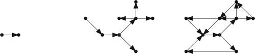
This section derives the link travel time formula for increasingly complex networks: a single link in Section 2.1, a diverges-only network in Section 2.2, and a general network in Section 2.3 (Figure 1). The main contribution is the general network formula presented in Section 2.3, which is an improvement of the Bliemer et al. (2014) formula. In order to derive it, we analyse the simpler networks first. A second contribution is the requirements for absolute correctness that are formulated during its derivation.

Figure 1. Network types: single-link network (left), diverges-only network (middle), general network (right).

2.1. Single link

We first consider a network consisting of a single link $a$, subject to a constant traffic demand rate $f_a$ departing during time period $\left[0,T\right]$. Since there are no upstream queues, the link inflow $q_a$ is equal to the demand rate $f_a$. A queue may, however, build up at the exit of the link, consisting of traffic waiting to traverse the next node, due to insufficient capacity as determined by the node model. Let ${\alpha }_a\in \left(0,1\right]$ be the link flow reduction factor, such that the link outflow is ${\alpha }_a{q}_a$. Initially, at time $0$, there is no queue on the link. Because traffic propagation is instantaneous, a queue forms ‘immediately’. At the end of the study time period, the number of vehicles in the queue is (Bliemer et al. 2014, 371) (2) $Q_a=q_{a}T-{\alpha }_a{q}_{a}T=\left(1-{\alpha }_a\right)q_{a}T.$(2) Assuming the link outflow remains ${\alpha }_a{q}_a$ after $T$ until all vehicles left, the last vehicle to enter the queue has to wait (3) $\frac{Q_a}{{\alpha }_a{q}_a}=\frac{1-{\alpha }_a}{{\alpha }_a}T=\left(\frac{1}{{\alpha }_a}-1\right)T$(3) time for the queue to dissolve before it can exit the link. Since the queue grew linearly from $0$ to $Q_a$, the average delay for all $f_{a}T=q_{a}T$ vehicles equals half of this (Bliemer et al. 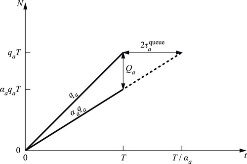2014, 371; Gentile, Velonà, and Cantarella 2014, 319): (4) ${\tau }_a^{\mathrm{q}\mathrm{u}\mathrm{e}\mathrm{u}\mathrm{e}}=\left(\frac{1}{{\alpha }_a}-1\right)\frac{T}{2}.$(4) The build-up of the link’s queue over time is depicted in Figure 2 using cumulative curves. Because of the first-in-first-out property, the horizontal distance between the entrance and exit curves represents the delay of the $N$th vehicle. This shows visually how the above formulas are derived.

Figure 2. Cumulative numbers of vehicles entering and exiting the queue over time, on a single link network.

2.2. Diverges-only network

Now consider a link $a$ that is part of a corridor network consisting of multiple links, where all nodes are either one-to-one nodes or diverges. The link inflow $q_a$ during time period $\left[0,T\right]$ may now be constrained by queues in the set of links ${\eta }_a$ upstream of link $a$ (excluding itself, $a\notin {\eta }_a$). More precisely (Bifulco and Crisalli 1998, 88; Bliemer et al. 2014, 369): (5) $q_a=f_a\prod _{a^{\mathrm{\prime }}\in {\eta }_a}{\alpha }_{a^{\mathrm{\prime }}}.$(5) Thus traffic will keep flowing into the queue at the exit of link $a$ after time period $\left[0,T\right]$ ended. We again assume the link outflow remains ${\alpha }_a{q}_a$ until all vehicles left. This implies inflows into following links will also remain constant. Because both the inflow and outflow of link $a$ remain constant after $\left[0,T\right]$ until the last vehicle enters/exits the link, therefore the last vehicle enters the queue on link $a$ at time ${\overline{T}}_a$ such that the full link demand is processed, i.e. (6) $q_a{\overline{T}}_a=f_{a}T,$(6) so (7) ${\overline{T}}_a=\frac{f_a}{q_a}T=\frac{1}{\prod _{a^{\mathrm{\prime }}\in {\eta }_a}{\alpha }_{a^{\mathrm{\prime }}}}T.$(7) At time ${\overline{T}}_a$, the number of vehicles in the queue equals (8) ${\overline{Q}}_a=q_a{\overline{T}}_a-{\alpha }_a{q}_a{\overline{T}}_a=\left(1-{\alpha }_a\right)q_a{\overline{T}}_a=\frac{1-{\alpha }_a}{\prod _{a^{\mathrm{\prime }}\in {\eta }_a}{\alpha }_{a^{\mathrm{\prime }}}}{q}_{a}T.$(8) The last vehicle thus experiences a delay of (9) $\frac{{\overline{Q}}_a}{{\alpha }_a{q}_a}=\frac{1-{\alpha }_a}{{\alpha }_a\prod _{a^{\mathrm{\prime }}\in {\eta }_a}{\alpha }_{a^{\mathrm{\prime }}}}T=\frac{1}{\prod _{a^{\mathrm{\prime }}\in {\eta }_a}{\alpha }_{a^{\mathrm{\prime }}}}\left(\frac{1}{{\alpha }_a}-1\right)T.$(9) The average delay on the link for all $f_{a}T$ vehicles, therefore, equals half of this (Bliemer et al. 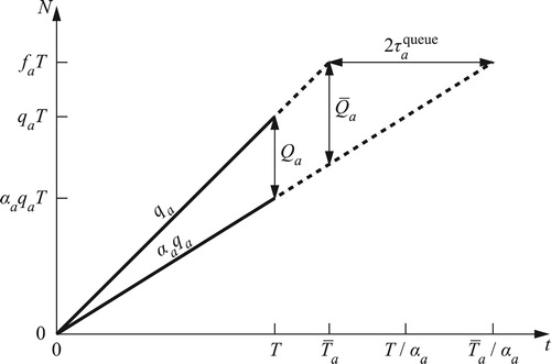2014, 372): (10) ${\tau }_a^{\mathrm{q}\mathrm{u}\mathrm{e}\mathrm{u}\mathrm{e}}=\frac{1}{\prod _{a^{\mathrm{\prime }}\in {\eta }_a}{\alpha }_{a^{\mathrm{\prime }}}}\left(\frac{1}{{\alpha }_a}-1\right)\frac{T}{2}.$(10) Figure 3 depicts the queue build-up in terms of cumulative numbers of vehicles over time.

Figure 3. Cumulative numbers of vehicles entering and exiting a link’s queue over time, in a network with multiple links.

The total average delay of link $a$ and all links before it equals (Bliemer et al. 2014, 372) (11) $\begin{array}{rl}\sum _{a^{\mathrm{\prime }}\in {\eta }_a\cup \left\{a\right\}}{\tau }_{a^{\mathrm{\prime }}}^{\mathrm{q}\mathrm{u}\mathrm{e}\mathrm{u}\mathrm{e}}& =\sum _{a^{\mathrm{\prime }}\in {\eta }_a\cup \left\{a\right\}}\frac{1}{\prod _{a^{\mathrm{\prime }\mathrm{\prime }}\in {\eta }_{a^{\mathrm{\prime }}}}{\alpha }_{a^{\mathrm{\prime }\mathrm{\prime }}}}\left(\frac{1}{{\alpha }_{a^{\mathrm{\prime }}}}-1\right)\frac{T}{2}\\ & =\sum _{a^{\mathrm{\prime }}\in {\eta }_a\cup \left\{a\right\}}\left(\frac{1}{\prod _{a^{\mathrm{\prime }\mathrm{\prime }}\in {\eta }_{a^{\mathrm{\prime }}}\cup \left\{a^{\mathrm{\prime }}\right\}}{\alpha }_{a^{\mathrm{\prime }\mathrm{\prime }}}}-\frac{1}{\prod _{a^{\mathrm{\prime }\mathrm{\prime }}\in {\eta }_{a^{\mathrm{\prime }}}}{\alpha }_{a^{\mathrm{\prime }\mathrm{\prime }}}}\right)\frac{T}{2}=\left(\frac{1}{\prod _{a^{\mathrm{\prime }}\in {\eta }_a\cup \left\{a\right\}}{\alpha }_{a^{\mathrm{\prime }}}}-1\right)\frac{T}{2}.\end{array}$(11) As discovered by Bliemer et al. (2014, 371–372), this is consistent with the vertical queuing theory on a corridor: the queuing delay of a series of consecutive bottlenecks is equal to the queuing delay of a single bottleneck with severities multiplied. It thereby satisfies our first requirement in Table 1.

Requirement I. (Corridor Compatibility):

Travel times on a corridor network are compatible with queuing theory calculations with the corridor inflow as arrival rate and the final link outflow as service rate. Depending on the capabilities of the traffic propagation model, either vertical queuing or horizontal queuing may be used.

The dynamic modelling step of Brederode et al. (2019) correctly models horizontal queuing on a corridor network and therefore satisfies this requirement. Albeit with vertical queuing only, Bundschuh, Vortisch, and Van Vuuren (2006) similarly use a dynamic modelling step to account for interactions between bottlenecks, thus also satisfying Requirement I. Bakker, Mijjer, and Hofman (1994) and Lam and Zhang (2000) do not account for such interactions. Gentile, Velonà, and Cantarella (2014, 322) recognise the problem with multiple bottlenecks in a corridor, but do not develop a general solution like Equation (10). Nakayama and Connors (2014) transfer the residual queue to a new time period which will have a smaller delay, violating Requirement I. STA fails Requirement I because the link performance functions do not capture flow metering due to capacity constraints and hence do not model queue build-up and its effect on downstream links.

2.3. General network

We now proceed to calculating travel times in general networks. In a network with merging traffic, the traffic flow rate and the composition of traffic after a merge may vary. Hence the calculation of delays in general networks is a bit more involved. While Bliemer et al. (2014, 372) immediately infer the corridor result to also hold for general networks, we follow a more rigorous derivation.

We can convert a general network into a diverge-only network by replacing links after merges with multiple parallel links, and assigning flows to the parallel links in such a way that traffic flows never merge. Let $P_a$ be the set of parallel links that replace link $a$: (12) $\begin{array}{rl}\sum _{p\in P_a}{f}_p& =f_a,\\ \sum _{p\in P_a}{q}_p& =q_a.\end{array}$(12) Each parallel link $p\in P_a$ now has a well-defined set of predecessor links ${\eta }_p$. Using the same reasoning as for the diverge-only network, we can compute the average delay on any link $p\in P_a$: (13) $\mathrm{\forall }p\in P_a:{\tau }_p^{\mathrm{q}\mathrm{u}\mathrm{e}\mathrm{u}\mathrm{e}}=\frac{1}{\prod _{p^{\mathrm{\prime }}\in {\eta }_p}{\alpha }_{p^{\mathrm{\prime }}}}\left(\frac{1}{{\alpha }_p}-1\right)\frac{T}{2}=\frac{f_p}{q_p}\left(\frac{1}{{\alpha }_p}-1\right)\frac{T}{2}.$(13)

To preserve the composition of inflow into the node downstream of any original link $a^{\mathrm{\prime }}$, including conservation of turning fractions (Daganzo 1995, 88; Tampère et al. 2011, 295), we require (14) $\mathrm{\forall }{p}^{\mathrm{\prime }}\in P_{a^{\mathrm{\prime }}}:{\alpha }_{p^{\mathrm{\prime }}}={\alpha }_{a^{\mathrm{\prime }}},$(14) resulting in (15) $\mathrm{\forall }p\in P_a:{\tau }_p^{\mathrm{q}\mathrm{u}\mathrm{e}\mathrm{u}\mathrm{e}}=\frac{1}{\prod _{p^{\mathrm{\prime }}\in {\eta }_p}{\alpha }_{p^{\mathrm{\prime }}}}\left(\frac{1}{{\alpha }_a}-1\right)\frac{T}{2}=\frac{f_p}{q_p}\left(\frac{1}{{\alpha }_a}-1\right)\frac{T}{2}.$(15)

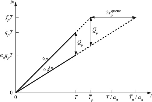
The derivation is depicted in Figure 4. The difference with Figure 3 is that a separate travel time ${\tau }_p^{\mathrm{q}\mathrm{u}\mathrm{e}\mathrm{u}\mathrm{e}}$ is calculated for each parallel link $p\in P_a$ representing a portion of the real link’s traffic.

Figure 4. Cumulative numbers of vehicles entering and exiting the queue of one of the parallel links over time.

Equation (15) matches the final result reported by Bliemer et al. (2014, 372). Even though the links $p\in P_a$ now have equal outflow-to-inflow ratios ${\alpha }_a$, they still have separate queues with potentially different delays. Original link $a$ does not yet have a unique travel time: instead, the travel time one experiences still varies depending on what predecessor links they came from, i.e. traffic following different routes experience different travel times on the same physical link. Because this difference cannot be attributed to differences in departure time or total prior travel time, the following requirement in Table 1 is not met:

Requirement II. (Route is Sum of Links):

The travel time of a route equals the sum of travel times of the links along the route. The travel time traffic experiences on a link may vary with the time the traffic enters the link, but not with where the traffic originates from.

For Nakayama and Connors (2014), link travel time also varies for different users of the link in violation of this requirement. All other QDTA methods in Table 1 satisfy Requirement II, as well as traditional STA.

In order to satisfy Requirement II, we continue our derivation by merging the parallel links $p\in P_a$ back into a single link $a$ with a single travel time ${\tau }_a$. Naïve summation of the time-dependent inflows and outflows of links $p\in P_a$ may lead to non-constant inflow and outflow for link $a$, because according to Equation (7), the summed inflows $q_p$ can have different durations ${\overline{T}}_p$ and the summed outflows ${\alpha }_a{q}_p$ can have different durations ${\overline{T}}_p/{\alpha }_a$. This is also problematic, because it violates the stationarity of the traffic composition implied by the instantaneous propagation of flows. Because the instantaneous flow propagation does not take travel times into account, it is impossible to conclude from the flow profiles that traffic from one origin arrives on average earlier at some point than the other traffic. Within quasi-dynamic modelling, the only way to avoid implying such conclusions is to assume a constant inflow for link $a$ in which the separate contributions of different origins can no longer be identified.¹ This leads to the next requirement:

Requirement III. (Steady State Consistency):

Link travel times are based on both instantaneous traffic propagation and homogeneous traffic composition, or on neither. Put differently, either traffic propagation and demand both are time-dependent, or both are in steady state.

Despite violating Requirement III, the idea of summing the cumulative inflow and outflow curves is further explored in the Appendix, which reveals another significant problem discussed later in Section 3.1. Bundschuh, Vortisch, and Van Vuuren (2006) and Brederode et al. (2019) propose a different approach that restricts instantaneous flow propagation to unconstrained flows only, using an additional dynamic network modelling phase interaction effects between bottlenecks, and in case of Brederode et al. (2019) also horizontal queue build-up and spillback. This means link inflows and outflows are not constant, but vary over a virtual time scale, referred to as queuing time, and travel times are calculated using the resulting piecewise-linear cumulative inflow and outflow curves. Naturally, the non-linearity of these curves also violates Requirement III. Nakayama and Connors (2014) suffer from the same problem.

Below we continue by seeking to construct a homogenous constant inflow profile for link $a$ that is consistent with the inflow profiles of links $p\in P_a$. The inflow rate $q_a$ is already given by Equation (12). To preserve the total inflow, the duration ${\overline{T}}_a$ is then the average of durations ${\overline{T}}_p$ weighted with inflow rates $q_p$. Substituting Equation (7), this weighted average simplifies to (16) ${\overline{T}}_a=\sum _{p\in P_a}\frac{q_p}{q_a}{\overline{T}}_p=\sum _{p\in P_a}\frac{q_p}{q_a}\frac{f_p}{q_p}T=\sum _{p\in P_a}\frac{f_p}{q_a}T=\frac{f_a}{q_a}T.$(16) Now that we made the link inflow constant, the link outflow is also constant. The number of vehicles in the combined queue on link $a$ at time ${\overline{T}}_a$ therefore equals (17) ${\overline{Q}}_a=q_a{\overline{T}}_a-{\alpha }_a{q}_a{\overline{T}}_a=\left(1-{\alpha }_a\right)q_a{\overline{T}}_a=\left(1-{\alpha }_a\right)q_a\frac{f_a}{q_a}T=\left(1-{\alpha }_a\right)f_{a}T.$(17) The delay of the last vehicle is therefore (18) $\frac{{\overline{Q}}_a}{{\alpha }_a{q}_a}=\frac{\left(1-{\alpha }_a\right)f_{a}T}{{\alpha }_a{q}_a}=\frac{f_a}{q_a}\left(\frac{1}{{\alpha }_a}-1\right)T$(18) such that the average delay is (19) ${\tau }_a^{\mathrm{q}\mathrm{u}\mathrm{e}\mathrm{u}\mathrm{e}}=\frac{f_a}{q_a}\left(\frac{1}{{\alpha }_a}-1\right)\frac{T}{2}.$(19) This result is fully consistent with the previous result for a diverges-only network. The evolution of the cumulative numbers of vehicles entering and exiting the combined queue is the same as Figure 3. The critical difference with Equation (15) is that this travel time only depends on the total demand $f_a$ and the total flow $q_a$ on the link, instead of on a specific demand component $f_p$ and flow component $q_p$ corresponding to a particular origin. The travel time is therefore now the same for all traffic on the link regardless of origin.

3. Relative correctness of quasi-dynamic travel times

Now that we have derived a travel time formula for links in a general network, we proceed to assess the relative correctness of travel times in QDTA, i.e. the ability to compare route travel times. This section is split into two parts. First, we look at the derivatives of the link travel time formula while keeping the link exit capacity fixed. Second, we check the behavioural incentives for travel choices in an example network.

3.1. Link with fixed exit capacity

We now study a link with a fixed exit capacity. Because of the invariance principle (Lebacque and Khoshyaran 2005, 370–371), this occurs when the turning fractions and competing flows at its downstream node remain constant, even in advanced first-order node models (Tampère et al. 2011, 295). Assuming link $a$ has fixed exit capacity $C_a$, we have (Bifulco and Crisalli 1998, 88) (20) ${\alpha }_a=min\left(1,\frac{C_a}{q_a}\right).$(20) Combining this with Equations (1) and (19) yields the following link travel time: (21) ${\tau }_a=\left\{\begin{array}{ll}{\tau }_a^{\mathrm{ff}}& \text{if }{q}_a\le C_a,\\ {\tau }_a^{\mathrm{ff}}+\left(\frac{f_a}{C_a}-\frac{f_a}{q_a}\right)\frac{T}{2}& \text{if }{q}_a\ge C_a.\end{array}\right.$(21) This structure of this formulation is comparable to link travel time functions in the static assignment, for example, the well-known Bureau of Public Roads (1964, p. V20) function: (22) ${\tau }_a={\tau }_a^{\mathrm{f}\mathrm{f}}\left(1+0.15{\left(\frac{f_a}{C_a}\right)}^4\right).$(22) The comparison reveals the fundamental difference that in (non-capacitated) static assignment the travel time ${\tau }_a$ only depends on the total demand $f_a$ for the link, and not also on the actual flow $q_a$ that is able to get into the link during the studied time period. (Static models don’t compute $q_a$.) Both static models and our quasi-dynamic model satisfy (23) $\left\{\begin{array}{l}\mathrm{\forall }{q}_a\in \left(0,f_a\right]:\frac{\mathrm{\partial }{\tau }_a}{\mathrm{\partial }{f}_a}\ge 0,\\ \mathrm{\forall }{q}_a\in \left(C_a,f_a\right]:\frac{\mathrm{\partial }{\tau }_a}{\mathrm{\partial }{f}_a}>0,\end{array}\right.$(23) but our quasi-dynamic model additionally satisfies (24) $\left\{\begin{array}{l}\mathrm{\forall }{q}_a\in \left(0,f_a\right]:\frac{\mathrm{\partial }{\tau }_a}{\mathrm{\partial }{q}_a}\ge 0,\\ \mathrm{\forall }{q}_a\in \left(C_a,f_a\right]:\frac{\mathrm{\partial }{\tau }_a}{\mathrm{\partial }{q}_a}>0,\end{array}\right.$(24) whereas static models always have $\mathrm{\partial }{\tau }_a/\mathrm{\partial }{q}_a=0$. Note that this also holds if ${\tau }_a^{\mathrm{f}\mathrm{f}}$ in Equation (21) is not constant but itself increases with $q_a$, as suggested at the beginning of Section 2. In conclusion, we have the following requirement:

Requirement IV. (Correct Derivatives):

In case of a link with a fixed exit capacity, the partial derivatives of the link’s travel time with respect to both the link’s demand and the link’s flow have the correct sign, in accordance with Equations (23) and (24).

If one were to derive a representative link travel time directly from Equation (15) (Bliemer et al. 2014, 372), it would be based on the total travel time of all traffic demand of all routes on the link, divided by the total traffic demand. This corresponds to the previously mentioned idea of summing the cumulative inflow and outflow curves, which was explored in the Appendix. The Appendix shows that this results in a possibility of $\mathrm{\partial }{\tau }_a/\mathrm{\partial }{f}_a<0$, violating Equation (23). The residual queue transfer to the next time period in Nakayama and Connors (2014) similarly brings down the average travel time in violation of Equation (23).

Because Bundschuh, Vortisch, and Van Vuuren (2006, 4–5) and Brederode et al. (2019, 14–15) compute ${\tau }_a^{\mathrm{q}\mathrm{u}\mathrm{e}\mathrm{u}\mathrm{e}}$ from the average distance between the piecewise-linear cumulative inflow and outflow curves. A fixed exit capacity here corresponds to a fixed maximum outflow curve that the downstream node accepts. An increase in $f_a$ can result in a decrease in ${\tau }_a^{\mathrm{q}\mathrm{u}\mathrm{e}\mathrm{u}\mathrm{e}}$ if the delay of an additional vehicle is lower than the current average delay. This again violates Equation (23).

The QDTA travel time formulas of Bakker, Mijjer, and Hofman (1994), Lam and Zhang (2000), Bundschuh, Vortisch, and Van Vuuren (2006), and Gentile, Velonà, and Cantarella (2014) are only sensitive to $q_a$ and not to $f_a$, thus also contradicting Equation (23).

3.2. Choice behaviour in example network

We will now study differences between route travel times in a simple example network, which we use to formulate two more requirements for relative correctness. Because satisfaction of Requirement II (Route is Sum of Links) automatically leads to satisfaction of the new requirements, the issues discussed below cannot occur in any model in Table 1 other than Bliemer et al. (2014) and Nakayama and Connors (2014). While our numerical example focuses on Bliemer et al. (2014), we also mention how the discovered issues affect Nakayama and Connors (2014).

To demonstrate the issues, we consider the example network from Figure 5.

Figure 5. Example network demonstrating the issues.

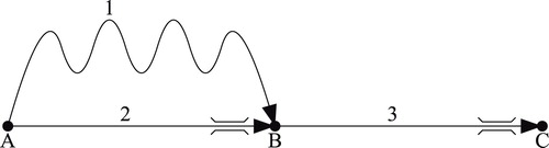
We study a time period with duration $T=60\text{min}$. The network consists of three links. Link 1 has a long free-flow travel time but is never congested, while link 2 and link 3 have a much shorter free-flow travel time, but also bottlenecks at their downstream ends with limited exit capacities $C_2$ and $C_3$²: (25) $\begin{array}{rl}& {\tau }_1^{\mathrm{ff}}=40\text{min}{C}_1=\mathrm{\infty }\\ & {\tau }_2^{\mathrm{f}\mathrm{f}}=5\text{min}{C}_2=2000\text{veh/h}\\ & {\tau }_3^{\mathrm{f}\mathrm{f}}=5\text{min}{C}_3=2250\text{veh/h}\text{.}\end{array}$(25) During the studied time period, there is traffic demand for origin-destination pairs AB and AC, and we analyse the situation where both demands split equally over the two possible routes: (26) $\begin{array}{rl}& f_{\mathrm{AB},1}=1000\text{veh/h}{f}_{\mathrm{AC},13}=3000\text{veh/h}\\ & f_{\mathrm{AB},2}=1000\text{veh/h}{f}_{\mathrm{AC},23}=3000\text{veh/h}\text{.}\end{array}$(26)

Using this information, we can solve all link inflows $q_{\cdot }$ and link flow reduction factors ${\alpha }_{\cdot }$. Normally, one would treat this as a fixed-point problem and use an algorithm like the one proposed by Bliemer et al. (2014, 376), but due to the simple structure of this example, we can find the solution directly: (27) $\begin{array}{r}\left\{\begin{array}{l}{f}_1=f_{\mathrm{AB},1}+f_{\mathrm{AC},13}=1000\text{veh/h}+3000\text{veh/h}=4000\text{veh/h}\\ q_{\mathrm{AB},1,1}=f_{\mathrm{AB},1}=1000\text{veh/h}\\ q_{\mathrm{AC},13,1}=f_{\mathrm{AC},13}=3000\text{veh/h}\\ q_1=q_{\mathrm{AB},1,1}+q_{\mathrm{AC},13,1}=1000\text{veh/h}+3000\text{veh/h}=4000\text{veh/h}\\ {\alpha }_1=min\left(1,\frac{C_1}{q_1}\right)=min\left(1,\frac{\mathrm{\infty }}{4000\text{veh/h}}\right)=1,\end{array}\right.\\ \left\{\begin{array}{l}{f}_2=f_{\mathrm{AB},2}+f_{\mathrm{AC},23}=1000\text{veh/h}+3000\text{veh/h}=4000\text{veh/h}\\ q_{\mathrm{AB},2,2}=f_{\mathrm{AB},2}=1000\text{veh/h}\\ q_{\mathrm{AC},23,2}=f_{\mathrm{AC},23}=3000\text{veh/h}\\ q_2=q_{\mathrm{AB},2,2}+q_{\mathrm{AC},23,2}=1000\text{veh/h}+3000\text{veh/h}=4000\text{veh/h}\\ {\alpha }_2=min\left(1,\frac{C_2}{q_2}\right)=min\left(1,\frac{2000\text{veh/h}}{4000\text{veh/h}}\right)=\frac{1}{2},\end{array}\right.\\ \left\{\begin{array}{l}{f}_3=f_{\mathrm{AC},13}+f_{\mathrm{AC},23}=3000\text{veh/h}+3000\text{veh/h}=6000\text{veh/h}\\ q_{\mathrm{AC},13,3}={\alpha }_1{f}_{\mathrm{AC},13}=1\cdot 3000\text{veh/h}=3000\text{veh/h}\\ q_{\mathrm{AC},23,3}={\alpha }_2{f}_{\mathrm{AC},23}=\frac{1}{2}\cdot 3000\text{veh/h}=1500\text{veh/h}\\ q_3=q_{\mathrm{AC},13,3}+q_{\mathrm{AC},23,3}=3000\text{veh/h}+1500\text{veh/h}=4500\text{veh/h}\\ {\alpha }_3=min\left(1,\frac{C_3}{q_3}\right)=min\left(1,\frac{2250\text{veh/h}}{4500\text{veh/h}}\right)=\frac{1}{2}.\end{array}\right.\end{array}$(27)

3.2.1. Travel times according to Bliemer et al. (2014)

Applying Equation (15) for queuing delays, like Bliemer et al. (2014, 372), the travel time on link 1 is (28) ${\tau }_{\mathrm{AB},1,1}={\tau }_{\mathrm{AC},13,1}={\tau }_1^{\mathrm{f}\mathrm{f}}+\frac{1}{1}\left(\frac{1}{{\alpha }_1}-1\right)\frac{T}{2}=40\text{min}+\frac{1}{1}\left(\frac{1}{1}-1\right)\frac{60\text{min}}{2}=40\text{min ,}$(28) the travel time on link 2 is (29) ${\tau }_{\mathrm{AB},2,2}={\tau }_{\mathrm{AC},23,2}={\tau }_2^{\mathrm{f}\mathrm{f}}+\frac{1}{1}\left(\frac{1}{{\alpha }_2}-1\right)\frac{T}{2}=5\text{min}+\frac{1}{1}\left(\frac{1}{\frac{1}{2}}-1\right)\frac{60\text{min}}{2}=35\text{min,}$(29) and the travel time one experiences on link 3 depends on whether it is preceded by link 1 or link 2: (30) $\begin{array}{rl}& {\tau }_{\mathrm{AC},13,3}={\tau }_3^{\mathrm{f}\mathrm{f}}+\frac{1}{{\alpha }_1}\left(\frac{1}{{\alpha }_3}-1\right)\frac{T}{2}=5\text{min}+\frac{1}{1}\left(\frac{1}{\frac{1}{2}}-1\right)\frac{60\text{min}}{2}=35\text{min}\\ & {\tau }_{\mathrm{AC},23,3}={\tau }_3^{\mathrm{f}\mathrm{f}}+\frac{1}{{\alpha }_2}\left(\frac{1}{{\alpha }_3}-1\right)\frac{T}{2}=5\text{min}+\frac{1}{\frac{1}{2}}\left(\frac{1}{\frac{1}{2}}-1\right)\frac{60\text{min}}{2}=65\text{min}\text{.}\end{array}$(30) The travel times of all four routes from A to B and from A to C are therefore (31) $\begin{array}{rl}& {\tau }_{\mathrm{AB},1}={\tau }_{\mathrm{AB},1,1}=40\text{min}{\tau }_{\mathrm{AC},13}={\tau }_{\mathrm{AC},13,1}+{\tau }_{\mathrm{AC},13,3}=40\text{ min}+\text{35 min}=75\text{min}\\ & {\tau }_{\mathrm{AB},2}={\tau }_{\mathrm{AB},2,2}=35\text{min}{\tau }_{\mathrm{AC},23}={\tau }_{\mathrm{AC},23,2}+{\tau }_{\mathrm{AC},23,3}=35\text{ min}+65\text{ min}=100\text{min}\text{.}\end{array}$(31) This creates the following issue: (32) ${\tau }_{\mathrm{AB},1}>{\tau }_{\mathrm{AB},2}\wedge {\tau }_{\mathrm{AC},13}<{\tau }_{\mathrm{AC},23}.$(32) This violates the first-in-first-out assumption on link 3: travellers from A to C via B can decrease their travel time on link 3, and thereby their travel time for the complete trip, by increasing their travel time from A to B. It implies you can speed up your total trip by replacing part of your route with a slower detour. This results in Requirement V:

Requirement V. (First-In-First-Out):

Route travel times respect the first-in-first-out property of links: it is not possible to leave a link earlier by entering it later. In non-dynamic contexts, the words ‘earlier’ and ‘later’ are to be interpreted in terms of the travel time spent since the beginning of the route.

Nakayama and Connors (2014) also suffer from this problem: their transfer of residual queues to a less-congested next time period allows the transferred traffic to traverse the remainder of their route faster, potentially resulting in lower total travel time.

Furthermore, note that the travel time for a trip from B to C is (33) ${\tau }_{\mathrm{BC},3}={\tau }_3^{\mathrm{f}\mathrm{f}}+\frac{1}{1}\left(\frac{1}{{\alpha }_3}-1\right)\frac{T}{2}=5\mathrm{m}\mathrm{i}\mathrm{n}+\frac{1}{1}\left(\frac{1}{\frac{1}{2}}-1\right)\frac{60\mathrm{m}\mathrm{i}\mathrm{n}}{2}=35\mathrm{m}\mathrm{i}\mathrm{n}.$(33) Thus, if a traveller from A to C makes an intermediate stop at B, thus making a trip from A to B followed by a trip from B to C, his travel time is (34) $min\left({\tau }_{\mathrm{AB},1},{\tau }_{\mathrm{AB},2}\right)+{\tau }_{\mathrm{BC},3}=min\left(40\mathrm{m}\mathrm{i}\mathrm{n},35\mathrm{m}\mathrm{i}\mathrm{n}\right)+35\mathrm{m}\mathrm{i}\mathrm{n}=70\mathrm{m}\mathrm{i}\mathrm{n}.$(34) This creates the additional issue that the fastest way to travel from A to C involves an intermediate stop at B: (35) $min\left({\tau }_{\mathrm{AB},1},{\tau }_{\mathrm{AB},2}\right)+{\tau }_{\mathrm{BC},3}<min\left({\tau }_{\mathrm{AC},13},{\tau }_{\mathrm{AC},23}\right).$(35) This results in Requirement VI:

Requirement VI. (Stops have No Effect):

Insertion of intermediate stops in a route cannot change the route’s travel time (other than the time spent stopped). In other words, when a route is split in two, the sum of the travel times of the route parts must equal the travel time of the original route.

In Nakayama and Connors (2014), an intermediate stop can make the route slower instead of faster, since an intermediate stop undoes any residual queue transfers to less congested time periods.

3.2.2. Travel times according to Equation (19)

Using our proposed Equation (19) for travel time calculations instead satisfies Requirement II and therefore resolves these issues. Reusing the flow propagation results from Equation (27), the travel times now become (36) $\begin{array}{rl}& {\tau }_{\mathrm{AB},1}={\tau }_1={\tau }_1^{\mathrm{f}\mathrm{f}}+\frac{f_1}{q_1}\left(\frac{1}{{\alpha }_1}-1\right)\frac{T}{2}=40\text{min}+\frac{4000\text{veh/h}}{4000\text{veh/h}}\left(\frac{1}{1}-1\right)\frac{60\text{min}}{2}=40\text{min}\\ & {\tau }_{\mathrm{AB},2}={\tau }_2={\tau }_2^{\mathrm{f}\mathrm{f}}+\frac{f_2}{q_2}\left(\frac{1}{{\alpha }_2}-1\right)\frac{T}{2}=5\text{min}+\frac{4000\text{veh/h}}{4000\text{veh/h}}\left(\frac{1}{\frac{1}{2}}-1\right)\frac{60\text{min}}{2}=35\text{min}\\ & {\tau }_{\mathrm{BC},3}={\tau }_3={\tau }_3^{\mathrm{f}\mathrm{f}}+\frac{f_3}{q_3}\left(\frac{1}{{\alpha }_3}-1\right)\frac{T}{2}=5\text{min}+\frac{6000\text{veh/h}}{4500\text{veh/h}}\left(\frac{1}{\frac{1}{2}}-1\right)\frac{60\text{min}}{2}=45\text{min}\\ & {\tau }_{\mathrm{AC},13}={\tau }_1+{\tau }_3=40\text{min}+45\text{min}=85\text{min}\\ & {\tau }_{\mathrm{AC},23}={\tau }_2+{\tau }_3=35\text{min}+45\text{min}=80\text{min}\text{.}\end{array}$(36) The travel times from A to B via links 1 and 2 remained the same, but the travel time from B to C via link 3 changed, as well as the travel times from A to C via both routes. The travel time on link 3 no longer depends on what route it is part of. Instead of the problematic Equations (32) and (35), we now have (37) $\begin{array}{rl}& {\tau }_{\mathrm{AB},1}>{\tau }_{\mathrm{AB},2}\wedge {\tau }_{\mathrm{AC},13}>{\tau }_{\mathrm{AC},23}\\ & min\left({\tau }_{\mathrm{AB},1},{\tau }_{\mathrm{AB},2}\right)+{\tau }_{\mathrm{BC},3}=min\left({\tau }_{\mathrm{AC},13},{\tau }_{\mathrm{AC},23}\right).\end{array}$(37) Requirements V and VI are thus satisfied.

4. Implications and outlook

In this section, we discuss the implications of adopting our new travel time formula for QDTA and explore possible further enhancements. We particularly compare our formulation to the one of Bliemer et al. (2014), since their results are identical on diverge-only networks. First, Section 4.1 discusses the consequences of adopting our new travel time formula for the results of quasi-dynamic user-equilibrium and system-optimal assignments. Then, Section 4.2 explains how our proper definition of link costs enables pathfinding algorithms to operate in congestion, aiding in the computation of quasi-dynamic assignments. Section 4.3 considers the possibility to extend our travel time calculation to convert the quasi-dynamic model based on vertical queues into a model with horizontal queues. Finally, Section 4.4 discusses other possible improvements.

4.1. Assignment results

Compared to Equation (19), the travel time formula of Bliemer et al. (2014) penalises routes passing through many bottlenecks. This is evident from their multiplication of link reduction factors and is also visible in Section 3.2. Therefore switching to our formula will shift traffic in the user-equilibrium solution towards routes passing through more bottlenecks. As a result, less traffic will make detours to avoid congestion. In the example of Section 3.2, the user equilibrium would have more travellers using link 2. As a side-effect, convergence to the user-equilibrium is expected to require fewer iterations, reducing assignment computation time.

In a full strategic transportation model, this will have more impacts than just route choice. If destination choice is considered elastic, the average trip distance can be expected to increase, because longer trips tend to pass through more bottlenecks. If the demand model allows scheduling intermediate stops, the relative attractiveness of making an intermediate stop in long trips will decrease because there is no more multiplicative effect of bottlenecks that can be avoided.

The proper handling of travel times in case of intermediate stops also removes ambiguity in the travel time of public transport or taxi passengers who join only a part of the vehicle’s route. A bus or taxi can be assigned to the network as a single trip with a long and complex route, so that the same vehicle does not count towards queue formation multiple times. A passenger joining a part of this long route experiences the same travel time as the vehicle for that part of the route.

Tajtehranifard et al. (2018) turn the user-equilibrium assignment of Bliemer et al. (2014) into a system-optimal assignment, using approximated path marginal costs. The same principle could be maintained using our new travel time formula. Equation (A3) in our Appendix shows that for any fixed route loads, the change of formula can only reduce the average link travel time of a link’s demand. Therefore the formula change should result in lower total travel time in the optimum. The corresponding optimal route choices may also differ.

4.2. Pathfinding with congestion

Unlike Bliemer et al. (2014), our Equation (19) satisfies Requirement II and therefore unambiguously defines link travel times that are the same regardless of how links are used in a route. Besides increasing realism, this greatly reduces the complexity of route choice modelling. Bliemer et al. (2014) had to rely on pre-generated finite route choice sets to compute their stochastic user equilibrium, and compute congested route travel times for all routes to find the least-cost paths for the next equilibration iteration. With our travel time formulation, fixed route sets are no longer necessary: one can now directly employ pathfinding algorithms with congested travel times. The pathfinding algorithms to be used depending on the nature of the sought equilibrium:

• For deterministic user equilibrium, the Dijkstra (1959) algorithm can find the least-cost paths for each origin to all destinations.

• For stochastic user equilibrium based on probit (Daganzo and Sheffi 1977), link costs $c_a$ can be sampled using $c_a-{\tau }_a^{\mathrm{q}\mathrm{u}\mathrm{e}\mathrm{u}\mathrm{e}}\sim \mathrm{\Gamma }\left({\tau }_a^{\mathrm{f}\mathrm{f}}/\theta ,\theta \right)$, where $\mathrm{\Gamma }\left(\cdot ,\cdot \right)$ refers to the gamma distribution. To obtain new route fractions, the Dijkstra algorithm can be used for each origin to all destinations repeatedly on networks with sampled link costs.³

• For stochastic user equilibrium based on logit, Gentile (2018) reformulates the problem as a deterministic user equilibrium problem with modified link costs. Compared to probit, this avoids the need of sampling. It can be extended to C-logit (Cascetta et al. 1996) to correct for path overlap. Gentile (2018) limits the implicit route choice set to efficient routes. The Dijkstra algorithm can determine which links are efficient for all destinations. For each origin-destination pair, the acyclic efficient subnetwork can be sorted topologically, after which the algorithm of Bellman (1958) and Ford (1956, 8–9) can find the new route in a single outer iteration.

If one is only interested in a single destination, computation time can be reduced by replacing Dijkstra with A* (Hart, Nilsson, and Raphael 1968). Its heuristic can, for example, be based on crow-fly distance and maximum speed or pre-determined with Dijkstra on an empty network.

The routing of demand-responsive transport such as taxis can also be optimised using link travel times in congestion, using any fleet dispatching optimisation or heuristic accepting fixed link travel times. Similar to route choice for private vehicles, the resulting routes of taxi vehicles can be input to the next iteration of a user-equilibrium assignment.

For system optimum as in Tajtehranifard et al. (2018), the complex structure of path marginal costs may prevent direct use of routes found through pathfinding, but pathfinding in congestion can at least be used to check whether realistic routes are missing from the route set, in order to possibly add them.

4.3. Horizontal queuing extensions

We also analyse the implications of our results for vertical queuing on applications with horizontal queuing based on the traffic flow theory of Lighthill and Whitham (1955), and Richards (1956) using a fundamental diagram. Let $q=K_a^{\mathrm{q}\mathrm{u}\mathrm{e}\mathrm{u}\mathrm{e}}\left(q\right)U_a^{\mathrm{q}\mathrm{u}\mathrm{e}\mathrm{u}\mathrm{e}}\left(q\right)$ describe the density on the congested branch of the fundamental diagram as a function of flow. The length of the horizontal queue encountered by the last vehicle would be ${\overline{Q}}_a/K_a^{\mathrm{q}\mathrm{u}\mathrm{e}\mathrm{u}\mathrm{e}}\left({\alpha }_a{q}_a\right)$. Using Equation (17), the average encountered queue length is therefore (38) $L_a^{\mathrm{q}\mathrm{u}\mathrm{e}\mathrm{u}\mathrm{e}}=\frac{{\overline{Q}}_a}{2K_a^{\mathrm{q}\mathrm{u}\mathrm{e}\mathrm{u}\mathrm{e}}\left({\alpha }_a{q}_a\right)}=\frac{\left(1-{\alpha }_a\right)f_a}{K_a^{\mathrm{q}\mathrm{u}\mathrm{e}\mathrm{u}\mathrm{e}}\left({\alpha }_a{q}_a\right)}\frac{T}{2}.$(38) This corresponds to link travel time (39) ${\tau }_a=\frac{L_a-L_a^{\mathrm{q}\mathrm{u}\mathrm{e}\mathrm{u}\mathrm{e}}}{U_a^{\mathrm{f}\mathrm{f}}\left(q_a\right)}+\frac{L_a^{\mathrm{q}\mathrm{u}\mathrm{e}\mathrm{u}\mathrm{e}}}{U_a^{\mathrm{q}\mathrm{u}\mathrm{e}\mathrm{u}\mathrm{e}}\left({\alpha }_a{q}_a\right)},$(39) where $q\to U_a^{\mathrm{f}\mathrm{f}}\left(q\right)$ and $q\to U_a^{\mathrm{q}\mathrm{u}\mathrm{e}\mathrm{u}\mathrm{e}}\left(q\right)$ describe the free-flow speed and congested speed according to the fundamental diagram, as functions of flow. Because ${\tau }_a$ is linear in $L_a^{\mathrm{q}\mathrm{u}\mathrm{e}\mathrm{u}\mathrm{e}}$, this travel time corresponding to the average queue length is also the average travel time. Combining Equations (39) and (38), and using the fundamental relation $q=K_a^{\mathrm{q}\mathrm{u}\mathrm{e}\mathrm{u}\mathrm{e}}\left(q\right)U_a^{\mathrm{q}\mathrm{u}\mathrm{e}\mathrm{u}\mathrm{e}}\left(q\right)$, we find (40) $\begin{array}{rl}{\tau }_a& =\frac{L_a-\frac{\left(1-{\alpha }_a\right)f_a}{K_a^{\mathrm{q}\mathrm{u}\mathrm{e}\mathrm{u}\mathrm{e}}\left({\alpha }_a{q}_a\right)}\frac{T}{2}}{U_a^{\mathrm{f}\mathrm{f}}\left(q_a\right)}+\frac{\left(1-{\alpha }_a\right)f_a}{K_a^{\mathrm{q}\mathrm{u}\mathrm{e}\mathrm{u}\mathrm{e}}\left({\alpha }_a{q}_a\right)U_a^{\mathrm{q}\mathrm{u}\mathrm{e}\mathrm{u}\mathrm{e}}\left({\alpha }_a{q}_a\right)}\frac{T}{2}\\ & =\frac{L_a-\frac{\left(1-{\alpha }_a\right)f_a}{K_a^{\mathrm{q}\mathrm{u}\mathrm{e}\mathrm{u}\mathrm{e}}\left({\alpha }_a{q}_a\right)}\frac{T}{2}}{U_a^{\mathrm{f}\mathrm{f}}\left(q_a\right)}+\frac{\left(1-{\alpha }_a\right)f_a}{{\alpha }_a{q}_a}\frac{T}{2}\\ & =\frac{L_a-\frac{\left(1-{\alpha }_a\right)f_a}{K_a^{\mathrm{q}\mathrm{u}\mathrm{e}\mathrm{u}\mathrm{e}}\left({\alpha }_a{q}_a\right)}\frac{T}{2}}{U_a^{\mathrm{f}\mathrm{f}}\left(q_a\right)}+\frac{f_a}{q_a}\left(\frac{1}{{\alpha }_a}-1\right)\frac{T}{2}.\end{array}$(40) This result matches with Equation (19) and is compatible with the structure of Equation (1): the two terms represent ${\tau }_a^{\mathrm{f}\mathrm{f}}$ and ${\tau }_a^{\mathrm{q}\mathrm{u}\mathrm{e}\mathrm{u}\mathrm{e}}$ respectively, consistent with queuing theory calculations. Furthermore, for a congested link with fixed exit capacity $C_a$ (${\alpha }_a<1\wedge {\alpha }_a{q}_a=C_a$):

• Equation (39) is a weighted average of $1/U_a^{\mathrm{f}\mathrm{f}}\left(q_a\right)$ and $1/U_a^{\mathrm{q}\mathrm{u}\mathrm{e}\mathrm{u}\mathrm{e}}\left(C_a\right)$;

• $1/U_a^{\mathrm{f}\mathrm{f}}\left(q_a\right)<1/U_a^{\mathrm{q}\mathrm{u}\mathrm{e}\mathrm{u}\mathrm{e}}\left(C_a\right);$

• the weight of $1/U_a^{\mathrm{q}\mathrm{u}\mathrm{e}\mathrm{u}\mathrm{e}}\left(C_a\right)$ increases with increasing $f_a$;

• the weight of $1/U_a^{\mathrm{q}\mathrm{u}\mathrm{e}\mathrm{u}\mathrm{e}}\left(C_a\right)$ increases with increasing $q_a$;

• $1/U_a^{\mathrm{f}\mathrm{f}}\left(q_a\right)$ cannot decrease with increasing $q_a$.

Thus, the properties of Equations (23) and (24) are preserved. This reasoning holds even if $L_a^{\mathrm{q}\mathrm{u}\mathrm{e}\mathrm{u}\mathrm{e}}>L_a$ and the weight of $1/U_a^{\mathrm{f}\mathrm{f}}\left(q_a\right)$ becomes negative, so $\mathrm{\partial }{\tau }_a/\mathrm{\partial }{f}_a>0$, $\mathrm{\partial }{\tau }_a/\mathrm{\partial }{q}_a>0$, and thus ${\tau }_a>0$ despite ${\tau }_a^{\mathrm{f}\mathrm{f}}<0$. We can thus extend our travel time calculation from vertical queuing to horizontal queuing without problems, although it does become impossible to interpret spatially if $L_a^{\mathrm{q}\mathrm{u}\mathrm{e}\mathrm{u}\mathrm{e}}>L_a$.

To avoid calculating travel times with excessive $L_a^{\mathrm{q}\mathrm{u}\mathrm{e}\mathrm{u}\mathrm{e}}$, Raadsen and Bliemer (2018) extend the quasi-dynamic flow propagation problem of Bliemer et al. (2014) with a storage constraint to keep the queue length at time $T$ under the link length $L_a$, based on a fundamental diagram. However, because the queue length grows linearly under stationary flow conditions, the maximum queue length occurs at time ${\overline{T}}_a$ and is larger by a factor $f_a/q_a$. For the average encountered queue length we therefore find (41) $L_a^{\mathrm{q}\mathrm{u}\mathrm{e}\mathrm{u}\mathrm{e}}\le \frac{f_a}{q_a}\frac{L_a}{2}.$(41) When using Equation (40) in combination with the Raadsen and Bliemer (2018) flow propagation model, one accounts not only for horizontal queuing, but also for consequent spillback and interaction effects between bottlenecks, all while fully preserving instantaneous flow propagation and including delays experienced after the studied time period ended. Compared to the approach of Brederode et al. (2019), this has the advantage that Requirements III and IV are satisfied. A limitation is that the extent of spillback is assumed constant despite queue lengths growing linearly over time.

4.4. Further extensibility of travel times

Above, we discussed the extensibility with horizontal queuing. But the possibilities for extensions to our travel time formula go further than that. It is easy to make extensions beyond Lighthill-Whitham-Richards theory, for example, to include the delay due to stationary queues for traffic lights on top of any delay due to oversaturation (Gentile, Velonà, and Cantarella 2014, 322–323), or to produce different travel times for vehicle types other than passenger cars (e.g. trucks, public transport, automated vehicles).

For dynamic assignment, extensions like these would be difficult to formulate and often result in a large computational burden. However, in our quasi-dynamic assignment these changes are fairly trivial, because the instantaneous flow propagation model remains unchanged and only changes in the travel time formula are needed.

Additionally, because traffic conditions are stationary, it is easier to account for traffic-responsive traffic control schemes than in dynamic assignment. For example, in case of demand-responsive signalised intersections, lane management, or variable speed limits, there is only one set of constant link flows to optimise for. They can be integrated directly into the node model and link travel time formula. QDTA is also easier than STA in this respect, because in the static assignment you do not know to what extent the link demands will materialise as link flows.

These extensibility advantages of quasi-dynamic modelling are preserved with the Raadsen and Bliemer (2018) improvement to model spillback and bottleneck interactions, with which our travel time calculation can be combined. They are lost in the setup of Brederode et al. (2019), because its additional dynamic network modelling phase requires a dynamic traffic propagation model to be formulated, with all associated difficulties.

5. Example applications

To demonstrate the ease of adopting our new travel time formula in a QDTA model, we revisit the three hypothetical scenarios presented as examples in Bliemer et al. (2014) and Brederode et al. (2019). The first two examples use vertical queues demonstrating Equation (19), while the last example uses the extension with horizontal queues and spillback from Equation (40).

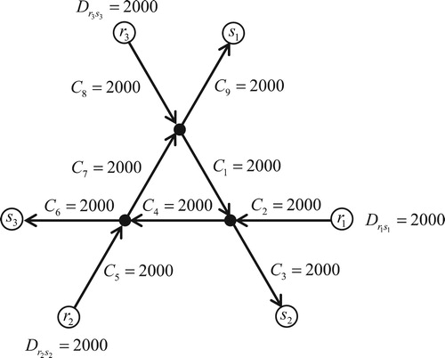
5.1. Scenario 1: multiple origin-destination pairs with a single route

The first example network of Bliemer et al. (2014) is shown in Figure 6. It possesses rotational symmetry. All links have a capacity of 2000 veh/h. There are three origin-destination pairs with one route each: to reach the destination, all traffic must traverse two-thirds of the inner triangle counter-clockwise. The demand for each origin–destination pair is 2000 veh/h. The time period of the simulation is 2 h. The Tampère et al. (2011) node model is used for the flow propagation.

Figure 6. Network with multiple origin-destination pairs with a single route (Bliemer et al. 2014, 377). Demands and capacities in veh/h.

Because this example has no route choice, the resulting flows on the network are exactly the same as reported by Bliemer et al. (2014). They can be computed in the exact same way. The only thing we do differently is the travel time calculation. Since Bliemer et al. (2014) use Equation (15) for link delays, the computation of route delays simplifies to Equation (11). Hence they report a route delay of (Bliemer et al. 2014, 378) (42) ${\tau }_{\mathrm{r}\mathrm{o}\mathrm{u}\mathrm{t}\mathrm{e}}^{\mathrm{q}\mathrm{u}\mathrm{e}\mathrm{u}\mathrm{e}}=\left(\frac{1}{{\alpha }_2{\alpha }_4{\alpha }_7{\alpha }_9}-1\right)\frac{T}{2}=\left(\frac{1}{0.618\cdot 0.618\cdot 0.618\cdot 1}-1\right)\frac{2\text{ h}}{2}=3.236\text{ h}\text{.}$(42) Conversely, our new formula from Equation (19) predicts the following route delay: (43) $\begin{array}{rl}{\tau }_{\mathrm{r}\mathrm{o}\mathrm{u}\mathrm{t}\mathrm{e}}^{\mathrm{q}\mathrm{u}\mathrm{e}\mathrm{u}\mathrm{e}}& ={\tau }_2^{\mathrm{q}\mathrm{u}\mathrm{e}\mathrm{u}\mathrm{e}}+{\tau }_4^{\mathrm{q}\mathrm{u}\mathrm{e}\mathrm{u}\mathrm{e}}+{\tau }_7^{\mathrm{q}\mathrm{u}\mathrm{e}\mathrm{u}\mathrm{e}}+{\tau }_9^{\mathrm{q}\mathrm{u}\mathrm{e}\mathrm{u}\mathrm{e}}\\ & =\frac{f_2}{q_2}\left(\frac{1}{{\alpha }_2}-1\right)\frac{T}{2}+\frac{f_4}{q_4}\left(\frac{1}{{\alpha }_4}-1\right)\frac{T}{2}+\frac{f_7}{q_7}\left(\frac{1}{{\alpha }_7}-1\right)\frac{T}{2}+\frac{f_9}{q_9}\left(\frac{1}{{\alpha }_9}-1\right)\frac{T}{2}\\ & =\frac{2000\text{ veh/h}}{2000\text{ veh/h}}\left(\frac{1}{0.618}-1\right)\frac{2\text{ h}}{2}+\frac{4000\text{ veh/h}}{2000\text{ veh/h}}\left(\frac{1}{0.618}-1\right)\frac{2\text{ h}}{2}+\frac{4000\text{ veh/h}}{2000\text{ veh/h}}\left(\frac{1}{0.618}-1\right)\frac{2\text{ h}}{2}\\ & +\frac{2000\text{ veh/h}}{472\text{ veh/h}}\left(\frac{1}{1}-1\right)\frac{2\text{ h}}{2}\\ & =0.618\text{ h}+1.236\text{ h}+1.236\text{ h}+0=3.090\text{ h}\text{.}\end{array}$(43)

As predicted in the Appendix, the delay we calculate is smaller than the delay calculated in Equation (42).

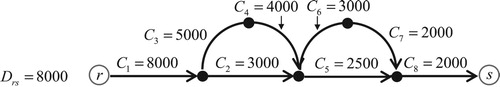
5.2. Scenario 2: single origin-destination pair with multiple routes

The second example network of Bliemer et al. (2014) is shown in Figure 7. All links have a free-flow travel time of 0.02 h. This example features route choice among four routes, with the multinomial logit model determining route choice probabilities (44) $\frac{e^{-\theta {\tau }_{\text{route}}}}{\sum _{\text{routes}}{e}^{-\theta {\tau }_{\text{route}}}}$(44) with $\theta =1{\text{h}}^{-1}$ and a total demand of 8000 veh/h for a 2 h time period. All nodes again use the Tampère et al. (2011) model. We solve the same flow propagation problem as Bliemer et al. (2014).

Figure 7. Network with a single origin-destination pair with multiple routes (Bliemer et al. 2014, 379). Demands and capacities in veh/h.

The equilibrium link flows, route demands and travel times are reported in Tables 2 and 3. As predicted in Section 4.1, drivers are less hesitant to choose routes with multiple bottlenecks, resulting in lower travel times for routes through link 2 and thus more drivers choosing them. This increases the queuing on link 1 and reducing the queue on link 4.

Table 2. Comparison of stochastic user-equilibrium link flows for Scenario 2.

Link $a$	Equilibrium inflow $q_a$		Equilibrium flow reduction factor ${\alpha }_a$
	Bliemer et al. (2014) result	Our result	Bliemer et al. (2014) result	Our result
1	8000 veh/h	8000 veh/h	0.845	0.822
2	3000 veh/h	3000 veh/h	0.655	0.655
3	3762 veh/h	3578 veh/h	1.000	1.000
4	3762 veh/h	3578 veh/h	0.696	0.732
5	2500 veh/h	2500 veh/h	0.444	0.444
6	2083 veh/h	2083 veh/h	0.960	0.960
7	2000 veh/h	2000 veh/h	0.444	0.444
8	2000 veh/h	2000 veh/h	1.000	1.000

Table 3. Comparison of stochastic user-equilibrium route demands and travel times for Scenario 2.

	Equilibrium demand		Equilibrium travel time
Route	Bliemer et al. (2014) result	Our result	Bliemer et al. (2014) result	Our result
1-2-5-8	1941 veh/h	1990 veh/h	3.146 h	3.120 h
1-2-6-7-8	1608 veh/h	1658 veh/h	3.334 h	3.302 h
1-3-4-5-8	2423 veh/h	2374 veh/h	2.924 h	2.944 h
1-3-4-6-7-8	2028 veh/h	1978 veh/h	3.102 h	3.126 h

The convergence of the equilibrium over the iterations is compared in Table 4. Despite that we use the same method of successive averages with the same weights $i^{-0.5}$, we typically reach the same level of convergence in about half the number of iterations. This is consistent with our prediction in Section 4.1.

Table 4. Comparison of stochastic user-equilibrium convergence speed for Scenario 2.

	Iteration number
Relative gap	Bliemer et al. (2014) result	Our result
< 10^−1	9	1
< 10^−2	13	11
< 10^−3	22	14
< 10^−4	33	16
< 10^−5	47	19
< 10^−6	63	29
< 10^−7	82	41
< 10^−8	> 100	56

5.3. Scenario 3: fixed routes with horizontal queuing and spillback

Finally, we revisit an example of Brederode et al. (2019, 15–19) which uses the same network as Figure 7.⁴ Instead of route choice, this example features horizontal queuing and spillback. We compare their results with our own modelling proposal from Section 4.3. Both methods start with a quasi-dynamic flow propagation calculation without spillback, which can be solved with Bliemer et al. (2014).

Then our methods diverge. Brederode et al. (2019) proceed with a DTA-like dynamic flow propagation with the previous results as initial conditions. The resulting cumulative inflow and outflow curves are used to compute flows and travel times with spillback.

In contrast, we repeatedly solve the same quasi-dynamic flow propagation problem with adjusted link inflow capacities $r_a$ to account for spillback within the time period $\left[0,T\right]$ (Raadsen and Bliemer 2018, 4): (45) $r_a=min\left({\alpha }_a{q}_a+\frac{L_a}{T}{K}_a^{\mathrm{q}\mathrm{u}\mathrm{e}\mathrm{u}\mathrm{e}}\left({\alpha }_a{q}_a\right),C_a^{\mathrm{in}}\right)$(45) where $C_a^{\mathrm{in}}$ indicates the link inflow capacity without spillback. Equation (45) means that the inflow is constrained by the outflow ${\alpha }_a{q}_a$ plus the number of vehicles it can store at the corresponding density $K_a^{\mathrm{q}\mathrm{u}\mathrm{e}\mathrm{u}\mathrm{e}}\left({\alpha }_a{q}_a\right)$. We refer to Raadsen and Bliemer (2018) for more information on this quasi-dynamic flow propagation technique. Afterwards, we use Equation (40) to produce travel times with spillback.

As before, all links are 2 km long and have a free speed of 100 km/h. The capacities are the same as in Figure 7. For all links, the speed in free-flow now depends on traffic conditions, with the speed at capacity being 80 km/h. The jam density on all links is 180 veh/km/lane. Links 5 and 7 have one lane. Link 1 has four lanes. All other links have two lanes. The fundamental diagram shapes are quadratic-linear (Smulders 1990, 117). The fixed route demands are listed in Table 5.

Table 5. Route demands for Scenario 3 (Brederode et al. 2019, 16).

Route	Demand
1-2-5-8	5867 veh/h
1-2-6-7-8	984 veh/h
1-3-4-5-8	984 veh/h
1-3-4-6-7-8	165 veh/h

The results are shown in Table 6. The final flows are similar despite the methodological differences in spillback modelling. Congestion spills back into the origin which we model as a vertical queue. Queue lengths and travel times for links are computed with Equations (38) and (40).

Table 6. Link flows, queue lengths, and travel times for Scenario 3.

Link $a$	Outflow ${\alpha }_a{q}_a$			Flow reduction factor ${\alpha }_a$		Our queue length $L_a^{\mathrm{q}\mathrm{u}\mathrm{e}\mathrm{u}\mathrm{e}}$		Our travel time ${\tau }_a$
	Result without spillback	Brederode et al. (2019) final result	Our final result	Result without spillback	Our final result	Result without spillback	Final result	Result without spillback	Final result
origin	8000 veh/h	n/a	2796 veh/h	1.000	0.349	n/a	n/a	0.000 h	1.862 h
1	3503 veh/h	2091 veh/h	2250 veh/h	0.438	0.805	10.03 km	2.86 km	1.183 h	0.685 h
2	2416 veh/h	1722 veh/h	1756 veh/h	0.805	0.911	13.30 km	3.56 km	0.411 h	0.329 h
3	503 veh/h	301 veh/h	323 veh/h	1.000	1.000	0.00 km	0.00 km	0.020 h	0.020 h
4	503 veh/h	302 veh/h	323 veh/h	1.000	1.000	0.00 km	0.00 km	0.020 h	0.020 h
5	1581 veh/h	1709 veh/h	1701 veh/h	0.632	0.956	29.31 km	3.85 km	1.252 h	0.157 h
6	419 veh/h	291 veh/h	299 veh/h	1.000	1.000	0.00 km	0.00 km	0.020 h	0.020 h
7	419 veh/h	291 veh/h	299 veh/h	1.000	1.000	0.00 km	0.00 km	0.021 h	0.021 h
8	2000 veh/h	2000 veh/h	2000 veh/h	1.000	1.000	0.00 km	0.00 km	0.025 h	0.025 h

The modelling of spillback improves the realism of our average queue lengths per link. As predicted in Section 4.3 queue lengths still exceed the 2 km link lengths because $f_a/q_a>2$. Spillback improves our travel times ${\tau }_a$ near the bottlenecks but deteriorates travel times upstream. Brederode et al. (2019, 17) show cumulative inflow and outflow curves for link 5 from their calculation. These correspond to an average travel time of 0.084 h, which can be compared to our final result of 0.157 h.

6. Conclusions

In this paper, we derived a new formula for link travel times in quasi-dynamic assignment, theoretically underpinned with vertical queuing and instantaneous propagation of traffic flows. We formulated requirements for both the absolute correctness and relative correctness of the travel times, and showed that the existing travel time computation procedures listed in Table 1 violate multiple. Contrary to this, we demonstrated that our own proposed definition of link travel times in Equation (19) does satisfy all requirements.

We also showed that our definition of link travel times has further advantages:

• the new travel time definition may speed up convergence of equilibrium traffic assignments;

• when used in a travel demand model, public transport travel times can be modelled consistently, including demand-responsive transport;

• pathfinding and fleet dispatching algorithms can be used directly with congested link travel times;

• using a fundamental diagram, the vertical queuing model can be transformed into the horizontal queuing model of Equation (40), to which the flow propagation model of Raadsen and Bliemer (2018) can contribute spillback and other interactions between bottlenecks;

• it is easy to introduce further extensions to account for stationary queues associated with traffic lights, to model traffic control optimised for the network flows, and to produce different travel times for different vehicle classes.

The practicality of our new link travel time formula was demonstrated with three example scenarios from literature. We look forward to uses of our new formula in larger practical studies and all sophisticated possibilities quasi-dynamic assignment has to offer.

Acknowledgement

This research effort was undertaken for the project Spatial and Transport impacts of Automated Driving (STAD), part of the research programme Smart Urban Regions of the Future (SURF) of the Netherlands Organisation for Scientific Research (NWO).

Disclosure statement

No potential conflict of interest was reported by the author(s).

ORCID

Jeroen P. T. van der Gun http://orcid.org/0000-0002-6522-3657

Adam J. Pel http://orcid.org/0000-0003-3754-5779

Bart van Arem http://orcid.org/0000-0001-8316-7794

Additional information

Funding

This work was supported by the Nederlandse Organisatie voor Wetenschappelijk Onderzoek.

Notes

1 An alternative solution is to instead get rid of instantaneous flow propagation, but then the quasi-dynamic model turns into a traditional dynamic model (with rectangular demand profiles and without spillback).

2 For simplicity, this example assumes fixed exit capacities, but they could also be variable, resulting from a node model.

3 Daganzo and Sheffi (1977, 260) recommend the gamma distribution only for short links and suggest the normal distribution otherwise, but the normal distribution may generate negative link costs hindering the Dijkstra algorithm.

4 Brederode et al. (2019) display the network mirrored vertically and with different link numbers.

Appendix

In this appendix we explore the derivation of the travel time formula in case we do not linearise cumulative inflow and outflow of each link as in Section 2.3, ignoring Requirement III.

The total delay $f_p{\tau }_p^{\mathrm{q}\mathrm{u}\mathrm{e}\mathrm{u}\mathrm{e}}$ on each link $p\in P_a$ equals the surface under its cumulative inflow curve minus the surface under its cumulative outflow curve. If we sum the cumulative inflow curves of all links $p\in P_a$ to construct the cumulative inflow curve of link $a$, the surface underneath is the sum of the surfaces under the separate cumulative inflow curves. Likewise, if we sum the cumulative outflow curves of all links $p\in P_a$ to construct the cumulative outflow curve of link $a$, the surface underneath is the sum of the surfaces under the separate cumulative outflow curves. Therefore, the total delay $f_a{\tau }_a^{\mathrm{q}\mathrm{u}\mathrm{e}\mathrm{u}\mathrm{e}}$ on link $a$, i.e. the surface under the combined cumulative inflow curve minus the surface under the combined cumulative outflow curve, that equals (A1) $f_a{\tau }_a^{\mathrm{q}\mathrm{u}\mathrm{e}\mathrm{u}\mathrm{e}}=\sum _{p\in P_a}{f}_p{\tau }_p^{\mathrm{q}\mathrm{u}\mathrm{e}\mathrm{u}\mathrm{e}}.$(A1) This clearly yields the same total travel time as Bliemer et al. (2014), but it is distributed differently so that all users of the same link experience the same travel time on that link. Rearranging and substituting Equation (10) for ${\tau }_p^{\mathrm{q}\mathrm{u}\mathrm{e}\mathrm{u}\mathrm{e}}$, we obtain (A2) ${\tau }_a^{\mathrm{q}\mathrm{u}\mathrm{e}\mathrm{u}\mathrm{e}}=\sum _{p\in P_a}\frac{f_p}{f_a}{\tau }_p^{\mathrm{q}\mathrm{u}\mathrm{e}\mathrm{u}\mathrm{e}}=\sum _{p\in P_a}\frac{f_p}{f_a}\frac{1}{\prod _{p^{\mathrm{\prime }}\in {\eta }_p}{\alpha }_{p^{\mathrm{\prime }}}}\left(\frac{1}{{\alpha }_a}-1\right)\frac{T}{2f_a}=\sum _{p\in P_a}\frac{f_p^2}{f_a{q}_p}\left(\frac{1}{{\alpha }_a}-1\right)\frac{T}{2}.$(A2) Compared to Equation (19), we now have a coefficient of ${\sum }_{p\in P_a}{f}_p^2/\left(f_a{q}_p\right)$ instead of $f_a/q_a$. In general, the delay calculated by Equation (A2) is larger than the delay calculated by Equation (19), because the weighted arithmetic mean of $1/{\prod }_{p^{\mathrm{\prime }}\in {\eta }_p}{\alpha }_{p^{\mathrm{\prime }}}$ is greater than or equal to the weighted harmonic mean of the same data with the same weights $f_p/f_a$: (A3) $\sum _{p\in P_a}\frac{f_p^2}{f_a{q}_p}=\sum _{p\in P_a}\frac{f_p}{f_a}\frac{1}{\prod _{p^{\mathrm{\prime }}\in {\eta }_p}{\alpha }_{p^{\mathrm{\prime }}}}\ge \frac{1}{\sum _{p\in P_a}\frac{f_p}{f_a}\prod _{p^{\mathrm{\prime }}\in {\eta }_p}{\alpha }_{p^{\mathrm{\prime }}}}=\frac{1}{\sum _{p\in P_a}\frac{q_p}{f_a}}=\frac{f_a}{q_a}.$(A3) For example, in Section 3.2, the demand-weighted average travel time on link 3 based on Equation (30) is (A4) $\frac{f_{\mathrm{AC},13}{\tau }_{\mathrm{AC},13,3}+f_{\mathrm{AC},23}{\tau }_{\mathrm{AC},23,3}}{f_3}=\frac{3000\text{veh/h}\cdot 35\text{min}+3000\text{veh/h}\cdot 65\text{min}}{6000\text{veh/h}}=50\text{min}\text{.}$(A4) This is indeed greater than the $45\text{min}$ resulting from Equation (36).

Aside from the theoretical problem with using Equation (A2) discussed in the main text, more reasons to avoid using it are revealed after combining with Equations (20) and (1): (A5) ${\tau }_a=\left\{\begin{array}{ll}{\tau }_a^{\mathrm{ff}}& \text{if }{q}_a\le C_a,\\ {\tau }_a^{\mathrm{ff}}+\sum _{p\in P_a}\frac{f_p^2}{f_a^2}\frac{q_a}{q_p}\left(\frac{f_a}{C_a}-\frac{f_a}{q_a}\right)\frac{T}{2}& \text{if }{q}_a\ge C_a.\end{array}\right.$(A5) Unlike Equation (21), derivatives with respect to $f_a$ and $q_a$ depend on which $f_p$ or $q_p$ is varied. Moreover, for $q_a\ge C_a$, we can write (A6) ${\tau }_a^{\mathrm{q}\mathrm{u}\mathrm{e}\mathrm{u}\mathrm{e}}=\sum _{p\in P_a}\frac{f_p^2}{f_a^2}\frac{q_a}{q_p}\left(\frac{f_a}{C_a}-\frac{f_a}{q_a}\right)\frac{T}{2}=\frac{\sum _{p\in P_a}\frac{f_p^2}{q_p}}{f_a}\left(\frac{q_a}{C_a}-1\right)\frac{T}{2}=\frac{\sum _{p\in P_a}\frac{f_p^2}{q_p}}{\sum _{p\in P_a}{f}_p}\left(\frac{q_a}{C_a}-1\right)\frac{T}{2},$(A6) so for any particular $p\in P_a$ we have (A7) $\mathrm{\forall }p\in P_a:{\tau }_a^{\mathrm{q}\mathrm{u}\mathrm{e}\mathrm{u}\mathrm{e}}=\frac{\frac{f_p^2}{q_p}+\sum _{p^{\mathrm{\prime }}\in P_a\mathrm{\setminus }\left\{p\right\}}\frac{f_{p^{\mathrm{\prime }}}^2}{q_{p^{\mathrm{\prime }}}}}{f_p+\sum _{p^{\mathrm{\prime }}\in P_a\mathrm{\setminus }\left\{p\right\}}{f}_{p^{\mathrm{\prime }}}}\left(\frac{q_a}{C_a}-1\right)\frac{T}{2},$(A7) whose derivative towards demand component $f_p$ follows from the quotient rule: (A8) $\begin{array}{rl}\mathrm{\forall }p\in P_a:\frac{\mathrm{\partial }{\tau }_a^{\mathrm{q}\mathrm{u}\mathrm{e}\mathrm{u}\mathrm{e}}}{\mathrm{\partial }{f}_p}& =\frac{\left(f_p+\sum _{p^{\mathrm{\prime }}\in P_a\mathrm{\setminus }\left\{p\right\}}{f}_{p^{\mathrm{\prime }}}\right)\left(2\frac{f_p}{q_p}\right)-\left(\frac{f_p^2}{q_p}+\sum _{p^{\mathrm{\prime }}\in P_a\mathrm{\setminus }\left\{p\right\}}\frac{f_{p^{\mathrm{\prime }}}^2}{q_{p^{\mathrm{\prime }}}}\right)}{{\left(f_p+\sum _{p^{\mathrm{\prime }}\in P_a\mathrm{\setminus }\left\{p\right\}}{f}_{p^{\mathrm{\prime }}}\right)}^2}\left(\frac{q_a}{C_a}-1\right)\frac{T}{2}\\ & =\frac{2\frac{f_p}{q_p}-\sum _{p^{\mathrm{\prime }}\in P_a}\frac{f_{p^{\mathrm{\prime }}}^2}{f_a{q}_{p^{\mathrm{\prime }}}}}{f_a}\left(\frac{q_a}{C_a}-1\right)\frac{T}{2}=\frac{2\frac{1}{\prod _{p^{\mathrm{\prime }}\in {\eta }_p}{\alpha }_{p^{\mathrm{\prime }}}}-\sum _{p^{\mathrm{\prime }}\in P_a}\frac{f_{p^{\mathrm{\prime }}}}{f_a}\frac{1}{\prod _{p^{\mathrm{\prime }\mathrm{\prime }}\in {\eta }_{p^{\mathrm{\prime }}}}{\alpha }_{p^{\mathrm{\prime }\mathrm{\prime }}}}}{f_a}\left(\frac{q_a}{C_a}-1\right)\frac{T}{2}.\end{array}$(A8) From this, we can see that the properties of Equation (23) no longer hold. For $q_a\in \left(C_a,f_a\right]$, instead of $\mathrm{\partial }{\tau }_a^{\mathrm{q}\mathrm{u}\mathrm{e}\mathrm{u}\mathrm{e}}/\mathrm{\partial }{f}_p>0$, we now have (A9) $\mathrm{\forall }p\in P_a:\mathrm{sgn}\frac{\mathrm{\partial }{\tau }_a^{\mathrm{q}\mathrm{u}\mathrm{e}\mathrm{u}\mathrm{e}}}{\mathrm{\partial }{f}_p}=\mathrm{sgn}\left(\frac{1}{\prod _{p^{\mathrm{\prime }}\in {\eta }_p}{\alpha }_{p^{\mathrm{\prime }}}}-\frac{1}{2}\sum _{p^{\mathrm{\prime }}\in P_a}\frac{f_{p^{\mathrm{\prime }}}}{f_a}\frac{1}{\prod _{p^{\mathrm{\prime }\mathrm{\prime }}\in {\eta }_{p^{\mathrm{\prime }}}}{\alpha }_{p^{\mathrm{\prime }\mathrm{\prime }}}}\right).$(A9) This implies that if:

• the exit capacity of the considered link is fixed;

• we increase a particular demand component $f_p$;

• due to some upstream bottleneck, this extra demand does not reach the considered link within the study period ($q_p$ constant);

• other demand components and flow components also remain the same;

• the severity $1/{\prod }_{p^{\mathrm{\prime }}\in {\eta }_p}{\alpha }_{p^{\mathrm{\prime }}}$ of the upstream bottlenecks of the demand component that increases is less than half the demand-weighted severity of upstream bottlenecks of the entire link demand;

then the increase in link demand leads to a decrease in link travel time, violating Requirement IV. Like the issues in Section 3.2, this is not possible in static assignment, dynamic assignment, or reality.

Because of the violation of both Requirements III and IV, we recommend to not use Equation (A2).

References

- Bakker, D., P. Mijjer, and F. Hofman. 1994. “QBLOK: een toedelingsmethodiek voor het modelleren van de afhankelijkheid tussen knelpunten en de voorspelling van blokkades.” In Colloquium Vervoersplanologisch Speurwerk 7994. Colloquium Vervoersplanologisch Speurwerk, edited by J. M. Jager, 313–332. Amsterdam.
- Bellman, R. 1958. “On a Routing Problem.” Quarterly of Applied Mathematics 16 (1): 87–90. doi: 10.1090/qam/102435
- Bifulco, G. N., and U. Crisalli. 1998. “Stochastic User Equilibrium and Link Capacity Constraints: Formulation and Theoretical Evidencies.” Proceedings of the European Transport Conference, Loughborough, UK, 85–96.
- Bliemer, M. C. J., M. P. H. Raadsen, E. Smits, B. Zhou, and M. G. H. Bell. 2014. “Quasi-Dynamic Traffic Assignment with Residual Point Queues Incorporating a First Order Node Model.” Transportation Research Part B 68: 363–384. doi: 10.1016/j.trb.2014.07.001
- Brederode, L., A. Pel, L. Wismans, E. De Romph, and S. Hoogendoorn. 2019. “Static Traffic Assignment with Queuing: Model Properties and Applications.” Transportmetrica A: Transport Science 15 (2): 179–214. doi: 10.1080/23249935.2018.1453561
- Bundschuh, M., P. Vortisch, and T. Van Vuuren. 2006. “Modelling Queues in Static Traffic Assignment.” European Transport Conference, Strasbourg, France.
- Bureau of Public Roads, ed. 1964. “Theory.” In Traffic Assignment Manual for Application with a Large, High Speed Computer, V1–V24. Washington, DC: U.S. Government Printing Office.
- Cascetta, E., A. Nuzzolo, F. Russo, and A. Vitetta. 1996. A Modified Logit Route Choice Model Overcoming Path Overlapping Problems. Specification and Some Calibration Results for Interurban Networks, 697–711. Oxford: Pergamon.
- Daganzo, C. F. 1995. “The Cell Transmission Model, Part II: Network Traffic.” Transportation Research Part B 29 (2): 79–93. doi: 10.1016/0191-2615(94)00022-R
- Daganzo, C. F., and Y. Sheffi. 1977. “On Stochastic Models of Traffic Assignment.” Transportation Science 11 (3): 253–274. doi: 10.1287/trsc.11.3.253
- Dijkstra, E. W. 1959. “A Note on Two Problems in Connexion with Graphs.” Numerische Mathematik 1 (1): 269–271. doi: 10.1007/BF01386390
- Ford, L. R. 1956. Network Flow Theory, P-923. Santa Monica, CA: RAND Corporation.
- Gentile, G. 2018. “New Formulations of the Stochastic User Equilibrium with Logit Route Choice as an Extension of the Deterministic Model.” Transportation Science 52 (6): 1297–1588. doi: 10.1287/trsc.2018.0839
- Gentile, G., P. Velonà, and G. E. Cantarella. 2014. “Uniqueness of Stochastic User Equilibrium with Asymmetric Volume-Delay Functions for Merging and Diversion.” EURO Journal on Transportation and Logistics 3 (3-4): 309–331. doi: 10.1007/s13676-013-0042-0
- Hart, P. E., N. J. Nilsson, and B. Raphael. 1968. “A Formal Basis for the Heuristic Determination of Minimum Cost Paths.” IEEE Transactions on Systems Science and Cybernetics 4 (2): 100–107. doi: 10.1109/TSSC.1968.300136
- Lam, W. H. K., and Y. Zhang. 2000. “Capacity-Constrained Traffic Assignment in Networks with Residual Queues.” Journal of Transportation Engineering 126 (2): 121–128. doi: 10.1061/(ASCE)0733-947X(2000)126:2(121)
- Lebacque, J. P., and M. M. Khoshyaran. 2005. “First-Order Macroscopic Traffic Flow Models: Intersection Modeling, Network Modeling.” In Transportation and Traffic Theory: Flow, Dynamics and Human Interaction - Proceedings of the 16th International Symposium on Transportation and Traffic Theory, edited by H. S. Mahmassani, 365–386. Oxford: Elsevier.
- Lighthill, M. J., and G. B. Whitham. 1955. “On Kinematic Waves II. A Theory of Traffic Flow on Long Crowded Roads.” Proceedings of the Royal Society of London A 229 (1178): 317–345.
- Nakayama, S., and R. Connors. 2014. “A Quasi-Dynamic Assignment Model That Guarantees Unique Network Equilibrium.” Transportmetrica A 10 (7): 669–692. doi: 10.1080/18128602.2012.751685
- Raadsen, M. P. H., and M. C. J. Bliemer. 2018. General Solution Scheme for the Static Link Transmission Model (ITLS-WP-18-21). Sydney: Institute of Transport and Logistics Studies.
- Raadsen, M. P. H., M. C. J. Bliemer, and M. G. H. Bell. 2016. “An Efficient and Exact Event-Based Algorithm for Solving Simplified First Order Dynamic Network Loading Problems in Continuous Time.” Transportation Research Part B 92 (B): 191–210. doi: 10.1016/j.trb.2015.08.004
- Richards, P. I. 1956. “Shock Waves on the Highway.” Operations Research 4 (1): 42–51. doi: 10.1287/opre.4.1.42
- Smulders, S. 1990. “Control of Freeway Traffic Flow by Variable Speed Signs.” Transportation Research Part B 24B (2): 111–132. doi: 10.1016/0191-2615(90)90023-R
- Tajtehranifard, H., A. Bhaskar, N. Nassir, M. M. Haque, and E. Chung. 2018. “A Path Marginal Cost Approximation Algorithm for System Optimal Quasi-Dynamic Traffic Assignment.” Transportation Research Part C 88: 91–106. doi: 10.1016/j.trc.2018.01.002
- Tampère, C. M. J., R. Corthout, D. Cattrysse, and L. H. Immers. 2011. “A Generic Class of First Order Node Models for Dynamic Macroscopic Simulation of Traffic Flows.” Transportation Research Part B 45 (1): 289–309. doi: 10.1016/j.trb.2010.06.004