Methods for Incorporating Measurement Error in Value-Added Models and Teacher Classifications

Abstract

The position statement on value-added models published by the American Statistical Association (ASA) suggested guidelines and issues to consider when using value-added models as a component of a teacher evaluation system. One suggestion offered is that value-added results should be accompanied by measures of precision. It is important, however, to go beyond simply reporting measures of precision alongside point estimates, but instead to formally include measures of precision into the value-added models and teacher classification systems. This practice will lead to improved inferences and reduced misclassification rates. Therefore, the aim of this article is to offer two suggested approaches for including measures of precision into the value-added model process. The first suggestion is to account for measurement error in student test scores and is motivated by the claim that measurement error is of little concern when the model conditions on at least three test scores. The second suggestion is to directly incorporate standard errors of the point estimates when forming overall classifications regarding teacher effects. This is intended to demonstrate ways in which teacher misclassification rates can be minimized.

KEY WORDS::

• Accountability
• Error-In-Variables
• Precision

1. INTRODUCTION

The American Statistical Association (ASA) recently published a position statement on value-added models (VAM) in which suggestions and cautions are offered in an attempt to improve the inferences drawn from VAMs (ASA 2014). The ASA position article offers an important platform by which researchers and practitioners in the VAM community can more formally extend the ideas discussed in the statement via specific methodological approaches or experiences gathered from empirical results in applied settings.

In this spirit, I choose one issue noted in the ASA statement, precision. My intention is to extend the following statement in the ASA position article, “Estimates from VAMs should always be accompanied by measures of precision and a discussion of the assumptions and possible limitations of the model” by offering two proposals on how measures of precision might be incorporated into the modeling and decision-making process. In what follows I argue that two sources of uncertainty—measurement error in student test scores and imprecision associated with teacher-level scores—need to be recognized and appropriately integrated into the general value-added model process.

The ideas in this article are motivated by two issues that have become somewhat common in the practice of VAM. First, I dissect the claim made by Sanders (2006) that measurement error in the student test scores is of little concern when the regression model conditions on at least three prior test scores. Second, VAM results are commonly used as a component in the overall teacher evaluation system. However, there tends to be an overreliance on point estimates to classify teachers, resulting in teacher classifications that seemingly fluctuate over time.

To address the former concern, I examine the claim analytically and demonstrate that the conditions necessary to support this claim are most likely implausible in real world scenarios. I then articulate an estimator that can be used to incorporate student-level measurement error into the model estimation. To address the latter concern, options for teacher classification are proposed that make use of the uncertainty in the estimate.

2 THE PRECISION OF STUDENT-LEVEL TEST SCORES

Observed test scores are the typical ingredients in a VAM, though it is known that regression models making use of these scores yield biased estimates of the model coefficients given that they are imperfect measures of a student’s true score (Greene 2000; Hausman 2001). However, Sanders (2006) suggested that the bias is eliminated to the point where it is “no longer of concern” (p. 5) when at least three predictors are used as covariates in the model. This argument appeals to a similar “bias compression” concept articulated by Lockwood and McCaffrey (2007) who showed that bias related to nonrandom sorting of students to classes decreases, under certain circumstances, as more prior score observations become available. We can explore the claim regarding measurement error analytically.

Test theory (Lord 1980) establishes the following relationship between a true score and an observed score, X = X* + U, where X is a matrix of observed scores, X* is a matrix of true (unobserved) scores, and U is a disturbance matrix with the same dimensions as X*. A true score regression can be written as (1) where y is an n × 1 vector of outcome scores, X* is an n × p model matrix containing p − 1 true prior test scores, β are the fixed effects, and . On substitution (2)

The assumptions used throughout the remainder of this discussion include U⊥X*, e⊥X*, and U⊥e. The elements of the disturbance matrix, U, are u_ij for the ith student on the jth test, , and is taken as the conditional standard error of measurement. Errors of measurement on different variables are assumed when j ≠ j′. From the preceding assumption on the N × J matrix U, we see that

2.1 Inconsistent Estimation of Model Parameters

From the set of previously proposed assumptions, we examine the behavior of a least-square estimate when observed scores are used in the model. First, we observe that cov(X, e*) ≠ 0: (3)

Equation (3(3) ) demonstrates the source of inconsistency in the ordinary least-square (OLS) estimate in general. But, we need to examine the behavior of the model with respect to measurement error more carefully as more predictors are added. Suppose we expand the model to view this through the lens of estimating a teacher effect such that X* = [X₁*, Z] and β′ = [β′, θ′] giving (4) where the matrix X₁* is n × p holding prior scores and a vector of 1’s corresponding to an intercept, and Z is an n × q indicator matrix linking student i to teacher k. In this case, the kth teacher effect is equivalent to the following given estimates for the prior test score coefficients (5)

Equation (5(5) ) can be used to illustrate the conditions under which the effect of the measurement error bias could be mitigated. Because Equation (5(5) ) is key, a full proof of its derivation from Equation (4(4) ) is provided in Appendix A.

If the variance of the term in Equation (5(5) ) were to approach 0 with increasing P, then the effect of the measurement error bias would become smaller with additional tests added as predictors. From the assumptions regarding the disturbance term, the variance of the product of these two random variables will be approximately .

Given that σ²_j > 0, we must require that for the variance term to approach 0. If the data-generating model for the test scores at time t for student i on test j contained in the matrix X₁* can be characterized as x_tij = x*_ij + u_tij, then and the individual coefficients added to the regression decrease at a rate that is approximately proportional to , where is the expected value of the coefficient when the model includes only one prior score. For instance, in a model with two predictors, and both would be about 1/2 the size of if it were in the model alone given that each score carries with it the same information regarding a student’s true ability.

Under these assumptions, will eventually sum to 0 with increasing P, though it is likely to require many more than three prior tests. However, this rests on the assumption that x*_ij is fixed over time and that is difficult to justify. In practice, we expect a student’s true state to change as they learn over time. In fact, if we do assume that the true score is fixed, then each new observed score is a different measure of the same latent trait and growth is simply a different random draw on the error term, u_tij.

2.1.1 Simulation Example

A brief simulation using 1000 replicates is provided to illustrate the preceding theory. The R code (R Core Team 2013) provided in the appendix can be used to replicate the simulation. The simulation generates 1000 students each with five observed scores and an outcome where the data-generating process for each observed score is x_tij = x*_ij + u_tij. Model coefficients are estimated using OLS via the lm function in R. Each model layers in one new observed score such that model 1 includes only one prior score, model 2 includes two scores, etc. The expected values of the coefficients are the means of the coefficients over all 1000 replicates.

Table 1. Expected values of model coefficients

Model
Model 1	0.91					0.82
Model 2	0.46	0.48				0.45
Model 3	0.31	0.33	0.33			0.31
Model 4	0.23	0.25	0.26	0.23		0.24
Model 5	0.18	0.20	0.21	0.18	0.20	0.19

The results in Table 1 show that the expected values of the model coefficients decrease at the rate approximately proportional to . The term decreases with more prior scores, but does not approach 0 with even five prior scores.

2.2 An Error-in-Variables Estimator

In contrast, if the underlying model generating observed scores is x_tij = x*_tij + u_tij, and if we expect x*_tij > x*_{t − 1, ij}, then it is not feasible to arrive at conditions supporting the idea that with increasing P; hence the inconsistency in the OLS estimate from Equation (3(3) ) remains. Therefore, it is important to have an estimator that can account for the measurement error, which can be arrived at simply: (6)

Taking the expectation over the measurement error distribution and treating the true score matrix as fixed, and . We arrive at these given the following, given that X* ⊥ U and U ⊥ y. Taking the observed scores in X gives (7)

Given an available estimate for , which we can take as the diagonal matrix S, with the cautions noted by Lockwood and McCaffrey (2014), it is simple to incorporate the uncertainty associated with the test scores into the model building process. Extending this to the mixed model is also straightforward as demonstrated by multiple authors (Goldstein 1995; AIR 2013; Lockwood and McCaffrey 2014).

The preceding shows that assuming measurement error bias is “no longer of concern” when the model conditions on three prior scores cannot be supported with a finite number of tests measuring a trait that is expected to change over time. As such, this leads to a different recommendation for model building: any model proposed for use in teacher evaluation systems must incorporate student-level measurement error into model estimation to properly yield unbiased estimates.

3 INCORPORATING UNCERTAINTY INTO TEACHER CLASSIFICATIONS

VAMs produce point estimates, such as medians or means of growth percentiles, empirical Bayes, or fixed effects, to indicate the impact on student achievement. These point estimates are often the basis for ranking teachers using a simple classification scheme. For example, it is common to find teacher VAM scores put into performance bins (e.g., quintiles) based on the point estimates (Loeb and Candelaria 2013) or for teachers with VAM scores in the lowest decile to be flagged for improvement.

The practice of assignment to performance bins using only observed scores increases the probability of misclassification and over time it degrades the credibility of the VAM results as teachers seemingly move across performance categories over time. In the end, this yields very little credibility to an accountability system when high-performing teachers appear as lower-performing teachers in subsequent years and vice-versa.

The ASA position statement suggests that “Estimates from VAMs should always be accompanied by measures of precision.” To build upon this statement with concrete recommendations, I propose options to consider that may be used to form classifications. Before doing so, it is important to understand that ignoring the measurement error in test scores may overstate the precision of the teacher VAM estimates.

For purposes of illustration, data from a large statewide test including 163,401 students, 4614 teachers, and 1147 schools are modeled. A test score in grade g is modeled as a function of two prior test scores obtained grades g − 1 and g − 2 as well as teacher and school random effects. In the first instance, the error in the predictor variables is ignored and in the second model the error in the student-achievement estimates is incorporated using an error-in-variables regression (Goldstein 1995).

The following statistic is then used to express the general instability of the teacher VAM scores (8) where is the mean (conditional) variance of the teacher effects and σ²_θ is the model-based (marginal) variance between teachers. This simply expresses the typical standard error as a fraction of the standard deviation between teachers. In the model that ignores measurement error in the predictors, we obtain a value of p = 0.66 and in the model that incorporates measurement error into the regression we observe p = 0.71. This shows that the precision of the teacher effects tends to be overstated when measurement error in the predictor variables is ignored.

3.1 Options for Classification

Given the VAM results, one could simply use the point estimates to place teachers into bins and then report the standard error of the teacher effect alongside the classification results. However, this classification method does not incorporate the uncertainty into the classification. In this section, I briefly provide four different ways in which the uncertainty in the estimate might be used when forming or reporting teacher VAM scores.

3.1.1 Method 1: Classification with Confidence Intervals

To illustrate the first approach, suppose it is required that teachers are assigned to one of four ordered performance bins. We could begin with assignment to a default category, say 3, and then form confidence intervals around the point estimate, , and bin the VAM scores based on the following rules:

This approach has been used in one state where we have implemented VAMs and formed teacher classifications. We found that the observed correlation between the teacher effects over time was 0.46, but 68% of teachers remained in the same performance bin from 1 year to the next when the uncertainty in the estimate was used to form the classifications. Additionally, large swings in the extremes (i.e., teachers changing from the lowest to highest performance bins and vice versa) was less than 0.1% (AIR 2013).

The approach is conservative with respect to teacher classification and has trade-offs worth considering with stakeholder groups involved in the accountability process. First, under the specific example provided teachers with the following condition and are tacitly assumed to fall into bin 3, even if the majority of their score distribution falls into the level 2 category. Additionally, teachers are only placed into bins 1 and 4 under highly stringent conditions. As such, this proposed approach will push larger proportions of teachers into the middle categories and make it somewhat more challenging to identify outlier teachers.

3.1.2 Method 2: Classification With Threshold

He, Selck, and Normand (2014) provided an exposition on methods for classifying hospitals on the basis of a performance measure. This line of work draws many parallels to the challenges also observed in teacher classification and provides comparisons between various classification approaches. In many respects, the policy context and motivation to classify teachers shares many similarities with the aims to classify hospitals. For example, in some policy circles, an ideal outcome for VAM is to support the identification of a “high tier” of teachers, or conversely a “lower tier,” where high-performing teachers may be eligible for rewards and low-performing teachers may be subject to sanctions. Hence, this approach can be adopted for use when forming teacher classifications based upon VAMs.

He, Selck, and Normand (2014) identified an optimal method for classification referred to as “PROB II.” This approach considers the posterior probability that the teacher effect exceeds a known threshold. An alternative method is provided and is shown to provide virtually identical results to PROB II with respect to misclassification referred to as the “SHR” or shrinkage method. This approach classifies teacher k into the 100(1 − c)% when exceeds a threshold, such as λ + σ_θΦ^{− 1}(c), where c identifies the estimates for teachers in the 100(1 − c)% tier. For instance, if the aim is to identify the top 10%, then the following condition is evaluated, . Given the similarity between the approaches proposed, I illustrate the SHR method, though further work is needed to examine PROB II.

One issue to consider is the optimal value for c that yields misclassification rates at an acceptable level. Here, I briefly explore via a simulation various options for the value of c. From the simulation it is possible to judge the sensitivity—the probability of assigning a true high tier teacher into the top tier, given that simulating data yield both a known true value and an estimate for each of the k teacher VAM scores.

For illustration, I generate data from a simple random effects model with two noisy measures as predictors each with reliability of about 0.9, y_imk = μ + ∑²_{j = 1}β_jx_ij + θ_k + θ_m + e_imk, where , , and , and true values for the fixed effects, μ, β₁, β₂ are set to 10, 1, and 0.5, respectively. The random effects are intended to mirror separable teacher and school effects such that the teacher value-added score is θ_k. The simulated data include 10,000 students nested in 400 teachers in 100 schools. Ten percent of the students are randomly dropped at each replicate to create an unbalanced design.

I run 500 replicates and within each replicate identify the number of observed values that exceed the criterion . The parameter c is a vector ranging from 0.5 to 0.9 in increments of 0.01, but the parameter λ is fixed at 0. Let P(c)_l denote the proportion of observed VAM scores above the threshold that are correctly classified given the true value of the VAM score, c ∈ {0.5, 0.51, …, 0.9} at replicate l.

Figure 1. Sensitivity using different values for the threshold parameter.

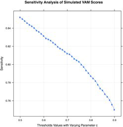
Figure 1 plots the mean sensitivity (i.e., mean of P(c)_l over all replicates) at the different values of the threshold. Similar to He, Selck, and Normand (2014), the sensitivity rates decline with higher values of c given it is somewhat more difficult to distinguish high performers in the tails. Because choosing a value for c is a policy-driven exercise, the sensitivity rates in Figure 1 can be used as a guide to consider values for that parameter. Those considering such an approach for classification might find it useful to simulate data using generating values that more closely resemble their jurisdictions as the data generated here are simply to illustrate the concept and are not designed to match values from a state testing program.

3.1.3 Method 3: Classification With Marginal Probability

Suppose assignment to multiple performance categories is required, but users are interested in the marginal probability that the teacher effect exceeds the cut for bin λ_j. We could simply report the classification and provide the probability that the effect exceeds the cut or classify the teacher only if the marginal probability exceeds a threshold using: (9)

This approach can be easily implemented and used to consider the mass of the teacher effect distribution over the range of classification categories.

3.1.4 Method 4: Classification With Conditional Probability

One other probability that may serve as a useful indicator is the conditional probability that , is above λ_j given that θ*_k is below the cut, . This statistic can be used to judge the risk of misclassification to a performance bin for individual teachers.

4 SUMMARY

My attempt in this article is to build upon the ASA’s general statements about precision, offering evidence for why it is important to incorporate uncertainty into model estimation and suggestions for how this might be done. The argument that measurement error in the predictors is of little concern when the model conditions on at least three prior test scores seems to be limited to a very myopic condition requiring assumptions that are unlikely to be true in real world scenarios. As a result, it is more important to have in hand estimators, such as an error-in-variables regression, that can directly incorporate test measurement error into the estimation process.

Additionally, teacher classification methods should also find ways in which the precision of the estimate should be incorporated into the classification method. If teacher classification is based on point estimates alone and standard errors of the point estimate are simply reported alongside the estimate, teacher classification ratings will vary over time in ways that seem implausible to users of the data. In student achievement testing, it is possible to design tests to maximize the amount of information near important cuts, such as the “proficient” cut score. Hence, it is feasible to control some of the variability in student scores near important cuts via design of the test. In contrast, this cannot be accomplished with VAM. Class assignment mechanisms at the beginning of a school year cannot be organized in ways that intentionally minimize error variance in an outcome collected after a year of instruction with a teacher.

One option that deserves future attention is ways in which teacher classification might resemble methods used in setting performance standards on student achievement tests, such as the bookmark method (Cizek 2001). In achievement testing, these methods connect items on a test to knowledge and skills students are expected to know and demonstrate with respect to the enacted curriculum. For instance, when a student is classified as proficient on the test, it implies something about what the students demonstrated with respect to the content, not how the student relates to other students in the population.

The challenge in projecting this concept to VAM is that it requires an external criterion allowing VAM point estimates to be ordered and related to other evaluation criterion. For example, suppose it is feasible to order the VAM point estimates by teacher and then have expert evaluators connect each point estimate along the continuum to another set of performance skills. If such an approach could be properly conceptualized and implemented, it may be possible to remove the normative nature of VAM classifications and move toward a criterion-related classification scheme.

APPENDIX A: PROOF DERIVING EQUATION 5 FROM EQUATION 4 AS A PARTITIONED REGRESSION

The normal equation for a partitioned regression is (McCulloch and Searle 2001) (A.1)

We can solve for θ as (A.2)

The matrix Z consists of q total columns with each column linking student i to the kth teacher. If we assume all students are nested in one and only one classroom, then (A.3) with inverse (A.4) where N_k is the column sum of the kth column in Z. If Z is a binary matrix linking student i to teacher k, the column sum is the number of students linked to the kth teacher.

The simple diagonal structure of Z′Z permits for the following solution for the kth column in Z, denoted as z_k. Because z_k has dimensions n × 1, its transpose remains conformable with X* and y, which have dimensions n × p and n × 1, respectively. Hence, Equation (A.2(A.2) ) can be reduced to the following to allow for a teacher-by-teacher solution: (A.5)

Solving for θ_k, assuming x_ij = x*_ij + u_ij in the final step, and assuming the model matrix X* includes a vector of 1’s corresponding to an intercept provides (A.6)

APPENDIX B

############################################## ###########################################

# R code to implement simulation described in section 1

%########################################## ############################################# ############################################ ##############

#  Generate data

 

N <- 1000 # Number of individuals

K <- 1000 # Number of replicates

 

### Matrices to store model coefficients

fm1_params <- matrix(0, nrow = K, ncol = 1)

fm2_params <- matrix(0, nrow = K, ncol = 2)

fm3_params <- matrix(0, nrow = K, ncol = 3)

fm4_params <- matrix(0, nrow = K, ncol = 4)

fm5_params <- matrix(0, nrow = K, ncol = 5)

 

true <- rnorm(N)

 

for(i in 1:K){

 

e1 <- rnorm(N, sd = .3)

e2 <- rnorm(N, sd = .3)

e3 <- rnorm(N, sd = .3)

e4 <- rnorm(N, sd = .3)

e5 <- rnorm(N, sd = .3)

 

x1 <- true + e1

x2 <- true + e2

x3 <- true + e3

x4 <- true + e4

x5 <- true + e5

 

y <- true + rnorm(N, sd = .3)

 

fm1 <- lm(y ∼ x1)

fm2 <- lm(y ∼ x1 + x2)

fm3 <- lm(y ∼ x1 + x2 + x3)

fm4 <- lm(y ∼ x1 + x2 + x3 + x4)

fm5 <- lm(y ∼ x1 + x2 + x3 + x4 + x5)

 

 

fm1_params[i, ] <- coef(fm1)[2]

fm2_params[i, ] <- coef(fm2)[2:3]

fm3_params[i, ] <- coef(fm3)[2:4]

fm4_params[i, ] <- coef(fm4)[2:5]

fm5_params[i, ] <- coef(fm5)[2:6]

 

cat(`Iteration', i, `\n')

 

}

 

### Compute expected values as means

colMeans(fm1_params)

colMeans(fm2_params)

colMeans(fm3_params)

colMeans(fm4_params)

colMeans(fm5_params)

 

### Expected sum of squared coefficients

sum(colMeans(fm1_params)^2)

sum(colMeans(fm2_params)^2)

sum(colMeans(fm3_params)^2)

sum(colMeans(fm4_params)^2)

sum(colMeans(fm5_params)^2)

References

- (2013), 2012 to 2013 Growth Model for Educator Evaluation Technical Report, Technical Report, AIR, Washington, DC. Available at http://www.engageny.org/sites/default/files/resource/attachments/2012-13-technical-report-for-grow-th-measures.pdf.
- (2014), ASA Statement on Using Value-Added Models for Educational Assessment, available at https://www.amstat.org/policy/pdfs/ASA_VAM_Statement.pdf.
- Cizek, G. J. (ed.) (2001), Setting Performance Standards: Concepts, Methods, and Perspectives, Mahwah, NJ: Lawrence Erlbaum Associates.
- Goldstein, H. (1995), Multilevel Statistical Models, London: Oxford University Press.
- Greene, W.H. (2000), Econometric Analysis (4th ed.), Saddle River, NJ: Prentice Hall.
- Hausman, J. (2001), Mismeasured Variables in Econometric Analysis: Problems From the Right and Problems From the Left, The Journal of Economic Perspectives, 15, 57–67.
- He, Y., Selck, F., and Normand, S.- L. T. (2014), On the Accuracy of Classifying Hospitals on Their Performance Measures, Statistics in Medicine, 33, 1081–1103.
- Lockwood, J., and McCaffrey, D.F. (2007), Controlling for Individual Heterogeneity in Longitudinal Models, With Applications to Student Achievement, Electronic Journal of Statistics 1, 223–252. Available at. http://dx.doi.org/10.1214/07-EJS057.
- ——— (2014), Correcting for Test Score Measurement Error in Ancova Models for Estimating Treatment Effects, Journal of Educational and Behavioral Statistics, 39, 22–52.
- Loeb, S., Candelaria, C.A. (2013), How Stable are Value-Added Estimates Across Years, Subjects, and Student Hroups? Technical Report, Carnegie Knowledge Network. Available at. http://www.carnegieknowledgenetwork.org/briefs/value-added/value-added-stability/.
- Lord, F.M. (1980), Applications of Item Response Theory to Practical Testing Problems, Hillsdale, NJ: Erlbaum.
- McCulloch, C.E., and Searle, S.R. (2001), Generalized, Linear, and Mixed Models, New York: Wiley.
- R Core Team (2013), “R: A Language and Environment for Statistical Computing” Computer software manual, Vienna, Austria: R Core Team. . Available at. http://www.R-project.org/
- Sanders, W.L. (2006), Comparisons Among Various Educational Assessment Value-Added Models. Available at. http://www.sas.com/resources/asset/vaconferencepaper.pdf.