Alternative Statistical Frameworks for Student Growth Percentile Estimation

Abstract

This article suggests two alternative statistical approaches for estimating student growth percentiles (SGP). The first is to estimate percentile ranks of current test scores conditional on past test scores directly, by modeling the conditional cumulative distribution functions, rather than indirectly through quantile regressions. This would remove the need for post hoc procedures required to ensure monotonicity of the estimated quantile functions, and for inversion of those functions to obtain SGP. We provide a brief empirical example demonstrating this approach and its potential benefits for handling discreteness of the observed test scores. The second suggestion is to estimate SGP directly from longitudinal item-level data, using multidimensional item response theory models, rather than from test scale scores. This leads to an isomorphism between using item-level data from one test to make inferences about latent student achievement, and using item-level data from multiple tests administered over time to make inferences about latent SGP. This framework can be used to solve the bias problems for current SGP methods caused by measurement error in both the current and past test scores, and provides straightforward assessments of uncertainty in SGP. We note practical problems that need to be addressed to implement our suggestions.

• Conditional distribution function
• Deconvolution
• Measurement error
• Multidimensional item response theory
• Teacher value-added.

INTRODUCTION

Student growth percentiles (SGP; Betebenner 2008, 2009, 2011; Castellano and Ho 2013) are currently being considered or used in more than half of the states in the country to gauge the academic progress of both individual students and groups of students. The widespread interest in SGP is in part due to their conceptual simplicity: each student’s current test score is expressed as a percentile rank in the distribution of current test scores among students who had the same past test scores. For example, an SGP of 70 for a student conveys that the student scored higher on the current test than 70% of his or her peers who had scored similarly in the past. SGP are commonly interpreted as a measure of relative growth or conditional status in achievement (Castellano and Ho 2013), and they do not require vertically scaled scores (Betebenner 2009) or assume that the test score scales have interval properties (Briggs and Betebenner 2009). Another appealing aspect of SGP is that they provide a student-level statistic that can be aggregated to higher levels (e.g., teachers or schools) to provide summaries of performance of groups of students sharing educational experiences. Typically, either the median or mean SGP is used as the group-level measure, and we use “MGP” to refer to either the mean or the median SGP of a group of students (Betebenner 2008; Castellano and Ho 2014). The MGP are interpreted by some stakeholders as measures of relative performance of different educational units and are being used as part of teacher and/or leader evaluations (e.g., Colorado Department of Education 2013; Georgia Department of Education 2014).

The articles by Guarino et al. (2014) and Walsh and Isenberg (2014) in this issue both provide valuable information about how MGP and teacher value-added measures differ. Walsh and Isenberg (2014) summarized existing literature on the comparison of the measures, and compared the two methods in a real teacher evaluation context in Washington, DC. They found that the two methods provide systematically different performance measures for teachers teaching students with different background characteristics, but which measure favors certain teachers depends on the choice of background characteristics examined. Guarino et al. used simulation to demonstrate that MGP are less able to recover true teacher impacts on student achievement than certain value-added methods, and presumably the differences between the estimators are correlated with the characteristics of the students in the simulated classrooms. They also demonstrated evidence that the circumstances required to cause the two types of measures to have systematic differences may exist in real data. Both articles note that the relative behavior of the measures may be influenced by the extent to which differentially effective teachers systematically teach different types of students, and that MGP will generally provide biased estimates of educator performance when teachers of different effectiveness systematically teach students of different prior achievement levels.

Both articles answer questions about the relative behavior of the performance measures using SGP as currently implemented in the freely available R (R Development Core Team 2013) package “SGP” (Betebenner et al. 2014), and we refer to that method as the “standard SGP approach.” An equally important question is whether the standard SGP approach is the optimal way to estimate the percentile rank of a student’s performance among peers with a similar achievement history. Researchers and policymakers studying and using SGP and MGP measures have tended to take the statistical procedures used by the standard SGP approach at face value. We argue here that some alternative frameworks for estimating SGP are possible and might be advantageous.

Our first suggestion is to estimate percentile ranks of current test scores conditional on past test scores directly, by modeling the conditional cumulative distribution functions (CDFs), rather than indirectly through quantile regressions. This would remove the need for procedures required to ensure monotonicity of the estimated quantile functions and for inversion of those functions to obtain SGP. Both of these aspects of the standard SGP approach make it difficult to determine properties of SGP estimators such as standard errors, whereas directly modeling the conditional CDFs moves the estimation into a well-studied statistical framework where estimators with known properties are available and where the discreteness of the observed test scores can be addressed more easily.

Our second suggestion is to estimate SGP directly from longitudinal item-level data, using multidimensional item response theory (MIRT) models (Haberman, von Davier, and Lee 2008; Reckase 2009), rather than from scale scores. This leads to an isomorphism between using item-level data from one test to make inferences about latent student achievement, and using item-level data from multiple tests administered over time to make inferences about latent SGP. This framework defines SGP in terms of latent achievement traits and their distributions in the target population, in contrast to defining SGP in terms of observed test scores and their distributions. If the MIRT model is appropriate for the data, this framework can be used to solve the bias problems for SGP caused by measurement error in both the current and past test scores, which has proven to be difficult to solve for the standard SGP approach. It also provides several candidate estimators for the latent SGP, which have corresponding estimates of variability, leading to straightforward assessments of uncertainty in SGP.

We discuss these suggestions in turn in the following sections. For each, we first discuss potential issues that may arise with the standard SGP approach, and suggest alternatives that may address these issues. We note some additional issues that these alternatives may introduce. We provide an empirical illustration of one of our suggestions but leave simulation studies and deeper empirical applications of our suggestions as future work given that our interest here is to open the discussion about alternative approaches to estimating SGP. We conclude with a brief discussion regarding limitations of SGP that exist regardless of how they are estimated.

2. ESTIMATION BY DIRECTLY MODELING CONDITIONAL CDFs

Because we will later be discussing issues with test score measurement error, we follow the notation of Carroll et al. (2006) by using W₁ to denote the observed current test score and W₀ to denote the observed prior test score. For clarity, we focus on the case where there is only a single prior test score, although both of our suggestions can be implemented when multiple past test scores are included in the conditioning. To simplify notation, we also do not use subscripts for individual students.

We first consider a simplified case in which observed test scores are modeled as continuous random variables, and later discuss the case where the discreteness of observed test scores is taken into account. In the continuous case, the SGP based on observed test scores is defined as (2) $$\rho (W_0,W_1):=F_{W_1|W_0}\left(W_1\right|W_0)={\int }_{-\infty }^{W_1}{p}_{W_1|W_0}\left(u\right|W_0)du,$$(2) where $p_{W_1|W_0}$ is the conditional density of W₁ given W₀ and $F_{W_1|W_0}$ is the corresponding conditional CDF. These distributions and the resulting SGP are defined with respect to some target population of students, such as all students tested at a given grade level in a state. The practical challenge is that the distributions are unknown and must be estimated from the longitudinal student-level data. We ignore the distinction between defining the SGP in terms of discrete percentile ranks, reported on a 0–100 scale, and the conditional CDF.

2.1 Potential Issues With the Standard Approach

Although $F_{W_1|W_0}\left(W_1\right|W_0)$ is the estimand of interest for SGP, the standard approach estimates it indirectly. Rather than modeling $F_{W_1|W_0}\left(W_1\right|W_0)$, it models the conditional quantile functions $F_{W_1|W_0}^{-1}\left(\tau \right|W_0)$ for selected percentile points τ, typically from 0.005 to 0.995 in increments of 0.01 (Betebenner et al. 2014). This introduces two related complications. The first is that while the true quantile functions must satisfy $F_{W_1|W_0}^{-1}\left(\tau \right|W_0)\le F_{W_1|W_0}^{-1}\left({\tau }^{*}\right|W_0)$ for τ ⩽ τ*, the estimated quantile functions will not generally satisfy these monotonicity constraints. The quantile function for each τ is estimated separately using quantile regression (Koenker 2005) parameterized using B-splines to provide flexibility in the conditional distributions (Betebenner 2009). The estimated functions are then manipulated post hoc to enforce the monotonicity constraints.¹

The second related complication introduced by the indirect estimation of $F_{W_1|W_0}\left(W_1\right|W_0)$ through quantile functions is that calculating the SGP for each student requires manually inverting the estimated quantile functions. Specifically, the SGP for a student is calculated by identifying the maximum predicted conditional quantile the current score is strictly greater than, rounding the corresponding percentile point up (to the hundredths place), and multiplying by 100. For instance, if a student’s current score lies between the τ = 0.595 and τ = 0.605 predicted quantiles, 0.595 is the maximum percentile point the student’s score is strictly greater than, making this student’s SGP 0.60 × 100 = 60 (Betebenner et al. 2014). This is a discontinuous function of the current score for each W₀.

Both of these complications make it difficult to evaluate properties of the SGP estimators from the standard approach. The approach estimates separate flexible quantile regressions for each percentile point, manipulates the estimated functions post hoc to ensure monotonicity, and then calculates the SGP as a discontinuous function of the estimated quantiles. The SGP estimator is thus defined implicitly by an algorithm rather than explicitly by a statistical model. This makes it difficult to assess to what extent SGP estimators are unbiased and what their sampling error might be so that standard errors can be estimated. The algorithmic approach to SGP calculations also makes it virtually impossible to implement corrections to SGP estimators for test score measurement error other than simulation-extrapolation (SIMEX; Cook and Stefanksi 1994; Carroll et al. 2006), in which additional measurement error is added to data to establish a functional relationship between the measurement error variance and a parameter estimate. This relationship is then projected backward to produce a parameter estimate intended to reflect what the estimate would have been had the data contained no measurement error. The potential value of SIMEX in the context of SGP is investigated by Shang (2012) and Shang, Van Iwaarden, and Betebenner (2014).

2.2 Potential Improvements

Because the conditional CDF $F_{W_1|W_0}\left(W_1\right|W_0)$ is of interest in the SGP estimation problem, we suggest it might be advantageous to model it directly rather than indirectly through quantile regressions that must be inverted. Estimating conditional CDFs has a long history in statistical modeling, with key innovations developed in the context of survival analysis by the Cox proportional hazards regression model (Cox 1972, 1975). Although the advances were made in the context of survival analysis, the methods can be applied more generally to the estimation of conditional CDFs and thus could be applied to the SGP problem. For example, one could estimate a Cox regression model for W₁ as a function of W₀, and then recover the estimated conditional CDFs using established methods such as those suggested by Breslow (1972) or Kalbfleisch and Prentice (1973). This would lead to SGP estimators that have established statistical properties. Options for dealing with covariate measurement error in the context of these models were discussed by Carroll et al. (2006). A downside of this approach is that a basic Cox regression model might be too restrictive for test score data. The proportional hazards assumption does not hold for the multivariate normal distribution and therefore to the extent that test scores in the target student population are approximately multivariate normal, simple applications of Cox regression may be inadequate. Exploration is needed to determine whether monotone transformations of the test score scale or fitting the model separately by strata of prior test scores would lead to acceptable model fit.

Alternatively, there have been approaches recently developed for estimating conditional CDFs that require minimal distributional or functional form assumptions (Hall, Wolff, and Yao 1999; Hansen 2004; Li and Racine 2007, 2008; Brunel, Comte, and Lacour 2010; Li, Lin, and Racine 2013). Most of these methods use nonparametric kernel smoothing estimators of the conditional CDF and result in estimated functions that satisfy the required monotonicity constraints and for which asymptotic properties can be determined.

Modeling the conditional CDFs directly rather than indirectly through quantile functions could help to overcome an additional issue with the standard SGP approach, which is that the discreteness of the observed test scores is not directly acknowledged. Reported test scores commonly take values in a discrete set of possible scale scores determined by the number of test items. This means that generally both the covariates (prior test scores) and the outcome (current test score) in SGP estimation are discrete, which may cause estimated conditional quantile functions to demonstrate odd behavior for some percentile points. There are several approaches available for modeling the conditional CDFs while accounting for the discreteness of either the outcome alone, or both the outcome and covariates. These include methods used in discrete time survival analysis (Cox 1972; Prentice and Gloeckler 1978; Kalbfleisch and Prentice 2011) as well as those used more generally for modeling categorical data such as log-linear models and related methods that also account for the ordinal nature of the test score data (Haberman 1979; McCullagh 1980; Agresti 1990). For example, to deal with discreteness of the outcome score alone, it is straightforward to treat it as an ordered categorical response and to model the cumulative probabilities of reaching successively higher scores as functions of the prior scores. A simple application is provided in the following section. Exploration of these models would be required to determine the functional forms and link functions that are most appropriate for the longitudinal test score data. Less parametric models for the conditional CDF of a discrete variable given both continuous and categorical covariates were discussed by Li, Lin, and Racine (2013) and Li and Racine (2008).

2.3 Empirical Illustration of Direct CDF Modeling

We use data from three large suburban school districts in the same state to demonstrate direct modeling of the conditional CDFs and how such modeling compares to the standard SGP approach. Data are from 18,280 grade 7 students in the 2010–2011 school year. For simplicity, we focus on calculating SGP for grade 7 (“current year”) scores on the state mathematics accountability exam conditional on the grade 6 (“prior year”) mathematics scores. The sample was selected so that all students have both test scores. In practice, multiple prior test scores are often used in the model, and it is possible that some of the issues we note here would be mitigated in such cases.

Figure 1 Scatterplot (with jitter) of current year versus prior year mathematics test scores for empirical example.

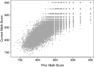
Figure 1 provides a scatterplot of current year versus prior year test scores for the students in our sample. The upper tails of the distributions exhibit the “stretching” commonly seen with scale scores in which raw scores for high-performing students convert to a few, spread out scale scores at the upper end of the scale. There are 55 unique values of the prior score, 54 unique values of the current score, and 1485 unique observed combinations of these prior and current scores. The data demonstrate relatively mild ceiling effects, with less than 0.5% of students reaching the highest possible prior year score, and about 1.6% of students reaching the highest possible current year score.

We consider three approaches to estimating the conditional CDFs and SGP. The first simply calculates the empirical CDF (ECDF) of the current score conditional on each possible prior score, and defines the “empirical SGP” to be the standard percentile rank of the current score in this conditional distribution, equal to the percentage of students scoring strictly less than a given student plus one half of the percentage of students scoring the same as the given student (Crocker and Algina 1986).² This definition ensures that the mean empirical SGP is exactly 50 for each possible prior score, and thus the marginal mean SGP is also exactly 50.

For the second estimation approach, we treated the outcome score as an ordered categorical variable with 54 levels and modeled the conditional probabilities as a function of the prior score using an ordered logit model. The model was implemented with the polr function in the MASS package for R. We used spline functions of the prior score in the model and used the Akaike information criterion (AIC) and likelihood ratio tests to choose the complexity. Both criteria suggested that a cubic spline with 6 degrees of freedom fit better than simpler models and was also preferred to a cubic spline with 7 degrees of freedom. The chosen model has a total of 59 parameters (6 for the coefficients on the spline basis for the prior score and 53 for the 54 ordered levels of the outcome). Analogous to the empirical SGP, we define the “logit SGP” as the estimated percentile rank of each student’s score given their prior score, which for each possible outcome score is the model-based estimate of the conditional probability of scoring strictly less than the observed score, plus one half the conditional probability of scoring exactly the observed score, all times 100.

Our third estimation approach used the studentGrowthPercentiles function in the SGP package³ for R based on 100 percentile cuts ranging from 0.5 to 99.5. The implied conditional CDFs from the model fit were calculated by manually inverting the estimated quantile functions, and the “standard SGP” is taken to be that returned by the function, calculated by comparing the current score for each student to the sequence of monotonized percentile cut points. The standard SGP approach here has a total of 800 parameters (7 for the coefficients on the spline basis for the prior score plus one for the intercept, times 100 quantile functions).

Figure 2 Estimated conditional CDFs (ECDF = black, logit model = blue, standard SGP approach = orange) for 502 students with prior score equal to 802. Kolmogorov–Smirnov (KS) statistics versus the ECDF are given in the legend.

Figure 3 Estimated conditional CDFs (ECDF = black, logit model = blue, standard SGP approach = orange) for 354 students with prior score equal to 890. Kolmogorov–Smirnov (KS) statistics versus the ECDF are given in the legend.

We first considered how well the estimated conditional CDFs from the ordered logit model and standard SGP approach recovered the conditional ECDFs, which in large samples would converge to the population conditional CDFs and thus would be appropriate for calculating SGP. Overall, the ordered logit model did a better job of recovering the ECDFs, which is not surprising because that model explicitly acknowledges the discreteness of the outcome. The two approaches performed similarly for the lower and middle parts of the prior score distribution, but the standard SGP approach started to do systematically worse in the upper part of the prior score distribution, where the outcome tended to take on fewer possible values.

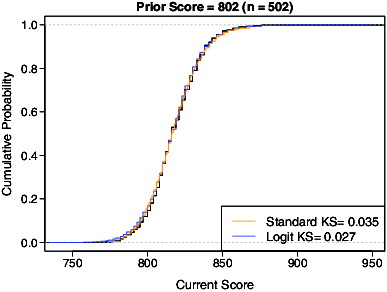
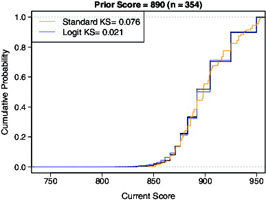
Figures 2 and 3 provide representative plots for two of the 55 unique prior scores. Each plot provides the estimated conditional CDFs from the three approaches, along with the Kolmogorov–Smirnov statistics (maximum absolute difference between CDFs) comparing the conditional CDFs from the ordered logit model and standard SGP approach to the conditional ECDFs. In Figure 2, corresponding to a prior score at approximately the 25th percentile, the conditional CDF estimated from the standard SGP approach (orange) is a very good approximation to the ECDF (black) because the sizes of the jumps in the conditional ECDF are relatively small. In Figure 3, for a prior score at about the 95th percentile, the impact of not directly dealing with the discreteness of the outcome distribution is more pronounced. The standard approach starts to exhibit flat spots, but they do not align as well with the conditional ECDF as the logit model (blue) does.

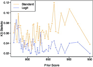
Figure 4 provides the Kolmogorov–Smirnov statistics of the conditional CDFs from the standard SGP approach (orange) and logit model (blue) relative to the conditional ECDFs, for each prior score with at least 50 students. For higher prior scores, the conditional CDFs for the standard SGP approach show consistently larger deviations from the conditional ECDFs than those from the logit model do, despite the fact that the conditional CDFs in the standard SGP approach are parameterized with significantly more parameters than the logit model. This behavior is probably not specific to our example and would not go away as the number of students becomes very large. It is likely that a model acknowledging the discreteness of the outcome—either standard ordered categorical models such as the logit model, or the less parametric conditional CDF approaches previously referenced—will tend to do a better job of recovering the conditional ECDFs than the standard SGP approach, particularly for outcome tests that have relatively few possible scale scores.

Figure 4 Kolmogorov–Smirnov (KS) statistics for the standard SGP approach (orange) and logit model (blue) versus the ECDF as a function of the prior score, for prior score values with at least 50 students.

This does not directly address how the estimated SGP will behave under different approaches. The SGP from the three different approaches have pairwise correlations exceeding 0.997, so at a gross level, the choice of model has negligible impact on estimated SGP. However, important differences can arise for subpopulations of students, and these differences can manifest at the teacher level when SGP are aggregated to MGP. The primary difference among the different approaches with respect to estimated SGP is in how ties in the outcome score are handled. There is no unambiguously correct choice. The percentile rank definition we used for the empirical and logit SGP has the property that in all circumstances, it gives students credit for exceeding the performance of half the students who share the same scale score. In other words, this percentile rank definition awards students “half credit” for students they tie. It is unclear whether this decision is correct or desirable, but it has the benefits of being a consistent convention and leading to SGP that will tend to have mean 50 regardless of how discrete the conditional distribution of the outcome is in a given comparison group. In contrast, the standard SGP is less uniform in its treatment of ties because the specific SGP values that it assigns depend on how the estimated quantile functions behave as the conditional distributions become more discrete in the extremes of the prior score distribution, where resolving individual quantiles becomes difficult. The exact behavior is difficult to predict given the complexity of the spline-based quantile regression models, and the deviations from “half credit” could be more or less pronounced in different circumstances.

Figure 5 Difference between the standard and empirical MGP (black triangles) and the difference between the logit and empirical MGP (gray circles) versus the average prior score of each teacher’s students, for teachers with at least 10 students.

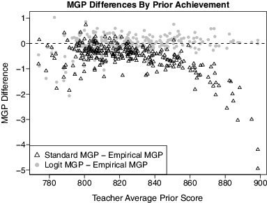
As an extreme example from our data, 89 students had the highest possible prior score. Thirty-eight (43%) of these students also had the highest possible current score. Each of these students had a standard SGP of 59, but empirical and logit SGP of approximately 79. The standard SGP gave these students effectively no credit for the students they tied. The behavior of the standard SGP in our data, which may be peculiar to these data, is to give students progressively less credit for ties as the prior score increases. That is, for students near the high end of the prior score distribution, the standard SGP tends to be systematically smaller than either the empirical or logit SGP. This implies that teachers teaching classrooms of very high achieving students will tend to receive MGP from the standard approach that are systematically smaller than what would be assigned from the other approaches.

Figure 5 displays the magnitudes of these differences in our data. Our data contained links of students to their grade 7 mathematics teachers, and we calculated MGP for each teacher by averaging the SGP for his/her linked students. The figure plots the difference between the standard and empirical MGP (black triangles) and the difference between the logit and empirical MGP (gray circles) versus the average prior score of each teacher’s students, for the 268 teachers with at least 10 students. As the average prior score of a teacher’s students increases, the standard MGP becomes systematically smaller than the empirical MGP, whereas the difference between the logit and empirical MGP appears to have no systematic relationship to the average prior score. The absolute differences are modest, but having any systematic differences as a result of an essentially arbitrary decision about how ties are handled may be viewed as problematic by stakeholders. Some teachers will be affected by the decision, and the amount individual teachers are affected will be related to the background characteristics of the students they teach.

Ties in the outcome score present a nuisance that transcends which statistical approach is used to estimate SGP. The primary advantage of directly modeling the conditional CDFs compared to the standard approach is that it is more straightforward to adopt a rule regarding ties and apply it uniformly to all students. This may be desirable given that one of the appeals of SGP and MGP approaches is simplicity and transparency.

An important limitation of our example is that because it was designed only to illustrate the ideas, we did not rigorously test the assumptions made by the ordinal logit model. It is possible that less rigid assumptions are more appropriate for either our data, or more generally. A key benefit of the standard SGP approach is that it makes minimal assumptions about the relationships among test scores, and that flexibility could be beneficial in some settings. It is also plausible that more flexible CDF modeling approaches, such as those noted previously, would provide a better framework for handling the peculiarities that can arise in joint distributions of longitudinal state testing data.

3. ESTIMATION FROM ITEM-LEVEL DATA

SGP from the standard approach and the CDF modeling approaches discussed in the previous section use distributions of observed test scores in a target population of students. However, observed test scores are error-prone measures of latent achievement (Lord 1980). Although SGP are formally only a descriptive statistic, in practice, they are interpreted as relative growth in achievement, and thus it is likely that the inference desired by consumers of SGP is more closely aligned with latent achievement than with observed test scores. For the remainder, we assume that the target SGP estimand involves the latent, true scores and their distributions rather than the observed scores and their distributions. We refer to this target SGP as the “latent SGP” to make explicit its definition in terms of the latent scores.

We let (X₀, X₁) be the latent achievement attributes measured with error by the observed test scores (W₀, W₁). We are defining (X₀, X₁) as hypothetical scores that result from letting the number of test items become large for the same tests administered at the same time to the same students as the actual tests. In this sense, the only source of measurement error we are addressing is that caused by the finite number of test items and the imperfect information about latent achievement provided by each item. We define the latent SGP as (2) $$\pi (X_0,X_1):=F_{X_1|X_0}\left(X_1\right|X_0)={\int }_{-\infty }^{X_1}{p}_{X_1|X_0}\left(u\right|X_0)du.$$(2) Comparing Equation (2(2) $$\pi (X_0,X_1):=F_{X_1|X_0}\left(X_1\right|X_0)={\int }_{-\infty }^{X_1}{p}_{X_1|X_0}\left(u\right|X_0)du.$$(2) ) to (1(2) $$\rho (W_0,W_1):=F_{W_1|W_0}\left(W_1\right|W_0)={\int }_{-\infty }^{W_1}{p}_{W_1|W_0}\left(u\right|W_0)du,$$(2) ) shows that the definitions are parallel, but one is defined in terms of latent scores and distributions (Equation (2(2) $$\pi (X_0,X_1):=F_{X_1|X_0}\left(X_1\right|X_0)={\int }_{-\infty }^{X_1}{p}_{X_1|X_0}\left(u\right|X_0)du.$$(2) )) and the other in terms of observed scores and distributions (Equation (1(2) $$\rho (W_0,W_1):=F_{W_1|W_0}\left(W_1\right|W_0)={\int }_{-\infty }^{W_1}{p}_{W_1|W_0}\left(u\right|W_0)du,$$(2) )). We denote the latent SGP as π(X₀, X₁) and the “observed SGP” as ρ(W₀, W₁).

3.1 Potential Issues With the Standard Approach

Due to the nonlinearity of the steps used to compute SGP, it is generally the case that a student’s observed SGP is a biased estimator of his or her latent SGP, even if each test score used in the calculation is an unbiased estimate of the latent achievement construct it is intended to measure. That is, E[ρ(W₀, W₁)|X₀, X₁] is not generally equal to π(X₀, X₁). In fact, even if the SGP could be calculated using the latent values of past achievement, measurement error in the current year score alone would be sufficient to cause bias in the SGP due to the nonlinear functions used to calculate SGP. For example, if the measurement error variance in the current score was very large, the observed SGP would be dominated by measurement error and would have mean near 50 (i.e., the median percentile rank) regardless of the true SGP.

The potential for bias in inferences from SGP stemming from test measurement error may be exacerbated for school or teacher MGP. Because students in different schools and different teachers’ classes are likely to differ with respect to latent achievement, errors in student SGP caused by test score measurement error that are systematically related to latent achievement will not cancel when aggregated. This can result in systematic errors in MGP for teachers or schools that are correlated with the students’ background characteristics. Because MGP are sometimes interpreted as indicators of relative effectiveness of schools or teachers, this can lead to certain teachers or schools being chronically advantaged or disadvantaged by the evaluation metrics depending on the types of students they serve. The potential for such systematic error has been raised and studied in the broader literature on teacher value-added for more than a decade (McCaffrey et al. 2003; Rothstein 2010; Harris 2011; Kane et al. 2013). This was also a major issue with MGP noted by both the Guarino et al. and Walsh and Isenberg articles.

Dealing with test measurement error in the standard SGP approach is very difficult. As noted previously, the algorithmic computation of SGP makes it unclear how to apply any standard measurement error correction approaches. Shang, Van Iwaarden, and Betebenner (2014) provided an initial attempt to address measurement error in the conditioning scores used in SGP by using SIMEX. However, the methods in that study are insufficient to fully correct for bias in SGP induced by measurement error. Also, there have been no methods proposed to address the bias in SGP due to measurement error in the current (outcome) test score.

3.2 Potential Improvements

Correcting SGP (and thus MGP) for measurement error in both past and current scores, that is, developing estimators for the latent SGP π(X₀, X₁) in Equation (2(2) $$\pi (X_0,X_1):=F_{X_1|X_0}\left(X_1\right|X_0)={\int }_{-\infty }^{X_1}{p}_{X_1|X_0}\left(u\right|X_0)du.$$(2) ), would be relatively straightforward if the SGP estimation process started with the item-level data. States have access to such item-level data, and standard methods based on MIRT exist for the steps required to go from longitudinal item-level data to latent SGP estimators.

The estimation problem parallels that faced by testing programs in using item-level data from a single test to estimate each student’s latent achievement. However, the SGP case presents two specific challenges: (i) the target parameter π(X₀, X₁) involves two latent achievement values and (ii) the target parameter is a nonlinear function of those latent achievement values that is defined only in reference to the distribution of latent achievement in some target population, which itself must be estimated from the observed data. These problems have been studied in the literature in other contexts than SGP, and we next discuss how those solutions could be applied to the estimation of SGP.

3.2.1 Estimating Latent Score Distributions

The first challenge to estimating π(X₀, X₁) is that it requires estimating the conditional distributions of the latent scores in the target population from the observed item response data. These conditional distributions would follow directly from an estimate of the joint distribution $p_{X_0,X_1}(x_0,x_1)$ in the target population. This is the well-studied problem of deconvolution of a latent distribution given error-prone measures (Laird 1978; Mislevy 1984; Roeder, Carroll, and Lindsay 1996; Rabe-Hesketh, Pickles, and Skrondal 2003; Carroll et al. 2006; Lockwood and McCaffrey 2014). Deconvolution methods use the fact that the item response theory model (IRT; see, e.g., van der Linden and Hambleton 1996 or Holland 1990) defines the probability structure of the observed item responses conditional on the latent scores, and therefore the observed item response distributions can be used to infer the latent score distributions.

We propose that states could use the longitudinal item response data on individual students to estimate bivariate IRT models that would provide an estimate of $p_{X_0,X_1}(x_0,x_1)$ in the target population. The target population would be restricted to a subset of the full student population having some minimum threshold of longitudinal data; in the simplest case, the estimation would be restricted to students having two consecutive years of test scores. Software available for MIRT, such as flexMIRT (Cai 2012), the mdltm program for multidimensional discrete latent trait models (von Davier 2005), the MIRT routines by Haberman (2013) or Glas (2010), or packages available in R such as mirt (Chalmers, Pritikin, and Zoltak 2014), could be used to perform the estimation under different assumptions about $p_{X_0,X_1}(x_0,x_1)$.

These assumptions range from highly parametric to nonparametric, and the key question for the SGP application is how much parametric structure is required to estimate $p_{X_0,X_1}(x_0,x_1)$ in such a way that the conditional distributions are reasonably smooth and well identified from the available data. Fully nonparametric approaches to deconvolution (Roeder, Carroll, and Lindsay 1996; Rabe-Hesketh, Pickles, and Skrondal 2003) tend to result in distributions that are not smooth and may not provide consistent estimators for IRT models depending on the complexity of the item response function (Haberman 2005a). Therefore, parametric assumptions will likely be required in practice to obtain well-behaved estimates of the latent bivariate distribution. It is possible that the standard MIRT assumption of bivariate normality of (X₀, X₁) would fit the data sufficiently well, because much of the evident deviation of observed scores from bivariate normality is likely due to heteroscedastic measurement error present in the observed scores but not the latent scores. Parametric extensions of the multivariate normal family that allow for skewness are also available (Azzalini and Dalla Valle 1996) and could be tested against the standard normality assumption, as could mixtures of normal distributions. Latent class models that assume a discrete latent distribution are also possible and may provide good approximations to an underlying continuous distribution (Haberman 2005b; Haberman, von Davier, and Lee 2008; Xu and von Davier 2008). Empirical investigations with test score data from state testing programs would be needed to strike the right balance between being flexible enough to capture the real structure but being parameterized enough to provide reasonable distribution estimates.

3.2.2 Estimating Individual SGP

Given an estimate ${\widehat{p}}_{X_0,X_1}(x_0,x_1)$, there is still the problem of how to estimate the SGP for each student given his or her item responses (I₀, I₁) on the two tests. This problem is isomorphic to how item responses from a single test are used to estimate the latent achievement for that test. Different estimators have different advantages and disadvantages, and here we highlight only a few key issues.

If the item parameters of the MIRT model were known, each student’s (X₀, X₁) can be estimated by maximum likelihood (MLE) given (I₀, I₁). The MLE SGP would follow from plugging these estimates into the π function from Equation (2(2) $$\pi (X_0,X_1):=F_{X_1|X_0}\left(X_1\right|X_0)={\int }_{-\infty }^{X_1}{p}_{X_1|X_0}\left(u\right|X_0)du.$$(2) ) if the latent achievement distribution was also known. In practice, both the item parameters and the latent achievement distribution would be estimated from the observed data, typically by marginal maximum likelihood (Bock and Aitkin 1981; Baker and Kim 2004). The MLEs of the achievement attributes would then be calculated conditional on the estimated item parameters, and the MLE SGP would be based on the $\widehat{\pi }$ function determined from ${\widehat{p}}_{X_0,X_1}(x_0,x_1)$. The MLE SGP h(I₀, I₁) would be approximately unbiased for large numbers of items and students in the sense that a student with latent achievement (X₀, X₁) would have E[h(I₀, I₁)|X₀, X₁] ≈ π(X₀, X₁), where the expectation is over the distribution of item responses conditional on latent achievement. The primary limitations of the MLE SGP are that it is not defined for students responding to all of the questions either correctly or incorrectly on one or both of the tests, and it has small-sample bias related to the number of test items. It may be possible to remedy both issues by using weighted likelihood estimation (WLE; Warm 1989; Wang 2014), but further study would be required to determine whether plugging the WLE estimate for each test into $\widehat{\pi }$ would achieve the bias reduction that WLE provides for each individual latent attribute, or whether an alternative WLE approach specifically tailored to the estimation of the latent SGP would be required.

The fact that the MLE does not always exist can also be avoided by using empirical Bayes’ estimation of π(X₀, X₁) given (I₀, I₁). Again, in practice, marginal maximum likelihood would commonly be used to estimate both the item parameters and the latent achievement distribution, which directly provide the empirical Bayes’ posterior of π(X₀, X₁) given (I₀, I₁). The posterior mean or expected a posteriori (EAP) SGP E[π(X₀, X₁)|I₀, I₁] would be an obvious choice for a point estimator and does not suffer the same existence problems as the MLE SGP. This estimator would not be unbiased, but would be calibrated in the sense that students with a given value of E[π(X₀, X₁)|I₀, I₁] would, on average over their corresponding distributions of latent scores, have latent SGP equal to E[π(X₀, X₁)|I₀, I₁]. The main downside of the EAP SGP is that it is a shrunken estimate and therefore is underdispersed relative to the true SGP distribution. Because schools or teachers are not accounted for during the SGP estimation, the MGP estimators for schools or teachers created by aggregating the EAP SGP will be biased toward 50, which might be viewed as undesirable by some stakeholders. Therefore choosing among MLE, EAP, or other estimation approaches for individual SGP when item-level data are modeled directly requires further scrutiny.

One of the main advantages of estimating SGP using the item-level data is that the different candidate estimators have corresponding measures of uncertainty that can be calculated using standard methods. The impact of uncertainty in the estimated latent population distribution and its conditional distributions, as well as in the item parameters from the MIRT model, would be most straightforwardly addressed in a fully Bayesian analysis where the latent distribution was parameterized or otherwise given a prior distribution along with the item parameters (Patz and Junker 1999). In this case, the posterior distribution of the SGP would simultaneously account for uncertainty about the population distribution of latent achievement, item parameters, and each student’s latent achievement. However, given that SGP applications typically will use an entire state’s worth of data, uncertainty in the estimated population distribution and item parameters may contribute negligibly to the uncertainty in SGP, making empirical Bayesian approaches potentially satisfactory.

4. CONCLUDING REMARKS

Due to their intuitive appeal and minimal reliance on scale assumptions, SGP are positioned to grow as part of education research, practice, and reporting. The ideas presented here may help to avoid the nuisances to the standard estimation approach caused by test measurement error and the discreteness of the observed scores. Both of our suggested alternative approaches would need substantial development and would need to be carefully compared against the standard approach with real data to fully understand the costs and benefits. Such research is beginning to emerge; as this article was going to press, a report by Monroe, Cai and Choi (2014) was released that conducts empirical and simulated evaluations of SGP estimators based on MIRT models.

It is important to note that our suggestions do not address some of the key limitations of SGP that exist regardless of how they are estimated. The first is that SGP are intrinsically normative, and thus do not provide information about achievement progress in absolute terms. Both the standard SGP approach and our suggested alternatives place students on a continuum of relative achievement status conditional on past achievement without regard to whether the progress of a typical student is adequate, or otherwise meets expectations of the education system. Thus, SGP or MGP alone, regardless of how they are estimated, are insufficient to gauge whether students are learning what they are expected to learn.⁴

Another major concern is that SGP are inherently limited by a lack of reliability. Given the generally high correlations of test scores within students over time and the measurement error in each test used in the SGP calculation, much of the observed variation across students in SGP will be due to measurement error, regardless of how SGP are calculated. Correcting the bias in SGP due to test measurement error does not fix this problem. Confidence intervals or other measures of uncertainty in individual SGP are likely to cover a large portion of the percentile rank range for many students, and precision is not likely to be markedly improved even with statistical approaches tuned to the SGP estimation problem, such as those discussed here. It is thus unclear whether SGP, or any other student-level growth statistic based on typical test scores, is sufficiently reliable to support consequential decision making for individual students.

The lack of reliability of SGP at the student level is mitigated when aggregating to higher levels with MGP. However, as noted by Guarino et al. (2014) and Walsh and Isenberg (2014) among others, MGP will generally provide biased estimates of educator performance when teachers of different effectiveness systematically teach students of different prior achievement levels. This bias is a consequence of the fact that teachers and schools are not accounted for during SGP estimation. Neither of the suggestions made here address this issue, although modifications to those approaches or to the standard approach to address the issue are possible. For example, indicator variables for individual schools or teachers could be included in conditional CDF models, in quantile regression models, or in ordered categorical models. They could also be included in the latent structure specified inside MIRT models (i.e., latent regression), analogous to the approach used in the National Assessment of Educational Progress (Mislevy, Johnson, and Muraki 1992). This could mitigate the bias problem for MGP but further blurs the line between MGP and value-added methods, and damages the conceptual simplicity of SGP methods that provide an interpretable student-level statistic that can be aggregated transparently to higher levels. It remains an open question whether a procedure can be developed that satisfies the goals of minimal reliance on scaling assumptions, transparency, and simplicity of explanation to nontechnical audiences, and approximately unbiased estimates of both relative student growth and educator performance.

FUNDING

The research reported here was supported in part by the Institute of Education Sciences, U.S. Department of Education, through Grant R305D140032 to ETS. The opinions expressed are those of the authors and do not represent views of the Institute or the U.S. Department of Education.

Additional information

Notes on contributors

J. R. Lockwood

J. R. Lockwood is a Principal Research Scientist at Educational Testing Service, Princeton, NJ 08541 (E-mail: [email protected]). Katherine E. Castellano is an Associate Psychometrician at Educational Testing Service, San Francisco, CA 94105 (E-mail: [email protected]). The ideas presented here benefited significantly from conversations with Shelby J. Haberman and Daniel F. McCaffrey. The authors thank Rebecca Zwick, Matthias von Davier, and Johnny Lin for constructive comments on an earlier draft of the article.

Katherine E. Castellano

J. R. Lockwood is a Principal Research Scientist at Educational Testing Service, Princeton, NJ 08541 (E-mail: [email protected]). Katherine E. Castellano is an Associate Psychometrician at Educational Testing Service, San Francisco, CA 94105 (E-mail: [email protected]). The ideas presented here benefited significantly from conversations with Shelby J. Haberman and Daniel F. McCaffrey. The authors thank Rebecca Zwick, Matthias von Davier, and Johnny Lin for constructive comments on an earlier draft of the article.

Notes

The technical descriptions of SGP (e.g., Betebenner 2008, 2009) do not mention how monotonicity is ensured, but the documentation of the SGP package (Betebenner et al. 2014) states that monotonicity constraints are enforced using the methods of Dette and Volgushev (2008). However, it was difficult to reconcile those methods with what is implemented in the SGP package, which appears to be for each student, simply resorting the 100 estimated conditional quantiles so that they are nondecreasing. This is more consistent with the suggestions of Chernozhukov, Fernandez-Val, and Galichon (2009, 2010) than with those of Dette and Volgushev (2008), as confirmed by personal communication with Damian Betebenner on July 14, 2014.

This formula for percentile ranks is used more broadly in educational measurement applications, including in equipercentile equating or linking; Kolen and Brennan 2004, pp. 38–39.

The SGP package was version 1.2-0.0 (Betebenner et al. 2014) for R version 3.0.2 running on i386 Linux.

We note that Betebenner (2009) extended SGP to percentile growth trajectories to afford criterion-referenced growth-to-standard interpretations, but SGP in and of themselves do not afford such interpretations, and this extension involves further assumptions that may be problematic.

REFERENCES

- Agresti, A. (1990), Categorical Data Analysis, New York: Wiley.
- Azzalini, A., Dalla Valle, A. (1996), “The Multivariate Skew-Normal Distribution, Biometrika, 83, 715–726.
- Baker, F., and Kim, S. (2004), Item Response Theory: Parameter Estimation Techniques ( 2nd ed.), New York: Marcel-Dekker.
- Betebenner, D. (2008), “A Primer on Student Growth Percentiles, Technical Report, National Center for the Improvement of Educational Assessment. Available at https://www.gadoe.org/Curriculum-Instruction-and-Assessment/Assessment/Documents/Aprimeronstudentgrowthpercentiles.pdf
- ——— (2009), “Norm- and Criterion-Referenced Student Growth, Educational Measurement: Issues and Practice, 28, 42–51.
- ——— (2011), “A Technical Overview of the Student Growth Percentile Methodology: Student Growth Percentiles and Percentile Growth Projections/Trajectories, Technical Report, National Center for the Improvement of Educational Assessment, Dover, NH. Available at http://www.nj.gov/education/njsmart/performance/SGP_Technical_Overview.pdf.
- Betebenner, D., Van Iwaarden, A., Domingue, B., and Shang, Y. (2014), SGP: An R Package for the Calculation and Visualization of Student Growth Percentiles & Percentile Growth Trajectories, R package version 1.2-0.0. Available at http://centerforassessment.github.com/SGP/
- Bock, R., Aitkin, M. (1981), “Marginal Maximum Likelihood Estimation of Item Parameters: Application of an EM Algorithm, Psychometrika, 46, 443–459.
- Breslow, N.E. (1972), “Discussion of “Regression Models and Life Tables,” by D.R Cox, Journal of the Royal Statistical Society, Series B, 34, 216–217.
- Briggs, D., and Betebenner, D. (2009), “Is Growth in Student Achievement Scale Dependent?” Paper Presented at the Annual Meeting of the National Council for Measurement in Education, San Diego, CA.
- Brunel, E., Comte, F., Lacour, C. (2010), “Minimax Estimation of the Conditional Cumulative Distribution Function, Sankhya A, 72, 293–330.
- Cai, L. (2012), flexMIRT: Flexible Multilevel Item Factor Analysis and Test Scoring, Seattle, WA: Vector Psychometric Group, LLC.
- Carroll, R., Ruppert, D., Stefanski, L., and Crainiceanu, C. (2006), Measurement Error in Nonlinear Models: A Modern Perspective ( 2nd ed.), London: Chapman and Hall.
- Castellano, K.E., Ho, A.D. (2013), “Contrasting OLS and Quantile Regression Approaches to Student “Growth” Percentiles, Journal of Educational and Behavioral Statistics, 38, 190–215.
- ——— (2014), “Practical Differences Among Aggregate-Level Conditional Status Metrics: From Median Student Growth Percentiles to Value-Added Models, Journal of Educational and Behavioral Statistics.DOI: 10.3102/1076998614548485.
- Chalmers, P., Pritikin, J., and Zoltak, M. (2012), “mirt: An R Package for Multidimensional Item Response Theory,” Journal of Statistical Software, 48, 1–29.
- Chernozhukov, V., Fernandez-Val, I., Galichon, A. (2009), “Improving Point and Interval Estimators of Monotone Functions by Rearrangement, Biometrika, 96, 559–575.
- ——— (2010), “Quantile and Probability Curves Without Crossing, Econometrica, 78, 1093–1125.
- Colorado Department of Education, (2013), Measures of Student Learning Guidance for Districts: Version 2.0, Denver, CO: Colorado Department of Education. Available at http://www.cde.state.co.us/sites/default/files/MeasuresofStudentLearningFIN AL081413.pdf.
- Cook, J., Stefanski, L. (1994), “Simulation-Extrapolation Estimation in Parametric Measurement Error Models, Journal of the American Statistical Association, 89, 1314–1328.
- Cox, D. (1972), “Regression Models and Life Tables ( with discussion), Journal of the Royal Statistical Society, . Series B, 34, 187–220.
- ——— (1975), “Partial Likelihood, Biometrika, 62, 269–276.
- Crocker, L., and Algina, J. (1986), Introduction to Classical and Modern Test Theory, Orlando, FL: Holt, Rinehart and Winston.
- Dette, H., Volgushev, S. (2008), “Non-Crossing Non-Parametric Estimates of Quantile Curves, Journal of the Royal Statistical Society, Series B, 70, 609–627.
- Georgia Department of Education, (2014), Leader Keys Effectiveness System: Implementation Handbook, Georgia Department of Education. Available at http://www.gadoe.org/School-Improvement/Teacher-and-Leader-Effectiveness/Documents/FY15%20TKES%20and%20LKES%20Documents/LKES%20Handbook-%20%20FINAL%205-30-14.pdf
- Glas, C. (2010), “Preliminary Manual of the Software Program Multidimensional Item Response Theory (MIRT), technical report, University of Twente, The Netherlands. Available at http://www.utwente.nl/gw/omd/Medewerkers/temp_test/mirt-manual.pdf
- Guarino, C.M., Reckase, M.D., Stacy, B.W., Wooldridge, J.M. (2014), “A Comparison of Growth Percentile and Value-Added Models of Teacher Performance, Statistics and Public Policy.
- Haberman, S. (1979), Analysis of Qualitative Data ( Vols. 1 and 2), New York: Academic Press.
- Haberman, S. (2013), “A General Program for Item-Response Analysis That Employs the Stabilized Newton-Raphson Algorithm, ETS Research Report No. RR-13-32. Princeton, NJ: Educational Testing Service.
- Haberman, S. (2005a), “Identifiability of Parameters in Item Response Models With Unconstrained Ability Distributions, ETS Research Report No. RR-05-24. Princeton, NJ: Educational Testing Service.
- Haberman, S. (2005b), “Latent-Class Item Response Models, ETS Research Report. No. RR-05-28. Princeton, NJ: Educational Testing Service.
- Haberman, S.J., von Davier, M., Lee, Y. (2008), “Comparison of Multidimensional Item Response Models: Multivariate Normal Ability Distributions Versus Multivariate Polytomous Distributions, ETS Research Report No. RR-08-45. Princeton, NJ: Educational Testing Service.
- Hall, P., Wolff, R.C., Yao, Q. (1999), “Methods for Estimating a Conditional Distribution Function, Journal of the American Statistical Association, 94, 154–163.
- Hansen, B.E. (2004), “Nonparametric Estimation of Smooth Conditional Distributions,” unpublished manuscript, Department of Economics, University of Wisconsin.
- Harris, D. (2011), Value-Added Measures in Education: What Every Educator Needs to Know, Cambridge, MA: Harvard Education Press.
- Holland, P. (1990), “On the Sampling Theory Foundations of Item Response Theory Models, Psychometrika, 55, 577–601.
- Kalbfleisch, J.D., Prentice, R.L. (1973), “Marginal Likelihoods Based on Cox’s Regression and Life Model, Biometrika, 60, 267–278.
- ——— (2002), The Statistical Analysis of Failure Time Data 2, New York: Wiley.
- Kane, T., McCaffrey, D., Miller, T., Staiger, D. (2013), “Have We Identified Effective Teachers? Validating Measures of Effective Teaching Using Random Assignment, Bill and Melinda Gates Foundation MET Project Research Paper.
- Koenker, R. (2005), Quantile Regression, London: Cambridge University Press.
- Kolen, M., and Brennan, R. (2004), Test Equating, Scaling, and Linking, New York: Springer.
- Laird, N. (1978), “Nonparametric Maximum Likelihood Estimation of a Mixing Distribution, Journal of the American Statistical Association, 73, 215–232.
- Li, Q., Lin, J., Racine, J.S. (2013), “Optimal Bandwidth Selection for Nonparametric Conditional Distribution and Quantile Functions, Journal of Business & Economic Statistics, 31, 57–65.
- Li, Q., and Racine, J.S. (2007), Nonparametric Econometrics: Theory and Practice, Princeton, NJ: Princeton University Press.
- ——— (2008), “Nonparametric Estimation of Conditional CDF and Quantile Functions With Mixed Categorical and Continuous Data, Journal of Business & Economic Statistics, 26, 423–434.
- Lockwood, J., McCaffrey, D. (2014), “Correcting for Test Score Measurement Error in ANCOVA Models for Estimating Treatment Effects, Journal of Educational and Behavioral Statistics, 39, 22–52.
- Lord, F. (1980), Applications of Item Response Theory to Practical Testing Problems, Hillsdale, NJ: Lawrence Erlbaum Associates.
- McCaffrey, D., Lockwood, J., Koretz, D., and Hamilton, L. (2003), Evaluating Value-Added Models for Teacher Accountability, (MG-158-EDU), Santa Monica, CA: RAND.
- McCullagh, P. (1980), “Regression Models for Ordinal Data, Journal of the Royal Statistical Society, Series B, 42, 109–142.
- Mislevy, R.J. (1984), “Estimating Latent Distributions, Psychometrika, 49, 359–381.
- Mislevy, R.J., Johnson, E., Muraki, E. (1992), “Scaling Procedures in NAEP, Journal of Educational Statistics, 17, 131–154.
- Monroe, S., Cai, L., and Choi, K. (2014), Student Growth Percentiles Based on MIRT: Implications of Calibrated Projection, (CRESST Report 842), Los Angeles, CA: University of California, National Center for Research on Evaluation, Standards, and Student Testing (CRESST).
- Patz, R.J., Junker, B.W. (1999), “A Straightforward Approach to Markov Chain Monte Carlo Methods for Item Response Models, Journal of Educational and Behavioral Statistics, 24, 146–178.
- Prentice, R.L., Gloeckler, L.A. (1978), “Regression Analysis of Grouped Survival Data With Application to Breast Cancer Data, Biometrics, 34, 57–67.
- Rabe-Hesketh, S., Pickles, A., Skrondal, A. (2003), “Correcting for Covariate Measurement Error in Logistic Regression Using Nonparametric Maximum Likelihood Estimation, Statistical Modelling, 3, 215–232.
- R Development Core Team (2013), R: A Language and Environment for Statistical Computing, Vienna, Austria: R Foundation for Statistical Computing.
- Reckase, M. (2009), Multidimensional Item Response Theory, New York: Springer.
- Roeder, K., Carroll, R., Lindsay, B. (1996), “Nonparametric Maximum Likelihood Estimation of a Mixing Distribution, Journal of the American Statistical Association, 91, 722–732.
- Rothstein, J. (2010), “Teacher Quality in Educational Production: Tracking, Decay, and Student Achievement, Quarterly Journal of Economics, 125, 175–214.
- Shang, Y. (2012), “Measurement Error Adjustment Using the SIMEX Method: An Application to Student Growth Percentiles, Journal of Educational Measurement, 49, 446–465.
- Shang, Y., Van Iwaarden, A., and Betebenner, D. (2014), “Measurement Error Correction for the Student Growth Percentile Model,” Paper Presented at National Council on Measurement in Education Annual Research Conference, Philadelphia, PA.
- van der Linden, W., and Hambleton, R. (1996), Handbook of Modern Item Response Theory, New York: Springer-Verlag.
- von Davier, M. (2005), “A General Diagnostic Model Applied to Language Testing Data, ETS Research Report No. RR-05-16. Princeton, NJ: Educational Testing Service.
- Walsh, E., Isenberg, E. (2014), “How Does a Value-Added Model Compare to the Colorado Growth Model? Statistics and Public Policy.
- Wang, C. (2014), “On Latent Trait Estimation in Multidimensional Compensatory Item Response Models, Psychometrika, DOI: 10.1007/s11336-013-9399-0
- Warm, T. (1989), “Weighted Likelihood Estimation of Ability in the Item Response Theory, Psychometrika, 54, 427–450.
- Xu, X., von Davier, M. (2008), “Fitting the Structured General Diagnostic Model to NAEP Data, ETS Research Report No. RR-08-27, Princeton, NJ: Educational Testing Service.