Childhood Brain Cancer in Florida: A Bayesian Clustering Approach

Abstract

In this article, we focus on geocoded data for pediatric brain cancer in Florida. Specifically, we examine zip code level pediatric brain cancer counts from the Florida Association of Pediatric Tumor Programs (FAPTP) childhood cancer registry from 2000–2010 and assess the degree of spatial clustering in these data. We assume Bayesian models for relative risk and examine a variety of posterior measures that indicate excess risk (exceedence probability of relative risk or positive residual). We assume a standard Poisson convolution model and examine a zero-inflated (ZI) model with a factored intercept. We conclude that there is evidence of excess risk in a number of relatively dispersed zip codes across the state but there appears to be some concentration of high excess risk in Polk, Lake, and Sumter counties (west of Orlando and north east of Tampa). These excesses are confirmed across the models.

KEY WORDS::

• Exceedence probability
• Florida zip code
• Pediatric brain cancer
• Relative risk

View correction statement:

Corrigendum

1. INTRODUCTION

Incidence of childhood brain cancer has been of concern in the U.S. State of Florida. A recent publication (Lawson 2014) has highlighted the existence of putative clusters of pediatric brain cancer at zip code aggregation level in this U.S. state. In particular, the raised incidence of pediatric brain cancer was found in the southern area of the state (south Florida cluster). There is a perceived need for further analysis to assess the robustness of the findings under different assumptions.

Cancer cluster investigations can be highly focused and have defined locations or areas where clustering is to be measured (Lawson 2014) or can provide an overview of a general cluster tendency in a province or state. This latter situation is known as nonfocused clustering. In nonfocused clustering no apriori idea of clustering tendency is assumed and so it is usually felt that a reasonably flexible and lowly parameterized method would be best employed to allow the data “to speak.” In the case of the state of Florida and brain cancer registry cases in zip codes, we have a nonfocused clustering scenario whereby we assume no previous knowledge of locations of clusters and so we do not employ techniques that would be pertinent to focused investigations (Lawson 2006, Chap. 6).

However, it is also important to define the nature of the clusters or clustering to be studied. There are a variety of definitions of clusters and different definitions will lead to differences in the ability to detect clusters. In this article, there are two main scenarios of clustering to be considers: hot spot and cluster. A hot spot is an isolated area with excess risk. A cluster is a group of neighbor areas with an excessive relative risk(Lawson 2014).

2. STUDY AREA AND POPULATION

Our study area is defined at the zip code level and data are available for the period 2000–2010. We decided to use the 983 Florida zip code areas defined as zip code tabulation areas (ZCTAs) in 2010 as geographical units in the analysis. For each zip code, the population at risk includes the entire population of 0–19 years of age in the state of Florida during the time period 2000–2010. The case information is available through the Florida Association of Pediatric Tumor Programs (FAPTP) (Amin et al. 2010). These data consist of all recorded brain cancer within the registry for that time period. Many ZCTAs were found to have no cases during this period and these were allocated a zero count so that all ZCTAs had a complete enumeration of cases.

3. DATA ANALYSES

3.1 Models

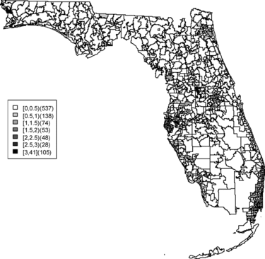
In this article, zip code areas are denoted as i = 1, …, m where y_i and e_i respectively denote the number of cases and expected number of cases within the ith area. The expected rates are calculated as where y^p_i is the population in the ith area in the state of Florida during time period 2000–2010. The sum is over all ZCTAs in the study region. A commonly made assumption is that the case counts are independently distributed Poisson variates, that is, y_i ∼ Poisson(μ_i), and μ_i = e_iθ_i where θ_i is a relative risk parameter for the ith area. The estimate of the relative risk of area i is the saturated maximum likelihood estimator and is known as the standardized morbidity ratio (SMR) which is defined as SMR_i = y_i/e_i. Although this estimate is well known and easy to compute, it can be misleading, particularly applied to rare diseases, as zero counts lead to undifferentiated SMRs and “close-to-zero” expected counts can lead to very large SMRs regardless of the observed count. However, the SMR can be employed to obtain an exploratory view of how disease rates or clusters distribute over the study area. The map of SMRs for each zip code is shown in Figure 1. The SMR map contains much confounding noise and we pursue more reliable relative risk estimates. More reliable estimates of relative risks for rare diseases for small areas can be obtained by borrowing information from neighboring areas. A way to capture the relationship between the neighborhoods is to use hierarchical modeling which includes neighborhood information and this setting can be naturally dealt with in a Bayesian framework.

Figure 1. The standardized morbidity ratio of the childhood cancer data at each zip code area.

The Besag, York, and Mollie (BYM) model (Besag, York, and Mollié 1991) has been shown in many studies to yield robust estimates across a range of scenarios including clustering of disease (Best, Richardson, and Thomson 2005; Lawson 2013; Rotejanaprasert 2014). The model decomposes the log of area-level relative risks into the sum of two random effects: one which is unstructured (heterogeneous), v_i, and the other spatially structured (dependent), u_i. The unstructured random effects are assumed to follow a zero-mean normal distribution. The spatially structured effects are modeled by the intrinsic conditional autoregressive normal (ICAR) prior distribution. In simple formulation, the prior distribution can be specified as the conditional distribution of each area-specific spatially structured effect, given all other spatial effects, and is a normal distribution with mean equal to the average of its neighbors, and precision proportional to the number of these neighbors. The neighborhood set for the ith area is δ_i and the number of neighbors is . This means that the precision increases as the number of neighbors increases. Then, the model can be expressed as

Table 1. Model comparisons for the childhood cancer data using BYM and SPC models

	DIC	pD	WAIC	pWAIC	MSPE
BYM	2541	324.8	1418.9	269.1	2.362
SPC	2078	217.1	1123.1	186.3	2.361

Each of the main terms on the BYM model has a Gaussian prior distribution and their precisions are modeled via the stable SD-uniform specification above (Gelman 2006). This model is also known as a convolution model and is commonly applied for relative risk estimation with small area health data.

Table 2. Zip code areas with the lowest (left) and highest (right) relative risks of the BYM model

zip code	relative risk	zip code	relative risk
34,771	0.04318	32,625	10.35
34,224	0.04804	34,201	8.53
34,228	0.05152	32,130	8.024
32,818	0.3726	32,801	7.223
32,304	0.3776	32,501	6.51
32,703	0.3806	32,568	6.497
33,610	0.3872	32,202	6.386
33,578	0.4045	32,456	6.042
34,758	0.4049	32,131	5.773
33,810	0.4207	33,931	5.622
33,615	0.4214	32,730	5.441
32,811	0.4254	33,316	5.175
34,116	0.4317	32,145	4.482
33,619	0.4433	32,901	4.407
34,743	0.4433	32,443	4.37
33,186	0.4509	33,760	4.252
32,244	0.452	32,618	4.126
34,221	0.4547	32,053	4.048
33,411	0.4549	32,058	3.975
32,909	0.463	32,421	3.755

Table 3. Zip code areas with the lowest (left) and highest (right) relative risks of the SPC model

zip code	relative risk	zip code	relative risk
32,811	7.73E-04	32,625	6.838
33,904	7.79E-04	32,130	6.64
32,334	7.80E-04	34,201	6.133
34,449	7.82E-04	32,801	5.972
32,949	7.90E-04	32,501	5.679
34,434	7.93E-04	32,568	5.312
34,450	7.96E-04	32,202	5.251
33,187	7.96E-04	32,456	5.216
32,827	7.97E-04	32,131	4.924
33,839	7.98E-04	32,730	4.669
32,061	7.99E-04	33,931	4.623
32,970	7.99E-04	33,316	4.487
33,146	8.00E-04	32,901	4.179
34,681	8.02E-04	33,760	4.082
32,833	8.03E-04	32,145	3.981
34,240	8.03E-04	32,443	3.849
32,003	8.04E-04	32,618	3.695
34,758	8.04E-04	32,058	3.673
32,311	8.04E-04	32,053	3.599
32,212	8.06E-04	33,936	3.548

Since childhood cancer is a rare disease, there are zip code areas with no cases. This sparseness of the count outcomes can be a problem as the Poisson data level model might not be able to model the situation where there can be multimodality in the marginal count distribution. The presence of a large amount of zeroes in the data often leads to the consideration of zero-inflated (ZI) models such as the zero-inflated Poisson (ZIP) model which is often employed (Cheung 2002; Lawson 2013). ZIP models have been reviewed in Ghosh et al. (Ghosh, Mukhopadhyay, and Lu 2006). Song et al. (Song et al. 2011) proposed a simpler variant of a ZIP model whereby the zero counts have a separate intercept. This model is known as the sparse Poisson convolution (SPC) and it is used to model geographic variation in rare diseases. It has been found to outperform certain ZIP models in the original study. Rather than modeling the data as a mixture model of zeroes and a Poisson distribution as in the ZIP models, the SPC approach decomposes as two Poisson components of zero and nonzero counts. To employ this model a binary variable is defined as α_j as two separate intercepts for zero and nonzero counts. That is j = 1 if y_i = 0 and j = 2 if y_i > 0. The spatially structured, u_i, and unstructured, v_i, random effects are also included in the model to account for spatial correlation with the same specification as in the BYM model. Then the SPC model can be written as

3.2 Model and Cluster Evaluation

We would like to evaluate the goodness-of-fit of our models and also assess how well they perform in detection of clustering. A measure of goodness-of-fit that is widely used in Bayesian modeling is the deviance information criterion (DIC) (Spiegelhalter et al. 2002; Celeux et al. 2006). For any sample parameter value θ^g the deviance is and is the average deviance over the sample. The effective number of parameters (pD) is estimated as , and finally, (Spiegelhalter et al. 2002).

The DIC is an overall metric to assess how well a model fits data generally over the study area. To investigate localized behavior of a model, an exceedence probability is an important tool of the assessment of unusual elevation of disease (Best, Richardson, and Thomson 2005; Hossain and Lawson 2006). The probability can be estimated by recording how often the relative risk exceeds a threshold and has been used to evaluate how unusual the risk is in an area. The exceedence probability is usually calculated from the posterior sample values and defined as , where G is the sampler sample size.

There are two components to be considered for the exceedance probability to be employed: the cut-off point c for the theta and the threshold for an exceedance probability to define an area with an unusual risk. Some thresholds conventionally chosen are, for example, 0.95, 0.975, and 0.99 for P(θ_i > c) while c can be a range of extreme risks such as 1 or 2 and 3. Larger values of c represent more extreme risk levels.

To measure the predictive capability of a model, the mean squared predictive error (Gelfand and Ghosh 1998) (MSPE) comparing the observed data to predicted data from the fitted model can be computed. Define the ith predictive data item as y^pred_i. An overall crude measure of loss across the data is afforded by the average loss across all items: MSPE = , where m is the number of observations and G is the sampler sample size. In what follows we examine overall goodness-of-fit and predictive capability using DIC and MSPE, while for localized examination of clustering we examine the exceedences of relative risk and standardized residuals.

An alternative to estimating the out-of-sample expectation is Watanbe-Akaike information criterion (WAIC) using log pointwise posterior predictive density (Watanabe 2010; Gelman, Hwang, and Vehtari 2013). The bias adjustment used in this article is variance of individual terms in the log density summed over the areas: . Then, WAIC can be computed as WAIC = lppd − pWAIC where and G is the sampler sample size. We compare these measures in application to the Florida brain cancer data.

4. RESULTS

We applied the two models to the Florida childhood cancer data using OpenBUGS. The Brooks-Gelman-Rubin diagnostic (Brooks and Gelman 1998) was used to check convergence. After the burn-in period of 10,000 iterations, the inference was summarized from a posterior sample size of 10,000. Table 1 shows the model performance in terms of DIC, WAIC, and MSPE. The SPC model has the lower DIC, WAIC, and MSPE. However, the MSPE is only marginally different between the two models. Since lower DIC, WAIC, and MSPE values suggest a better fit of a model, the outcome indicates that, overall, the SPC fits better than BYM model.

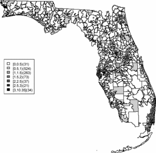
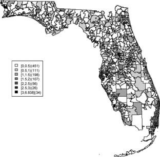
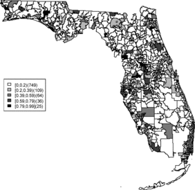
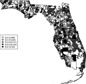
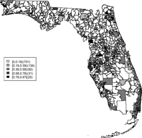
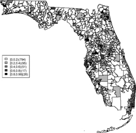
Relative risk estimates from both models are compared and exceedence probabilities are used as cluster diagnostics to investigate geographic patterns of possible clusters of the disease. In the SMR map, we can see aggregated risks in the middle of the state and some apparent hot spots scattered over the northeast and along the coasts. Figures 2 and 3 display the posterior mean relative risk estimates under the BYM model and the SPC model fitted to these data. While the overall variation of risk is similar to the SMR, the BYM and SPC produce smoother (shrunken) risk estimates. Additionally, the BYM model produces a smoother pattern of relative risks than the SPC model since it does not directly model the excess number of zero values.

Figure 2. The estimated relative risk from the BYM model at each zip code area.

Figure 3. The estimated relative risk from the SPC model at each zip code area.

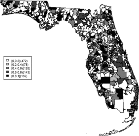
Rather than observing only risk estimates, another approach to cluster detection is using the posterior sampling output from a converged sampler providing an estimate of the exceedance probability of relative risk (Richardson et al. 2004; Lawson 2013). The maps of exceedance probability of the two models are displayed in Figures 4–7 with one and two as the threshold values. The cluster pattern seems to be similar to risk estimates. With higher thresholds, we see that fewer areas appear in excess. In fact, one concern about the exceedence probabilities is that they were designed to detect hot spot clusters. However, a group of high risks appears in the middle of the state using the exceedence probability which strongly suggests localized concentration. This contrasts with the isolated hot spots found in coastal areas (such as the South Beach area of Miami). Although the exceedence probability is the most commonly used example of posterior measures in cluster detection (Richardson et al. 2004), it can be sensitive to model specification (Lawson 2013, ch. 6). Another possibility is to use posterior measures based on exceedence probability of residuals.

Figure 4. The exceedance probability of relative risk greater than one from the BYM model.

Figure 5. The exceedance probability of relative risk greater than one from the SPC model.

Figure 6. The exceedance probability of relative risk greater than two from the BYM model.

Figure 7. The exceedance probability of relative risk greater than two from the SPC model.

Figures 8–11 display maps of exceedence probability of standardized residuals for both models with zero and one as the threshold values. The cluster patterns in the exceedence probability of residuals are slightly different than the one of relative risk but the group of zip code areas in the middle of the state still shows up with a high probability. There are some hot spots along the coasts, in the north–east and north–west parts of the state.

Figure 8. The exceedance probability of residual greater than zero from the BYM model.

Figure 9. The exceedance probability of residual greater than zero from the SPC model.

Figure 10. The exceedance probability of residual greater than one from the BYM model.

Figure 11. The exceedance probability of residual greater than one from the SPC.

Tables 2 and 3 display the zip codes with the highest and lowest relative risks of BYM and SPC models. Both models yield similar results. The highest and lowest relative risks appear in similar areas with a slightly different rank order of risk. There are 451 zip codes with no cases and the SPC estimates the relative risks less than 0.01 for 451 areas. This adds support to the view that that SPC model fits the data better than the BYM model.

5. DISCUSSION AND CONCLUSION

The aim of this project is to investigate spatial clusters of relative risk of the Florida childhood cancer. Two spatial Bayesian models, SPC and BYM, were applied, and DIC and WAIC suggest that the SPC model has a better performance in terms of goodness of fit. The MSPE suggests comparable predictive ability. Cluster diagnostics are summarized based on exceedence probability of relative risk and residual. In general, there are two common types of clustering: (1) a hot spot which is found in a single region and (2) a cluster which is found in a group of areas with unusual relative risk. Exceedence maps of SPC, both for relative risk and residuals, appear to have evidence of disease clustering in a number of relatively dispersed areas across the state especially in the north central Florida (i.e., Tavares) and hot spots along northwest (i.e., Panama city), southwest (i.e., Goodland), and southeast coasts (i.e., Fort Lauderdale). They also show some concentration of hot spots in the northeast region (i.e., Jacksonville). The results are consistent with the BYM model as well.

Our work can be compared to an investigation conducted earlier by Amin et al. (Amin et al. 2010). The spatial analysis using SaTScan suggested circular clusters in the southwest and north central Florida regions with a relatively bigger size. The shape of a scanning window will affect the resulting clusters found. The shape of the spatial pattern of a cluster is not predetermined in our Bayesian convolution models. SaTScan requires a circular or fixed shape of the cluster while the correlation structure in the convolution models allows for more flexibility in modeling disease variation and hence identifying clusters with different sizes and shapes. Moreover, SaTScan disregards whether the regions within the scanning window are neighbors or not. Hence, SaTScan is more likely to detect clusters with a larger size (Aamodt, Samuelsen, and Skrondal 2006). In addition, convolution models can also suggest smaller hot spots in various areas, such as in our study along the southeast coast, which were not detected using SaTScan in the earlier study. Our study did not include additional covariate adjustment in the models but did use expected rates adjusted for the population at risk. Note that, additionally, a Bayesian spatio-temporal analysis with a focus on cluster detection could be performed (see, e.g., Hossain and Lawson 2010 for examples) but we did not pursue this as the temporal variation appeared negligible (as noted in the earlier study).

REFERENCES

- Aamodt, G., Samuelsen, S.O., and Skrondal, A. (2006), “A Simulation Study of Three Methods for Detecting Disease Clusters,” International Journal of Health Geographics, 5, 15, doi:10.1186/1476-072X-5-15.
- Amin, R., Bohnert, A., Holmes, L., Rajasekaran, A., and Assanasen, C. (2010), “Epidemiologic Mapping of Florida Childhood Cancer Clusters,” Pediatric Blood & Cancer, 54, 511–518.
- Besag, J., York, J., and Mollié, A. (1991), “Bayesian Image Restoration, With Two Applications in Spatial Statistics,” Annals of the Institute of Statistical Mathematics, 43, 1–20.
- Best, N., Richardson, S., and Thomson, A. (2005), “A Comparison of Bayesian Spatial Models for Disease Mapping,” Statistical Methods in Medical Research, 14, 35–59.
- Brooks, S.P., and Gelman, A. (1998), “General Methods for Monitoring Convergence of Iterative Simulations,” Journal of Computational and Graphical Statistics, 7, 434–455.
- Celeux, G., Forbes, F., Robert, C.P., and Titterington, D.M. (2006), “Deviance Information Criteria for Missing Data Models,” Bayesian Analysis, 1, 651–673.
- Cheung, Y.B. (2002), “Zero-Inflated Models for Regression Analysis of Count Data: A Study of Growth and Development,” Statistics in Medicine, 21, 1461–1469.
- Gelfand, A.E., and Ghosh, S.K. (1998), “Model Choice: A Minimum Posterior Predictive Loss Approach,” Biometrika, 85, 1–11.
- Gelman, A. (2006), “Prior Distributions for Variance Parameters in Hierarchical Models’’ (comment on article by Browne and Draper), Bayesian Analysis, 1, 515–534.
- Gelman, A., Hwang, J., and Vehtari, A. (2013), “Understanding Predictive Information Criteria for Bayesian Models,” Statistics and Computing, 1–20.
- Ghosh, S.K., Mukhopadhyay, P., and Lu, J.-CJ. (2006), “Bayesian Analysis of Zero-Inflated Regression Models,” Journal of Statistical Planning and Inference, 136, 1360–1375.
- Hossain, M., and Lawson, A.B. (2006), “Cluster Detection Diagnostics for Small Area Health Data: With Reference to Evaluation of Local Likelihood Models,” Statistics in Medicine, 25, 771–786.
- ——— (2010), “Space-Time Bayesian Small Area Disease Risk Models: Development and Evaluation with a Focus on Cluster Detection,” Environmental and Ecological Statistics, 17, 73–95.
- Lawson, A.B. (2006), Statistical Methods in Spatial Epidemiology (2nd ed.), New York: Wiley.
- ——— (2013), Bayesian Disease Mapping: Hierarchical Modeling in Spatial Epidemiology (2nd ed.), Boca Raton, FL: CRC Press.
- ——— (2014), “Hierarchical modeling in spatial epidemiology,” WIREs Computational Statistics , 6, 405–417.
- Richardson, S., Thomson, A., Best, N., and Elliott, P. (2004), “Interpreting Posterior Relative Risk Estimates in Disease-Mapping Studies,” Environmental Health Perspectives, 112, 1016–1025.
- Rotejanaprasert, C. (2014), “Evaluation of Cluster Recovery for Small Area Relative Risk Models,” Statistical Methods in Medical Research, DOI: 10.1177/0962280214527382.
- Song, H.-R., Lawson, A., D’Agostino, Jr. R.B., and Liese, A.D. (2011), “Modeling Type 1 and Type 2 Diabetes Mellitus Incidence in Youth: An Application of Bayesian Hierarchical Regression for Sparse Small Area Data,” Spatial and Spatio-Temporal Epidemiology, 2, 23–33.
- Spiegelhalter, D.J., Best, N.G., Carlin, B.P., and Van Der Linde, A. (2002), “Bayesian Measures of Model Complexity and Fit,” Journal of the Royal Statistical Society, Series B, 64, 583–639.
- Watanabe, S. (2010), “Asymptotic Equivalence of Bayes Cross Validation and Widely Applicable Information Criterion in Singular Learning Theory,” The Journal of Machine Learning Research, 11, 3571–3594.