Analyzing 2000–2010 Childhood Age-Adjusted Cancer Rates in Florida: A Spatial Clustering Approach

Abstract

In this work, we apply a Bayesian hierarchical model that uses spatial clustering techniques to data from the Florida Association of Pediatric Tumor Programs (FAPTP) for the period 2000–2010. The goal is to determine whether there are statistically significant childhood cancer clusters at the Zip Code Tabulation Area (ZCTA) level of geography. The model provides estimates of the uncertainty associated with the clustering configurations, which is typically lacking in classical analyses of large datasets where a unique clustering representation can be insufficient. The model also allows covariate adjustment for known risk factors, bringing further relevant information, and it produces clusters that are spatially contiguous, enabling simple interpretation. The output clustering map is able to capture such patterns as the high-risk area that appear in the Southwest, Northeast, and Northwest Florida, which is consistent with the previous studies, but with finer details and deeper insight into year-specific features. New findings from the latest data, from 2008 to 2010, were also obtained and investigated. Our post-hoc validation of the clusters provides evidence for concluding that areas of elevated risk exist.

KEY WORDS::

• Bayesian hierarchical models
• Epidemiology
• Marginal likelihood
• Pediatric cancers
• Reversible jump MCMC

1. CHILDHOOD CANCER RATES IN FLORIDA

In the state of Florida, elevated rates of pediatric cancer in some regions have been previously reported (see Amin et al. 2010), which led us to investigate possible risk factors associated with such regions. Using data on pediatric cancer counts, together with additional demographic and geographic information available for Zip Code Tabulation Areas (ZCTAs) in the state of Florida from 2000 to 2010, we seek to identify regions that have higher risk of pediatric cancer in case further public health investigation should be performed to determine causal factors.

Before applying advanced statistical methods to identify ZCTAs with high risk, we first explore the dataset. To avoid possible confounding due to age, we calculate the age-adjusted rates using indirect standardization with the internal standard population (see, e.g., Curtin and Klein 1995). More specifically, let d_itj be the observed count of reported cases for site i, time t, and age group j, where i = 1, 2, …, N = 983 indicates the ZCTAs, t = 1, …, T = 11 corresponds to the year (2000 to 2010), and j = 1, …, J = 4 represents four age groups: [0, 4], [5, 9], [10, 14], and [15, 19]. We let p_itj be the corresponding population size, and calculate the crude rate for the standard population M_t = ∑_{i, j}d_itj/∑_{i, j}p_itj for each year t. The incidence rates for each age group were pooled across the entire state to serve as the standard m_tj (see, e.g., Kulldorff et al. 1997). The indirect age-adjusted rate R_it per 100, 000 population at site i and time t is calculated as and we investigate the log-transformed age-adjusted rate, Y_it = log (R_it). We add a reasonably small positive value to the calculated rates R_it that are 0, to avoid the logarithm of zero. Note if the adjustment is too small, it can potentially introduce extreme clusters, which can deter our goal to identify hot spots. We empirically choose 0.5 by comparing the raw and transformed data distributions, and it well preserve the patterns, in particular for the large observations, without introducing a cluster of small values. Other choices such as 0.1 lead to similar patterns of data distribution, and conclusions of hot spots.

The age-adjusted cancer rates can also be calculated by choosing m_tj = ∑_id_itj/∑_ip_itj as the age-specific rates for indirect standardization, or using direct standardization as the exact formula provided by the Surveillance, Epidemiology, and End Results (SEER) program (seer.cancer.gov) of the U.S. National Cancer Institute (NCI) (2010). However, both calculations introduce a larger discrepancy between zero and nonzero rates that is more sensitive to the small-amount adjustment for the log-transformation, and hence carry an extra burden of modeling the zero inflation. Other normalization and variance stabilization techniques such as Freeman–Tukey transformation (see, e.g., Cressie and Chan 1989) can also be considered. In previous studies, such as Amin et al. (2010), it is also common to calculate the cancer rates adjusted not only for age, but also for gender and race information. Alternatively, we explicitly explore the effects of sex and race by considering both the factors as covariates in a regression model for the Y_it. This allows us to further explore the potential regional heterogeneity in these effects, so that we can cluster the regions based on not only the mean level of Y_it, but also the regional effects of the covariates. In this study, we consider the percentage of white residents X_it1 and the percentage of male residents X_it2 at each ZCTA i = 1, 2, …, N and each year t = 1, 2, …, T as covariates.

Figure 1 shows the log-transformed age-adjusted pediatric cancer rates, Y_it, of the N = 983 ZCTAs in Florida over the T = 11 years in (a), and the map of the ZCTAs in (b), with 13 ZCTAs highlighted that correspond to the upper 0.13% extreme observations of all Y_it’s. The threshold 0.13% is empirically chosen by investigating the histogram as our initial exploration of high-risk areas. We note that the data are unevenly distributed, particularly in Southern Florida. Densely clustered ZCTAs are seen on the east and west coast of South Florida, while the ZCTAs in the middle are less dense, with larger areas but possibly smaller population compared to the urbanized coasts.

Figure 1. Visualization of the (a) calculated log-transformed age-adjusted caner rates with upper 0.13% extreme observations, and (b) 983 ZCTAs in the map of Florida with a few highlighted areas that correspond to ZCTAs in the left panel.

From our preliminary exploration in Figure 1, it is plausible that the potential hot spots with high risk tend to appear in different regions and years. For instance, the three highest peaks in Figure 1(a) correspond to ZCTA 34101 from the Southwest Florida in 2000, ZCTA 34445 from the Northeast Florida in 2007, and ZCTA 32530 from the Northwest Florida in 2009, respectively. However, for the remaining years, these areas have relatively smaller log-rates. Such areas may appear as transient hot spots, and a clustering method with temporal smoothing can mask such patterns and result in estimates that are over-smoothed due to the regression-toward-the-mean phenomenon. On the other hand, the local similarity is remarkable. For instance, there is a group of ZCTAs that have extreme observations of the log-rates in Northeast Florida, particularly for 2005, and it is of interest to identify groups of ZCTAs with elevated risk and geographic proximity, rather than identifying a single ZCTA that has extreme values that may be due to chance. It is also reasonable to assume that adjacent ZCTAs share similar childhood cancer risk due to their similar environmental and socio-economic conditions. After the investigation, we conduct a year-by-year analysis to identify spatial clusters with similar levels of cancer risk, and shall suppress Y_it into Y_i in the following sections for model description. Furthermore, cancer rates are associated with demographic variables such as gender and race, so our analysis includes that information.

2. SPATIAL CLUSTERING MODEL

2.1 Literature Review

The Bayesian approaches for randomly partitioning the study region and searching nonoverlapping, spatially contiguous clusters, have been widely recognized and fully developed with applications in disease mapping and risk assessment. Popular choices in the literature are using Voronoi Tessellations (see, e.g., Knorr-Held and Raßer 2000; Kim, Mallick, and Holmes 2005; Feng et al. in press), or Bayesian Treed Partitions (see, e.g., Gramacy and Lee 2008; Konomi, Sang, and Mallick 2014). The latter choice commonly provides regularly shaped clusters such as rectangles or bands such as in the examples of Gramacy and Lee (2008) and Konomi, Sang, and Mallick (2014), unless ad hoc splitting rules are specified for the treed partition or the study domain is topologically transformed. The tessellation approach, however, can provide more generally shaped polygons, which better describe the disease maps, and it further allows the flexibility of choosing certain distance measures that are suitable for the study domain. We therefore consider the tessellation approach for searching regions with high risk of disease in the following context.

Our response variable is the log-rate Y_i and our model includes an intercept and two covariates, percentage of male residents, and percentage of white residents, for the i = 1, 2, …, N ZCTAs in Florida. A spatial clustering configuration ϖ = (d, G_d) under tessellation approach is defined by two components: d is the number of clusters, and G_d = {g₁, …, g_d} are the d cluster centers, which is a subset of the N sites that determine the cluster membership of all sites according to the minimal distance criterion. That is, the clustering label of the ith site is assigned to k if the kth cluster center g_k is the first center in G_d that has the smallest distance from the site i.

It is evident that such spatial clustering configurations can strongly depend on the selection of distance between sites. We choose the ordinary Euclidean distance based on the spatial coordinates of the centroids of ZCTAs, which typically does not result in tied distances. Other geo-spatial distances can be also considered when the adjacency information of each ZCTA, represented as polygons for areal data, is available. Note that the number of clusters d is bounded above when we specify a minimal cluster size to ensure stable estimates of coefficients for the regressors.

2.2 Model Description

To identify spatial clusters of the data, we consider a hierarchical model. First, we place a prior distribution on the clustering configuration, π(ϖ). Given the clustering configuration ϖ with d clusters, C₁, …, C_d, the covariate X_i affects the response Y_i differently for each cluster. More specifically, we have where we assume the sites within the same cluster share both the regression parameters β_r and the variation σ²_r, which are both varying across clusters. In the model specification above, λ_k is an overall signal-to-noise ratio, or detectability for the kth effect β^k_r for all r = 1, 2, …, d. We update this scaling parameter by assuming the conjugate inverse Gamma prior with shape a_λ and scale b_λ, chosen such that the specified density is rather dispersed to allow the estimate of λ to be more data driven. One common choice is a_λ = 2 and b_λ = 0.01 to achieve this. We similarly choose a_σ and b_σ to yield a dispersed prior density for the cluster-specific variation σ²_r.

Let be the collection of all possible clustering configurations ϖ. For the distribution of a spatial clustering configuration on , we consider the prior model π(ϖ) = π(Gd | d)π(d | κ)π(κ), with π(d | κ)∝(1 − κ)d − 1 for d = 1, …, N0 and κ ∈ (0, 1). N0 is the upper bound of d, which is less than or equal to N. Here, the hyperparameter κ controls the penalty of model complexity introduced by a large d. The prior for d is a power decay law under this elicitation, since when κ is larger, d is more likely to be small, while when it is fixed at a tiny value, d is almost uniformly distributed over {1, 2, …, N0}, indicating weak prior information. Inspired by the more traditional approach for model selection, we reparameterize κ as an exponential decay: π(d | κ)∝exp ( − tan (πκ/2)d) for κ ∈ (0, 1). For instance, when tan (πκ/2) is fixed to be , it is closely related to the well-known Akaike information criterion (AIC) if α0 = 2, or Bayesian information criterion (BIC) if α0 = log (N). It is evident that the value of κ can affect the posterior behavior of the number of clusters d. We therefore obtain the posterior estimate of κ from the data by eliciting another hierarchy π(κ) = Uniform(0, 1) that is flat over its support when no prior information is available, otherwise one can specify a general Beta density prior on (0, 1) to incorporate any prior belief on d. Note that since d is bounded above by N0, it requires ∑N0d = 1π(d | κ) = 1, which yields (1) where f(κ) = exp ( − tan (πκ/2)). Next, conditional on d, we also consider the uniform prior for centers π(Gd | d) = (N − d)!/N! where the possible Gd’s receive equal probability of being the cluster centers.

The full details of the model likelihood are described in Appendix A, and the implementation via the Markov chain Monte Carlo (MCMC) technique is described in Appendix B, where we embed the reversible jump MCMC (Green 1995) algorithm into Gibbs sampling scheme, for stochastically searching clustering configuration ϖ based on its integrated likelihood, with β_r’s and σ²_r’s proposed from their full conditional densities and hence marginalized out, that is, we restrict our attention on model search by spontaneously proposing the data-driven parameters. This is a different approach from Knorr-Held and Raßer (2000) and Feng et al. (in press) with extra efforts on tailoring the full likelihood to different proposal densities for the parameters during the model search.

The proposed clustering model is similar to the one proposed by Kim, Mallick, and Holmes (2005), which also uses Voronoi tessellations and piecewise Gaussian processes. However, there are several notable differences. First, our approach does not involve modeling the spatial dependence within each cluster under ϖ, for two main reasons: (i) Certain ZCTA can have extremely high risk of disease, which largely exceeds that of the surrounding ZCTAs, and hence forms a singleton cluster. The spatial dependence within such singleton clusters is not quite meaningful and can cause unstable estimates. The spatial smoothing effects can be prone to clusters with more member ZCTAs rather than singleton clusters, which however may manifest the disease patterns and (ii) While Appendix A shows the marginal likelihood after integrating β_r’s and σ²_r’s out has a convenient form, the marginal model likelihood that further integrates the spatial parameters out is known to be intractable, and is numerically evaluated in Kim, Mallick, and Holmes (2005). Consequently, the computation cost aggregates over the MCMC iterations, which requires a large number of total runs for searching ϖ’s in a massive candidate set particularly for large N.

Second, we allow the adaptive learning of the overall effects of covariates by assuming random λ_k’s that are updated through MCMC iterations. We further allow the adaptive learning of the penalty on the number of clusters from the data by sampling κ. Empirical results suggest the adaptive learning processes can potentially improve the mixing comparing to the choice by Kim, Mallick, and Holmes (2005), and the posterior behaviors of λ_k’s and κ are closely related to the number of clusters and can manifest the complexity of the data structure. With diffuse prior on λ_k’s and κ, we seek for data-driven penalties for model complexity, which is relevant as the introduction of extra clusters and hence more β^k_r’s can easily yield better model fit particularly when the within-cluster correlation is intendedly dropped.

Third, we explicitly update β_r’s and σ²_r’s, which are not nuisance parameters in this study, with an extra Gibbs step to draw their posterior samples based on which our proposed post hoc procedure is executed for identifying hot spots.

Finally, as described in Appendix C, we employ a model averaging procedure proposed in Dass et al. (in press) to obtain a central clustering configuration from the full posterior samples of ϖ, which produces clusters with more general shapes comparing to the commonly used posterior modal sample . See Appendix C for more detailed discussions.

3. SPATIAL CLUSTERING OF CHILDHOOD CANCER RATES IN FLORIDA

We fit the spatial clustering model to the age-adjusted childhood cancer log-rates in Florida for each of the 11 years, with the regression parameters that change between different clusters. The summary of posterior distribution of the number of clusters d with the posterior modal estimates for each year is shown in Table 1, while the summary of model parameters for measuring the uncertainty of clustering information and data complexity is given in Appendix C. It is seen that the estimated number of clusters and configurations are quite distinct across years, which further justifies this year-by-year study.

Table 1. Posterior distributions and estimates of the number of clusters d for the 11 years

d	2000	2001	2002	2003	2004	2005	2006	2007	2008	2009	2010
3				0.246
4				0.349			0.007
5				0.347			0.298
6				0.059	0.057		0.167			0.323
7					0.055		0.487			0.417
8					0.197		0.038			0.257
9	0.225				0.171		0.003	0.231		0.003
10	0.517		0.161		0.267			0.521	0.004		0.219
11	0.251		0.118		0.199	0.037		0.122	0.063		0.595
12	0.006	0.193	0.477		0.048	0.194		0.113	0.161		0.171
13		0.514	0.184		0.006	0.386		0.013	0.533		0.014
14		0.229	0.050			0.309			0.194		0.001
15		0.055	0.011			0.073			0.044
16		0.007				0.001			0.001
17		0.002
	10	13	12	4	10	13	7	10	13	7	11

NOTE: A bold number indicates the highest posterior probability.

For each year, we extract the central clustering configuration , which integrates the clustering information over b = 1, 2, …, B posterior samples. The detailed description of the procedure is given in Appendix C. For each cluster and posterior sample b, we estimate the cluster mean age-adjusted log-rates by averaging the predicted values over member sites , where denotes the regression parameter value assigned to site i, as determined by its membership in ϖ^(b) in the bth posterior sample. We then obtain the labels of each cluster by sorting the posterior mean in descending order. Consequently, a cluster with a smaller label is considered to be more risky in terms of pediatric cancer. 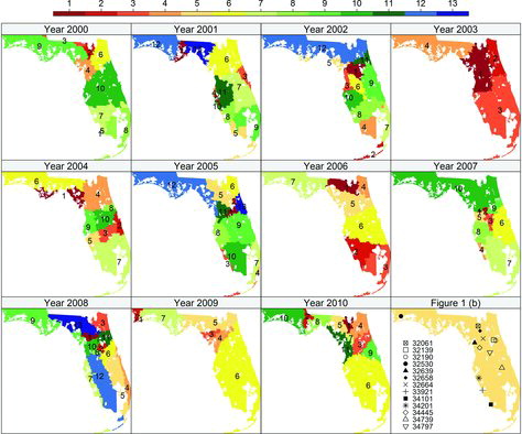We calculate the posterior mean with 95% credible interval for the cluster means of age-adjusted rates, using the back-transformed posterior samples ’s, and plot them versus the cluster labels in Figure 2, with different scales for the y-axis for each year. The posterior mean can be viewed as the estimated number of cases per 100, 000 children for each cluster under the way of calculating age-adjusted rates in Section 1. We also plot the map of the extracted central configuration with cluster labels, which is shown in Figure 3, for all 11 years. We also show the several high-risk ZCTAs from Figure 1, the preliminary investigation, in the last panel of Figure 3 for comparisons. Note that the cluster labels and colors are consistent for both Figure 2 and 3, such that one can match the estimated cluster mean with the spatial locations.

Figure 2. Posterior mean and 95% credible interval of the cluster mean age-adjusted rates (y-axis) versus cluster labels r = 1, 2, …, d (x-axis) for the 11 years.

Figure 3. Map of the central clustering configuration with clustering labels assigned by descending order of the posterior mean of the cluster mean estimates for the 11 years.

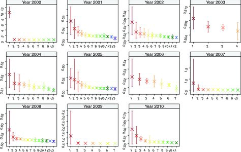
To further identify potential hot spots out of the high-risk clusters in each year, we compare the estimated cluster mean of the cluster versus its surrounding clusters, as shown in Figure 3. Note that the choice of Euclidean distance between the coordinates of centroids for the spatial clustering model tend to yield convex, sphere-shaped clusters. Consequently, a concave cluster could be represented by several convex clusters arranged in a concave shape, and this would need joint investigation. Therefore, we define the probability of being a hot spot (poh) for a set of central clusters , based on the its neighbor set that is comprised of all surrounding clusters with labels larger than that of the members in , to be (2) Clusters with a high value of can potentially be the hot spots for further investigation. Based on this criterion and the spatial information from Figure 3, we scan potential hot spots from the spatial clustering model for each year as follows:

1. In 2000, the high-risk ZCTA 34101 from Southwest Florida, as shown in Figure 1(a), forms a singleton cluster with the highest risk of the pediatric cancer and . Figure 2 indicates it has much higher log-rates than the remaining clusters. The other high-risk cluster is centered on ZCTA 32658 in North Florida, as shown in Figure 1(a), with a total of 12 member ZCTAs and . Moreover, we notice that cluster 3 is considered as a surrounding cluster for calculating from Figure 3. By combining the two high-risk clusters, we have , which is even lager. Hence, there is a strong evidence of a hot spot in year 2000 that consists of both cluster 2 and 3 in North Florida. The remaining sets of clusters have poh values dramatically dropped. For instance, cluster 4 also has higher risk, however when compared to the surrounding clusters {6, 9, 10} with larger cluster labels.

2. In 2001, cluster 1 in Northwest Florida around ZCTA 32334 is detected as a highly potential hot spot with . Another potential hot spot in West Florida consists of both cluster 2, which is centering around the high-risk ZCTA 34201, and cluster 4 around ZCTA 33763, with for the joint set. Note that cluster 2 itself is less qualified as a hot spot, with a smaller , even though ZCTA 34201 has higher risk. This example suggests that the observations of certain high-risk areas can be smoothed by that of surrounding areas with moderately high risk.

3. In 2002, cluster 1 consists of 45 ZCTAs in North Florida including the three high-risk ZCTAs 32639, 32139, and 34797 in Figure 1(a). It can be potentially identified as a hot spot with a high . The remaining sets of clusters have relatively smaller values of poh.

4. In 2003, the cancer risk is overall lower than in the remaining years. ZCTAs in cluster 1 that center around ZCTA 34442, as shown in Figure 3, have higher risk than the remaining areas, with the largest in that year.

5. In 2004, the cluster with highest risk has and it consists of 21 member ZCTAs. The high-risk ZCTA 34739 from the preliminary scan is contained in cluster 3, with .

6. In 2005, cluster 1 with 17 ZCTAs around the high-risk ZCTA 32190, and cluster 2 with 7 ZCTAs around ZCTA 32181, form a hot spot near north central Florida with . Cluster 3 along the west coast of South Florida, which includes the high-risk ZCTA 33921, has , while cluster 4 along the east coast of South Florida with 44 ZCTAs around ZCTA 33128, has .

7. In 2006, the regions in Southern Florida represented by combining clusters 2 and 3 have significantly higher risk than the Central Florida region represented by cluster 6, with . This is consistent with the findings by Amin et al. (2010). We also find the Northern Florida area represented by clusters 1 and 4 with relatively high value of .

8. In 2007, cluster 1, consisting of 4 ZCTAs around the high-risk ZCTA 34445 from the initial scan, can be potentially identified as a hot spot with a high . Cluster 4, near the west coast of South Florida around ZCTA 34224, forms another potential hot spot with .

9. In 2008, cluster 1 in North Central Florida, containing 10 ZCTAs around the high-risk ZCTA 32664 in Figure 1(a), has a large potential of being a hot spot with . Another hot spot, cluster 3 at the northeast corner around ZCTA 32207, has high . In Southern Florida, the east and west coast areas represented by cluster 4 and 7 have higher risk than the central regions represented by cluster 5 and 12, with and , respectively.

10. In 2009, cluster 1 in Northwest Florida, consisting of adjacent ZCTAs around the high-risk ZCTA 32530 in Figure 1(a), can be potentially identified as a hot spot with . Cluster 2 also has a relatively high value with . Another potential hot spot that is comprised of cluster 3 and 4 around the west coast of North Central Florida has .

11. In 2010, the three clusters with the highest risks can be all identified as hot spots in Northern Florida with relatively large , , and . The high-risk ZCAT 32061 from initial analysis belongs to cluster 1, which contains 10 ZCTAs in North Florida.

Finally, by jointly investigating the distributions of hot spots and clustering label assignment according to risks from 2000 to 2010 in Figure 3, we conclude that, overall, the hot spots and high-risk clusters are more likely to be observed in North Florida than in South Florida. In particular, we have recognized hot spots and the high-risk clusters around North Florida and North Central Florida for the years 2000, 2002, 2003, 2005, 2006, 2007, 2008, and 2010. In South Florida, the coastal areas have generally higher risk than the inland regions, and the gap is particularly visible for year 2005 and 2008.

4. CONCLUSION

We have applied a Bayesian hierarchical model that uses a spatial clustering method to the age-adjusted childhood cancer rates in Florida from 2000 to 2010. The model is able to capture clustering and identify high-risk regions. The Bayesian estimates provide further insight into the uncertainty associated with the clustering configuration suggested by this dataset, and give statistical validation of high-risk clusters. Our main findings are consistent with the previous study in Amin et al. (2010), which had a study period from 2000 to 2007 and concluded that there were two major clusters: the Southern Florida cluster (2006–2007) and the North Central Florida cluster (2001–2004), based on scan statistics. Nevertheless, our cluster analysis and post hoc validation by different years produce more detailed maps. For instance, the centroids of the North Central Florida clusters switch from different regions in North Central Florida over time in Figure 3. Also, in year 2007, we found the west coast areas (cluster 4) form a hot spot and have significantly higher risk compared to the other regions in the Southern Florida (cluster 7). Our approach also captures the clustering pattern for the new data from 2008 to 2010, which are consistent with the exploratory data analysis. All extreme values have entered the high-risk clusters, which are recognized as highly potential hot spots. In our study, the regional covariates effects for race and gender turn out to be nonsignificant on the log-transformed age-adjusted rates.

APPENDIX A: FULL DESCRIPTION OF THE MODEL LIKELIHOOD

From the data perspective, we write the model likelihood at the cluster level by grouping the sites in each cluster, that is, and for the rth cluster with n_r member sites, as follows: (A.1) When clustering is of primary interest, we integrate out the nuisance parameters β_r with the prior , so the likelihood (A.1(A.1) ) becomes (A.2) where Λ = diag_{1 ⩽ k ⩽ p}λ_k, and a larger variance is introduced in (A.2(A.2) ) compared to (A.1(A.1) ). We then integrate out the nuisance parameters σ²_r from (A.2(A.2) ) with the prior , so the likelihood becomes (A.3) where denotes a multivariate Student’s-T distribution with location vector μ, scale matrix Σ, and degrees of freedom ν. It is immediately seen that the marginal likelihood for ϖ given the data and λ_k’s depends on the hyperparameters a_σ and b_σ. Comparing (A.3(A.3) ) to (A.2(A.2) ), we note that is an estimator of σ²_r that is between the prior mode and prior mean for the inverse Gamma density we specify, and it is well known that the multivariate Student’s T distribution generally involves more uncertainty than the multivariate Normal density with the same parameters. Our empirical results suggest that the posterior behavior of the clustering configurations are robust across several reasonable choices of a_σ and b_σ, in particular when the λ_k’s (and hence Λ) are updated throughout the MCMC iterations. Alternatively one can choose the noninformative Jeffery’s prior by setting a_σ = b_σ = 0, so the marginal likelihood (A.3(A.3) ) for is no longer multivariate Student’s-T distributed, but rather proportional to (A.4) In this application, we stick to the common choice of hyperparameters a_σ and b_σ that define a rather dispersed prior density for σ²_r, while we note the flexibility of eliciting different hyperparameters, such as consistent estimates from data with no clusters, or the noninformative priors.

From (A.3(A.3) ) it is immediately seen that for fixed and κ, the posterior propriety holds, that is, let , , and , giving (A.5) based on the fact that is a finite set. It follows that the propriety for the full posterior distributions of also holds since we specified the conjugate prior for and the uniform prior for κ.

APPENDIX B: IMPLEMENTATION OF THE SPATIAL CLUSTERING MODEL

To fit the spatial clustering model, the set of parameters are estimated under the Bayesian framework. Since our prior choices for the mean and scaling parameters are conjugate, we consider the Gibbs sampler by deriving the full conditional distributions. On the other hand, since the cardinality of the set for ϖ can be quite large due to large N, and updating ϖ involves interchanging variable model dimensions, we shall adopt an embedded reversible jump MCMC algorithm of Green (1995) for updating ϖ at each Gibbs cycle that consists of following steps:

1. Update ϖ: In this step, we consider updating the clustering configuration ϖ = (d, G_d), which determines the dimensionality of the parameters conditional on the remaining parameters and κ. For notation simplicity, we suppress and κ in the conditioning part of all probability densities below. We construct the reversible jump MCMC step for updating the triplet with potentially changing dimensions. From the current clustering configuration ϖ with associated parameters , suppose we propose a new configuration ϖ* with associated parameters , we define an auxiliary and let . The corresponding invertible map to is one-to-one with the Jacobian to be unity. We first propose ϖ* from a certain probability mass function H( · ) given the current clustering configuration ϖ, then propose for a certain proposal density function h( · ). Consequently, the Metropolis–Hasting ratio for accepting the proposed triplet is (B.1) We choose the proposal density to be the posterior density, that is, . More specifically, for r = 1, 2, …, d, we first sample each σ*_r from (B.2) which is an inverse Gamma density with shape parameter a_σ + n_r/2 and scale parameter with . Next, we sample β*_r based on σ²*_r: (B.3) Under this choice of proposal density function h( · ), we can substitute with from (A.5(A.5) ). Therefore, the acceptance ratio in (B.1(B.1) ) becomes (B.4) Using the fact that the ratio (B.4(B.4) ) reduces to (B.5) When both the prior and proposal density of ϖ are diffuse, for instance, under tiny values of κ and uniform proposal density H( · ), the acceptance ratio in (B.5(B.5) ) is mainly determined by the marginal likelihood ratio with (B.6) which is a product of the multivariate Student’s-T densities under (A.3(A.3) ), or more specifically (B.7) where .

Next, we consider specifying the probability mass function H( · ) for proposing ϖ*, which involves constructing plausible move types that give higher chance of exploring the set of clustering configurations that resemble the current ϖ in , potentially with different dimensions, that is, varying numbers of clusters d. The efficiency of implementing the reversible jump MCMC algorithm can heavily rely on searching such neighborhoods of ϖ in the full set .

To propose a new clustering configuration ϖ*, we consider one of the three steps: a Growth step that creates one more clusters, a Merge step that deletes an existing cluster, and a Shift step with the same number of clusters but different cluster centers, with prescribed proposal probabilities P(Growth) = P(Merge) = 0.4 and P(Shift) = 0.2 at each iteration, similar to the choice in Knorr-Held and Raßer (2000). The motivation underlying the choice of the prescribed probabilities, which gives higher chance of proposing a new clustering configuration with a different number of clusters d, is to fully explore the uncertainty associated with d. Next, to keep this article self-contained, we give the details of the three move types with the respective acceptance probabilities under our choice of the prior densities and proposal density h( · ), as follows:

1. Growth step (d, G_d) → (d + 1, G*_{d + 1}): We create a new cluster. We first draw a random variable uniformly distributed on the n − d noncenter sites, to determine the new cluster C* with center g*. Second, we draw another random variable r uniformly distributed on {1, …, d + 1} to determine the position of g* in G*_{d + 1}. The n*_r sites that have minimal distance from g* then automatically enter C*. In this case, and the acceptance rate is .

2. Merge step (d + 1, G_{d + 1}) → (d, G*_d): We delete one existing cluster and merge its members into other existing clusters. First, generate a random variable r that is uniformly distributed on {1, …, d + 1}, which determines the cluster C_r with center g_r to be removed, with all its members merging into one of the remaining clusters by the minimal distance criterion. The acceptance is the reciprocal of that in growth step.

3. Shift step: (d, G_d) → (d, G*_d): We adopt a shift step for moving a cluster center to one of its noncenter neighbors to potentially improve the mixing performance of the MCMC. For each location s, we define its K nearest locations in distance as its neighbors. Among d current cluster centers there are n(G_d) cluster centers that have at least one noncenter neighbors. Draw r ∼ Uniform{1, …, n(G_d)} to obtain one such cluster center g_r with m(g_r) noncenter neighbors. Second, draw l from {1, …, m(g_r)} uniformly. The lth noncenter neighbor becomes the new cluster center g*_r that replaces g_r in G_d. The acceptance probability is . We empirically choose K = 5 for this application, which results in reasonable acceptance rates.

2. Update : In this step, we consider sequentially updating and given the remaining parameters including ϖ, to guarantee newly sampled values for even when the proposed ϖ* with is not accepted in the preceding step, to potentially improve the mixing. Specifically, for each cluster r = 1, …, d, we sample β_r from (B.3(B.3) ), and then sample σ²_r from its full conditional density given β_r also, which is an inverse Gamma density with shape parameter a_σ + n_r/2 and scale parameter .

3. Update : In this step, we consider sequentially updating and κ given the remaining parameters. We sample λ_k from the inverse Gamma density with shape parameter a_λ + d/2 and scale parameter b_λ + ∑^d_{r = 1}(β^k_r/σ_r)²/2. Finally, we sample κ from , which is proportional to the prior density (1(1) ) under the uniform prior choice for κ. One can use the inverse cumulative density function (CDF) method by numerically approximating the CDF of (1(1) ).

APPENDIX C: POSTERIOR ANALYSIS OF THE SPATIAL CLUSTERING MODEL

To get posterior samples, we run three MCMC chains with different initial numbers of clusters and hence different starting values for the remaining parameters. For each chain, we run the model for 100, 000 iterations, which take around 30 min to complete on a 2.66 GHz Oct-core Intel Xeon E7-8837 processor. The convergence is concluded after 50, 000 iterations by monitoring the full and marginal likelihoods, and parameters at the site level. We then draw a posterior sample at every 100th iteration for each chain to reduce the autocorrelations of samples and repetitions of clustering configurations. We have a total of 1500 MCMC samples for inference. The posterior mean and 95% credible intervals for the scaling parameters λ_k for β^k_r’s and penalty parameter κ for number of clusters d are shown in Table 2. The posterior estimates of λ_k for the covariates percentage of male residents and percentage of white residents are relatively small comparing to that for the intercept. This indicates that the covariates effects are not far from zero with the adaptive scales. Comparing to the posterior probabilities of d in Table 1, a larger value for the data-driven estimates of κ indicates larger penalty, and generally yields smaller d.

Table 2. Posterior mean (2.5%, 97.5%th quantile) of the scaling parameter λ_k for k = 1 (intercept), k = 2 (percentage of male population), k = 3 (percentage of white population), and κ

	2000	2001	2002	2003	2004	2005	2006	2007	2008	2009	2010
λ1	785.9	210.2	228.0	431.9	230.9	242.2	157.4	299.4	234.2	508.5	284.2
	(357.4,	(101.8,	(108.2,	(131.1,	(97.0,	(123.4,	(60.5,	(136.8,	(110.3,	(205.8,	(131.1,
	1760.2)	439.8)	486.7)	1200.6)	501.6)	474.9)	373.8)	664.9)	469.5)	1179.1)	599.1)
λ2	0.010	0.011	0.009	0.009	0.009	0.009	0.010	0.010	0.010	0.009	0.011
	(0.002,	(0.002,	(0.002,	(0.002,	(0.002,	(0.002,	(0.002,	(0.002,	(0.002,	(0.002,	(0.002,
	0.041)	0.040)	0.036)	0.039)	0.040)	0.036)	0.041)	0.039)	0.043)	0.042)	0.041)
λ3	0.008	0.009	0.009	0.008	0.011	0.008	0.010	0.009	0.009	0.009	0.011
	(0.002,	(0.002,	(0.002,	(0.002,	(0.002,	(0.002,	(0.002,	(0.002,	(0.002,	(0.002,	(0.002,
	0.031)	0.037)	0.036)	0.033)	0.051)	0.030)	0.039)	0.036)	0.035)	0.038)	0.040)
κ	0.127	0.097	0.102	0.261	0.130	0.096	0.189	0.129	0.096	0.174	0.112
	(0.015,	(0.011,	(0.013,	(0.039,	(0.016,	(0.012,	(0.025,	(0.016,	(0.012,	(0.022,	(0.013,
	0.336)	0.262)	0.278)	0.614)	0.345)	0.266)	0.470)	0.350)	0.264)	0.424)	0.307)

We extract a central clustering configuration from the samples ϖ^(b) for b = 1, 2, …, B using the model-averaging procedure proposed in Dass et al. (in press). More specifically, we define the distance D measure between a pair of ZCTAs i and j as where I^(b)(i, j) is an indicator function of the event that area i and j are in the same cluster under the bth clustering configuration ϖ^(b). We then use a traditional hierarchical clustering procedure to obtain the central clustering configuration based on the distance measure D and the posterior mode of the number of clusters. Comparing to the posterior modal sample of ϖ, which is commonly used for summarizing clusters (see, e.g., Kim, Mallick, and Holmes 2005; Gramacy and Lee 2008), is not restricted to be a Voronoi tessellation, rather it involves clusters with more general shapes by integrating the clustering information over all posterior samples of ϖ. On the other hand, the posterior inference conditioning on can involve only partial information from the full posterior samples, while discarding considerable samples of ϖ^(b)’s that are similar to as its neighbor states in the model space . This can potentially lead to biased results in particular when the posterior probability mass on is low (for instance, around 0.1 for year 2000 in our analysis). Moreover, is restricted to a Voronoi tessellation with less flexibility and capability of summarizing the high-risk disease maps than . One can further evaluate the dispersion of the posterior samples of ϖ by comparing ϖ^(b)’s with using the agreement measures in Dass et al. (in press), and investigate the representativeness of for ϖ^(b)’s, which is high in this study. We further obtain the 95% credible intervals from cluster-wise estimated covariates effects by averaging over all member sites under for posterior sample b = 1, 2, …, B. The intervals for percentage of male residents and percentage of white residents span zero for all clusters, indicating the covariates effects are nonsignificant as manifested by posterior estimates of scales λ_k’s for k = 2, 3 which are relatively close to 0 comparing λ₁, posing less data evidence or high penalty for nonzero β^k_r’s.

References

- Amin, R., Rohnert, A., Holmes, L., Rajasekaran, A., Assanasen, C. (2010), Epidemiologic Mapping of Florida Childhood Cancer Clusters, Pediatric Blood Cancer, 54, 511–518.
- Cressie, N., Chan, N.H. (1989), Spatial Modeling of Regional Variables, Journal of the American Statistical Association, 84, 393–401.
- Curtin, L.R., Klein, R.J. (1995), Direct Standardization (Age-Adjusted Death Rates), National Center for Health Statistics Health People Statistical Notes, 6.
- Dass, S.C., Lim, C., Maiti, T., Zhang, Z. (in press), Clustering Curves Based on Change Point Analysis: A Nonparametric Bayesian Approach, Statistica Sinica. DOI: 10.5705/ss.2012.308.
- Feng, W., Lim, C., Maiti, T., Zhang, Z. (in press), Spatial Regression and Estimation of Disease Risks: A Clustering Based Approach,” Technical Report, Department of Statistics and Probability, Michigan State University.
- Gramacy, R.B., Lee, H. K.H. (2008), Bayesian Treed Gaussian Process Models With an Application to Computer Modeling, Journal of the American Statistical Association, 103, 1119–1130.
- Green, P.J. (1995), Reversible Jump Markov Chain Monte Carlo Computation and Bayesian Model Determination, Biometrika, 82, 711–732.
- Kim, H., Mallick, B.K., Holmes, C.C. (2005), Analyzing Nonstationary Spatial Data Using Piecewise Gaussian Processes, Journal of the American Statistical Association, 100, 653–668.
- Knorr-Held, L., Raßer, G. (2000), Bayesian Detection of Clusters and Discontinuities in Disease Maps, Biometrics, 56, 13–21.
- Konomi, B.A., Sang, H., Mallick, B.K. (2014), Adaptive Bayesian Nonstationary Modeling for Large Spatial Datasets Using Covariance Approximations, Journal of Computational and Graphical Statistics, 23, 802–829.
- Kulldorff, M., Feuer, E.J., Miller, B.A., Freedman, L.S. (1997), Breast Cancer Clusters in the Northeast United States: A Geographical Analysis, American Journal of Epidemiology, 146, 161–170.
- Surveillance, Epidemiology, and End Results (SEER) Program (www.seer.cancer.gov) SEER*Stat Database, “Mortality—All COD, Aggregated With State, Total U.S. (1969–2007) <Katrina/Rita Population Adjustment>”, National Cancer Institute, DCCPS, Surveillance Research Program, Cancer Statistics Branch, released June 2010. Underlying mortality data provided by NCHS (www.cdc.gov/nchs).