Who Is My Neighbor? The Spatial Efficiency of Partisanship

Abstract

Relative to its overall statewide support, the Republican Party has been over-represented in congressional delegations and state legislatures over the last decade in a number of US states. A challenge is to determine the extent to which this can be explained by intentional gerrymandering as opposed to an underlying inefficient distribution of Democrats in cities. We explain the “spatial inefficiency” of support for Democrats, and demonstrate that it varies substantially both across states and also across legislative chambers within states. We introduce a simple method for measuring this inefficiency by assessing the partisanship of the nearest neighbors of each voter in each US state. Our measure of spatial efficiency helps explain cross-state patterns in legislative representation, and allows us to verify that political geography contributes substantially to inequalities in political representation. At the same time, however, we also show that even after controlling for spatial efficiency, partisan control of the redistricting process has had a substantial impact on the parties’ seat shares. Supplementary materials for this article are available online.

KEYWORDS:

• Gerrymandering
• Spatial analysis
• Spatial efficiency

1 Introduction

From 2000 to 2016, summing over all statewide elections for the US Senate and all presidential contests, Republican candidates have received less than 48% of all votes cast. Yet during that same time period, they have received more than 52% of all seats contested in US congressional elections, 55% of all state lower chamber seats, and 56% of all seats in state upper chambers.

There are two related explanations for this underrepresentation of Democrats in legislatures. The first is partisan gerrymandering—the construction of electoral district boundaries to advantage one party over the other. These strategies are successful because when a party wins a district by more than 50% + 1 votes, the votes of other supporters in the district are effectively wasted. The party wins the seat whether it has 51% of the vote or 99% of the vote. Thus by “packing” supporters of the opposition party into districts where they win by very large margins, and spreading one’s own supporters out so one never wins by more than a small but comfortable margin, party leaders can maximize the number of seats they win by minimizing the number of their supporters’ votes that are wasted. There is clear evidence of Republican efforts to draw legislative boundaries to their advantage (McGann et al. 2016), and in states where Republicans have controlled the redistricting process, the resulting districts strongly favor Republican representation (Stephanopoulos and McGhee 2015; Royden and Li 2017; Stephanopoulos 2018).

The second explanation for why Democrats often do not win as many seats as one might expect given their overall support is less nefarious: Democratic and Republican voters are spatially distributed in very different ways, and in many states, this difference puts Democrats at a disadvantage under a system in which representation is based on spatially contiguous, geometrically compact electoral districts, even if these are drawn without partisan intent. In particular, Democrats tend to be spatially clustered in politically homogeneous cities, while Republicans are spread out in more heterogeneous suburbs and rural areas. As a result, a districting plan that creates relatively compact districts will end up creating urban districts that have far more Democratic voters than the minimum 50% + 1 required to win the district, resulting in many “wasted” Democratic votes. Republicans, by contrast, tend to live in areas that are more heterogeneous, leading to the creation of districts where Republicans win districts by narrower margins, thus wasting fewer Republican votes.

To set aside the potentially partisan interests of those drawing redistricting plans and examine the role of political geography, scholars have used computer simulations to draw relatively compact, contiguous districts without regard for partisanship in individual states, often with the explicit goal of contrasting a sample of such districting plans with those actually implemented by state legislatures (Chen and Rodden 2015; Cho and Liu 2016; Chen 2017; Pegden 2017; Magleby and Mosesson 2018; Duchin et al. 2019). Chen and Rodden (2013) and Chen and Cottrell (2016) conducted such analysis for a large number of states, and find that Democrats are often, but not always, at a disadvantage in hypothetical districts drawn via simulations.

There is broad agreement that this bias has something to do with the clustering of Democrats in cities, but beyond that, little is known about the nature or prevalence of this phenomenon or its variation within or across states. At one extreme, attorneys for the defense in several recent partisan gerrymandering lawsuits have made the blanket argument that because Democrats are clustered in cities, Republican map-drawers cannot be held responsible for large asymmetries in the transformation of votes to seats in states like Wisconsin, Florida, and Pennsylvania.² Without evidence, they claim that political geography can fully explain the under-representation of Democrats in legislatures. At the opposite extreme, McGann et al. (2016) claimed that the over-representation of Republicans can be explained exclusively by partisan gerrymandering, and has nothing to do with political geography. Somewhere between these extremes, Stephanopoulos (2018) indicated that Democrats tend to waste slightly more votes in states with higher urbanization rates, and Chen and Rodden (2013) observed cross-state heterogeneity related to long-term trends in city growth.

To date, the nature of the Democrats’ spatial inefficiency across states has not yet been fully understood or measured. This article provides a conceptual framework for understanding the conditions under which political geography works against the representation of Democrats, a new strategy for measuring this phenomenon, and a simple way to assess whether partisan control of the redistricting process has enhanced or assuaged it.

First, we point out that spatial concentration of voters for one of the parties in cities is not a sufficient condition for under-representation in a system of winner-take-all districts. Spatial inefficiency emerges in the presence of urban-rural partisan polarization only when cities are either too large or too small relative to the size of districts. Where cities are very large relative to the scale of electoral districts, at least some districts will necessarily encompass predominantly Democratic areas, leading to an inefficient distribution of voters. By contrast, where cities are very small relative to the scale of districts, there will actually be too few Democrats to form winning majorities. Thus, the nature of the Democrats’ spatial inefficiency can change substantially even within states as one moves between the spatial scale of state lower chambers, upper chambers, and the scale of the US Congress.

The key contribution of this article is to measure the relative spatial efficiency of the parties for each legislative chamber in 49 US states without relying on districts drawn by politicians or computer algorithms. To model the spatial distribution of voters, we transform precinct-level data from the 2008 presidential election into a series of geo-located points representing voters, and calculate various quantities of interest for the nearest neighbors of each individual representative voter, where the size of the relevant neighborhood corresponds to the size of state legislative and congressional districts. This gives rise to a simple, transparent measure of spatial efficiency that provides a useful baseline measure that makes no assumptions about the strategies of district drawers, and requires no tuning parameters, like definitions of geometric compactness or respect for municipal and county boundaries, which have been the subject of intense debate in simulation-based analyses of gerrymandering. Our simple and general approach illuminates some important aspects of political geography, but it does not account for efforts at minority representation or the quirks of any specific districting criteria.

In general, we find that at any given level of statewide partisanship, Republicans tend to live in more “efficient” neighborhoods than Democrats. That is, the average Republican is more likely to live in a mixed neighborhood, while the average Democrat is more likely to live in an overwhelmingly Democratic neighborhood. Looking more closely, however, we also find substantial variation in the efficiency of Democrats across states. Because a party’s spatial inefficiency depends on the size of the electoral districts being drawn, we also show that the efficiency of the same voters varies across legislative chambers in the same state. What may be an inefficient distribution at the level of a state legislature may actually be highly efficient at the level of US congressional districts.

Moreover, we demonstrate that any approach to the efficiency of partisanship across neighborhoods or districts must take into account the overall partisanship of the state. The Republicans benefit from a superior spatial distribution of support relative to the Democrats in a wide cross-section of states, but this is especially true in Democratic states and in hotly contested swing states. In many such states, large shares of Republicans live in heterogeneous neighborhoods that can plausibly wind up in Republican districts, while large shares of Democrats live in overwhelmingly Democratic neighborhoods.

Next, we demonstrate that the spatial efficiency of partisanship is very consequential: it helps explain observed patterns of political representation in the US Congress and state legislatures. We cast doubt on the claim that Republican over-representation in the most recent redistricting cycle is purely a function of partisan gerrymandering. In fact, Republicans have done extremely well in the transformation of votes to seats in a number of states where districts were not drawn by Republicans. At the same time, after having measured and controlled for the underlying spatial efficiency of the parties’ support, we are able to estimate the advantage obtained through partisan control of the redistricting process. We can firmly reject the claim that gerrymandering is unimportant. In states where Republicans have drawn the districts, Republican seat shares are substantially higher than what would be expected given the spatial efficiency of support, and when Democrats have drawn the districts, we see the opposite pattern.

2 Cities and the Spatial Inefficiency of the Left

One of the most striking features of American political geography is the concentration of Democrats in the urban core and inner-ring suburbs of dense cities. For example, in Pennsylvania, Democrats are concentrated not only in large cities like Philadelphia and Pittsburgh, but also in smaller industrial cities like Allentown, Lancaster, and Reading, and college towns like State College. Republicans are dispersed in outer-ring suburbs, exurbs, and rural areas. This pattern can be found in virtually every US state.

However, the size, urban form, and geographic distribution of cities vary tremendously across and even within US states. For instance, states like Iowa, West Virginia, and Connecticut lack large cities that approach the scale of US congressional districts. In states like Missouri and Tennessee, Democrats are concentrated in larger cities that reach or surpass that threshold of 700,000 people. The same is true in Western Pennsylvania, where Democrats are concentrated in Pittsburgh. However, in Eastern Pennsylvania, Democrats are concentrated not only in Philadelphia and its educated suburbs, but also in a series of small, geographically proximate post-industrial cities and towns along the dense 19th century rail network. The same pattern is found in Northern Ohio and the Fox River area in Wisconsin.

Thus, the potential under-representation of Democrats associated with urban concentration can vary a great deal from one state or region to another. It can also vary from one spatial scale to another. For instance, the concentration of Democrats in Reading, Pennsylvania—a small city located in the otherwise rural and Republican-leaning Berks County—might lead to under-representation of Democrats in the Pennsylvania House of Representatives, but at the scale of US congressional districts, Reading may find itself in a district with other neighboring Democratic post-industrial towns to form a Democratic district.

In short, the representational disadvantage associated with the Democrats’ urban concentration depends on the size and arrangement of cities combined with the scale at which districts must be drawn.

Some such arrangements do no harm to either party. To see this, let us draw on the insights from the classic work of Gudgin and Taylor (1979). Guided by Great Britain, they imagine a society in which cities are segregated by class and partisanship, and where each city is divided into several electoral districts, where the size of the districts is larger than the homogeneous “working class” and “professional” clusters. They show how the imposition of random equal-population partitions to create winner-take-all districts in this context can lead to a distribution of partisanship across districts that approximates a symmetric, normal distribution, which generates a votes-to-seats relationship something like the familiar “cube law” identified by Kendall and Stuart (1950).

Their logic can be applied to the contemporary US setting in which Republican voting is a positive function of distance from the city center. The analogous scenario is one in which urban core areas are uniformly small relative to the size of legislative districts. For ease of exposition, let us examine a stylized example of a polity whose voters are distributed along a single geographic dimension. Figure 1 plots the geographic distribution of voters in this polity, which contains 48 voters, 24 of whom are predisposed toward Democrats and 24 of whom typically prefer the Republicans. Consistent with US patterns, in the example polity, voters living close to one another (in imagined cities) typically vote for the Democrats, suburbs are evenly split, and those living further from one another in rural areas typically vote for the Republicans. There are three Democrats in each city, and three Republicans in each surrounding rural periphery.

Fig. 1 Hypothetical polity with small cities (Example 1).

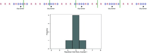
Let us imagine that this polity must be apportioned into six districts of equal size, the boundaries of which are portrayed with vertical bars. Each district contains eight voters, and is hence larger than the scale of the Democratic and Republican clusters. The two parties are evenly matched in four of the resulting districts, which inevitably contain urban, suburban, and rural areas, while the Democrats can expect a majority in one district that ends up slightly more urban, and the Republicans can anticipate a majority in one district that ends up slightly more rural. Thus, the distribution of expected partisanship across districts is symmetric with a large peak in the middle.

Figure 1 indicates that the concentration of voters in cities does not necessarily present a problem for the Democrats. In this example, cities are smaller than the size of districts, but not so small that the Democrats are consistently overwhelmed. Cities are also similar in size and spaced with a uniform distance between them.

Unfortunately for the Democrats, while this hypothetical polity is a useful benchmark for thinking about partisan symmetry, it is not a realistic model for the vast majority of US states. Next, let us examine a political geography that more closely resembles US states with large cities, where instead of being clustered in a series of small agglomerations that do not reach the size of districts, there is at least one cluster that reaches or surpasses that size, along with other smaller agglomerations that do not. For instance, the urban core of New York City is larger than the size of a congressional district, while those of Rochester and Buffalo fall well short. Likewise, urban Memphis approaches the size of a congressional district, while Knoxville and Chattanooga do not. At the scale of state legislative districts, Reading, Pennsylvania is larger than the size of a state lower-chamber district, but the surrounding Democratic railroad towns like Birdsboro are not.

Such a polity is portrayed in Figure 2, which has one large city that votes overwhelmingly for the Democrats, surrounded by heterogeneous suburbs and a rural periphery that vote for the Republicans. It also contains a medium-sized city and a small town, both surrounded by Republican-leaning suburbs and rural periphery.

Fig. 2 Hypothetical polity with cities of different sizes (Example 2).

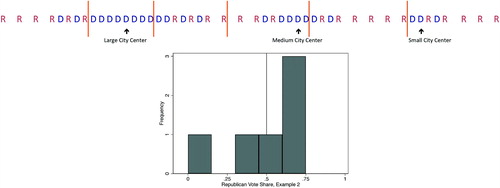
Again, let us examine what happens when this evenly divided polity is partitioned into six districts of equal size. Because Democrats are inefficiently packed into the large city, the cross-district distribution of Republican vote shares has a pronounced left skew, and Democrats win only 42% of the seats in spite of winning half the votes. This is an example of the classic case of electoral bias owing to an inefficient geographic clustering described by Brookes (1960), Johnston (1977), and Gudgin and Taylor (1979).

Next, to get a broader sense of the transformation of votes to seats in this polity, let us consider scenarios in which one of the parties suffers from a scandal or benefits from a strong economy and the election is no longer tied. To do so, we simulate 10,000 elections in which one voter is randomly selected to switch from D to R, then do the same for two voters, three voters, and so on until the R party wins all of the votes. We conduct the same exercise in the opposite direction. For each scenario, we calculate the average seat share across all simulations that would be produced by the districting scheme displayed in Figures 1 and 2. The resulting vote-seat curves are displayed in Figure 3.

Fig. 3 Vote-seat curves for two hypothetical polities.

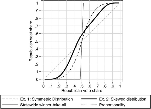
The dashed line in Figure 3 shows simulated seat shares from Example 1. As the figure shows, simulations generate a standard majoritarian vote-seat curve for the polity, which also closely approximates the cube law. For comparison, the dotted line represents proportionality.

The bold line in Figure 3 shows the simulated vote-seat curve for our polity in Example 2. Several features of this curve are noteworthy. First, the curve is flatter and closer to proportionality than the dashed curve from Example 1. Because of the greater relative clustering of the Democrats, the Democratic Party is able to win more seats when it performs badly (on the right side of the graph) than would have been the case with a more even distribution of support across cities. This is because it is able to win seats in its urban core support area even when it performs very badly overall.

Because the support for the Democrats is so concentrated in cities, the Republicans are able to string together suburban and rural voters in districts that they win with slim majorities, and relative to the more even distribution of cities portrayed by the dashed line, they are able to win a seat bonus when they are in the minority, and in the case of a tied election. Of course, the latter case carries considerable normative importance in democratic theory.

The bold curve (Example 2) displays an asymmetry that is not present in the dashed curve (Example 1). In general, the Republican party can expect a larger seat “bonus” than the Democrats—while for some vote shares Democrats get more seats than Republicans in Example 2 than Example 1, on the whole these differences favor Republicans. Most notably, the Republicans can expect a majority of seats with only 45% of the votes. Likewise, they can achieve proportional representation with 40% of the votes, while the Democrats can only expect 30% of the seats with a similar vote share.

3 Measuring Spatial Efficiency

Example 1 captures a scenario in which, even though the Democrats reside in cities, the spatial efficiency of both parties is identical. Example 2 captures a situation in which urban concentration causes the Democrats’ support to be relatively inefficient. The next task is to devise a measure of the parties’ relative support efficiency in a way that facilitates comparisons within states at different spatial scales, and across states with very different levels of support for Democrats and Republicans. Our ultimate goal is to explore how these differences in spatial efficiency translate into representation.

Returning to the two simple examples above, we need not have actually drawn districts to have understood the superiority of the second geographic pattern for the R party. We could also examine each individual voter, and count the number of co-partisans among his or her eight nearest neighbors. In the first example with small, evenly spaced cities, every voter lives in a competitive neighborhood with somewhere between 3 and 5 co-partisans. There are no “landslide” neighborhoods that could give rise to a landslide district. However, in the example with a large city, 75% of the Republicans live in competitive neighborhoods, but only 38% of Democrats do. The large majority of Democrats live in “landslide” neighborhoods with Democratic super-majorities.

We can take this same simple neighborhood-based approach to the US states. We calculate the partisanship of the k nearest neighbors of each voter in each state, where k corresponds to the size of a district in either the state’s lower chamber, upper chamber, or its congressional delegation. Estimation of the partisan composition of each voter’s neighborhood is accomplished through a three-step process. First, precinct-level election returns from the 2008 Presidential election are used to estimate the spatial distribution of voters in each state.³ This is done by creating a number of representative voter points within each precinct, where points are positioned uniformly at random within each precinct’s catchment area, and the number of points in each precinct’s catchment area is proportional to the number of votes cast for each party.⁴ While this introduces two forms of sampling variation—downsampling the number of voters, and the random placement of these voters within each precinct—as shown in the SupplementaryMaterialsSection, the actual variance introduced from these sources is quite small.

The partisan composition of the neighborhood around each of these representative-voter points is then calculated. In the nearest neighbor analysis, for each representative-voter point v of a given party $p\in \{D,R\}$, the partisanship of the neighborhood around v_p is equal to the share of the $N_{\text{state},\mathrm{}\text{chamber}}$ nearest points who are also from party p. The number of nearest neighbors considered—$N_{\text{state},\mathrm{}\text{chamber}}$—is set to ensure the included points represent the number of voters in the average district in the specific chamber of a specific state.⁵ This estimate is analogous to asking “if a circular electoral district of average district population were centered on this voter, what share of people in that district would be co-partisans?” This analysis generates an estimate for each representative-voter point of the share of neighbors who are co-partisans. These point-level estimates can then be aggregated in a variety of ways. Here, we focus on the share of Democratic and Republican voters who reside in competitive vis-a-vis noncompetitive neighborhoods.

To see how such statistics can be illuminating, let us examine a case study of Pennsylvania—one of the most competitive states in presidential and statewide elections in recent years. Figure 4 displays the partisanship of nearest neighbors of Pennsylvania voters at each relevant scale. Voters whose nearest neighbors are extremely Democratic or Republican (over 65%) are displayed in dark blue and red. Highly competitive neighborhoods (in the band between 45 and 55) are displayed in gray.

Fig. 4 The partisanship of nearest neighbors in PA.

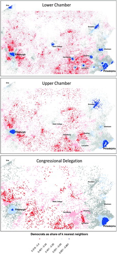
Figure 4 shows that that many urban Pennsylvanians live in landslide Democratic neighborhoods, and many rural dwellers live in landslide Republican neighborhoods. But note the extent to which partisan neighborhoods change from one spatial scale to another. Pennsylvania’s lower-chamber districts are among the smallest in the United States, such that cities like Reading, Allentown, Lancaster, and even York are large relative to the size of districts. As a result, Democrats live in overwhelmingly Democratic neighborhoods in both small and large cities at the scale of the lower chamber. However, at the scale of upper-chamber districts and especially congressional districts, many of these same voters are in neighborhoods that are either competitive or lean Republican. Overall, the share of voters living in competitive neighborhoods increases with spatial scale.

At each spatial scale, the number of red dots is substantially smaller than the number of blue dots. That is, more people live in landslide urban Democratic neighborhoods than in landslide rural Republican neighborhoods. And, as in the stylized example above, Republicans are more likely to reside in competitive neighborhoods. Specifically, at the scale of lower chamber districts, 60% of Republicans live in neighborhoods that are between 40% and 60% co-partisan, but only 52% of Democrats live in such mixed neighborhoods. At the scale of congressional districts, 74% of Republicans live in mixed neighborhoods, but only 59% of Democrats.

The first panel of Figure 5 provides a way to visualize the relative spatial efficiency of the Pennsylvania Republicans at the scale of the state senate. The blue kernel density is the distribution of the Democratic vote share in the neighborhoods of Democrats; the red density is the distribution of Republican vote shares in the neighborhoods of Republicans. We can see that the Republicans have an excellent geographic support distribution. A large share of their voters—69%—are in the competitive zone between 40% and 60% Republican, and they have an especially large density of voters living in neighborhoods that are between 50% and 60% Republican. Democrats, in contrast, have a larger share of their voters living in neighborhoods that are extremely Democratic, and a smaller share living in competitive neighborhoods (only 60%).

Fig. 5 The distributions of partisanship of nearest neighbors of Democrats and Republicans.

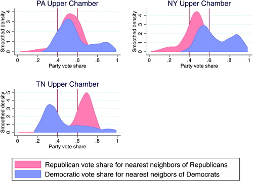
Pennsylvania is an example of a highly competitive state. It is useful to also examine the geographic distribution of partisanship in states that are less competitive. New York is around 60% Democratic, and Tennessee is around 60% Republican. And in both states, Democrats are highly clustered in cities that are larger than the scale of state legislative districts. In the second panel of Figure 5, we see that the Republicans have an enviable distribution of support in New York as well. John McCain’s (adjusted) statewide vote was only 40%, but 70% of those voters were in competitive neighborhoods between the vertical black lines. These neighborhoods are in competitive suburbs and in upstate areas where Democratic industrial towns are small relative to the scale of state senate districts. It is not surprising to find that a large share of Democrats live in neighborhoods where Democrats receive more than the statewide vote share of 60%. What is striking about the distribution in New York, however, is that so few Democrats live in neighborhoods where their co-partisans are in the 60%–70% range. This is because many Democrats live in urban neighborhoods where their co-partisans make up over 70% of the electorate, and a larger share and a large share of Democrats also live in competitive neighborhoods where they are in danger of losing.

The contrast with Tennessee is striking. The Republicans win the same adjusted statewide vote share as the New York Democrats—60%—but none of their voters live in neighborhoods with more than 80% co-partisans. Largely as a consequence of these spatial distributions, from 2008 to 2016, New York Democrats held only half of the seats in the upper chamber of the legislature on average, while Tennessee Republicans held over 70%. Part of the reason why, as these figures show, is that there are almost no Tennessee Republicans living in neighborhoods with more than 80% co-partisans. In other words, rural Tennessee Republican strongholds are more heterogeneous than are New York City Democratic strongholds. Yet very few Tennessee Republicans live in competitive neighborhoods that are in danger of producing Democratic victories. While around 44% of New York Democrats live in competitive neighborhoods, only around 16% of Tennessee Republicans live in such neighborhoods. And for their part, the vast majority of Tennessee Democrats—around 80%—live either in exurban and rural areas where they constitute less than 40% of their neighborhood, or in urban core areas where they constitute well over 60% of their neighborhood.

4 Spatial Efficiency by State

Let us move beyond these case studies and see whether this logic holds up across states. For each state and each legislative scale, we have calculated the share of Democratic voters living in competitive neighborhoods, and the share of Republican voters living in competitive neighborhoods. As in the kernel density graphs above, we characterize competitive neighborhoods as those with an adjusted Obama vote share between 40% and 60%. Results are similar with alternate specifications of the efficiency window.⁶

In Figure 6, we plot efficiency scores for each state and legislative chamber against the statewide vote share for each party at each legislative scale in each state.⁷ In Figure 7, we pool across chambers and fit the data with a local polynomial smoother with 95% confidence intervals. In Figure 7, each state enters the dataset six times, once for each party at each of three legislative scales. In both figures, we drop the congressional observation for states with fewer than four congressional seats, and exclude Nebraska’s state legislature as Nebraska state legislative elections are nonpartisan.

Fig. 6 State values. Notes: Plot present efficiency scores for each party in each state against each party’s overall state-wide vote share, calculated using the two-party vote share in the 2008 Presidential election with a uniform swing adjustment. Plots are separated by Legislative chamber. Figures also include local polynomial regression fits with 95% confidence intervals to reflect uncertainty about how results from this election may generalize to future elections.

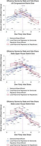
Fig. 7 Share of k nearest neighbors in competitive neighborhoods by party plotted against each party’s overall state-wide vote share, calculated using the two-party vote share in the 2008 Presidential election with a uniform swing adjustment.

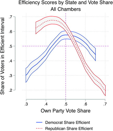
If voters were roughly uniformly distributed, we would expect these scatters to have an inverted U shape. In such a world, when a party receives 50% of the vote, we would expect it to have all voters in competitive, 40%–60% neighborhoods. As a party’s vote share rises, however, the share of their voters in 40%–60% neighborhoods will tend to decline. This inverted U shape is indeed visible in the actual data plotted in Figure 6, but with an interesting asymmetry. As in the New York example above, on the left side of the graph, in states that the Republicans lose, they have very large shares of voters in competitive neighborhoods. When Republicans gain a statewide vote share of only 40%, over 65% of their voters are typically in competitive neighborhoods. In states where Democrats lose by the same margin, less than 40% of their voters are typically in competitive neighborhoods. Moving to the right on the graphs, a gap remains even when we cross the 50% marker. This is especially clear in Figure 7. In other words, Pennsylvania is fairly typical of politically competitive US states in that larger shares of Republicans live in competitive neighborhoods than do Democrats.

Finally, as shown in these polynomial fits, there is a substantial difference between the red and blue lines on the right side of the graph as well. Ideally, a party with more than 60% of the vote, like the Democrats in New York, would like to have its voters spread evenly across neighborhoods, putting it in a position to win all of the seats by a comfortable margin. But if some of its voters are highly concentrated in space, that leaves the rest of its voters in more competitive neighborhoods, providing opportunities for the minority opponent to pick up seats. The Republicans are fortunate: there is a steep decline in the share of their voters living in competitive neighborhoods as their statewide winning margin increases. When Republicans receive 60% of the statewide vote, only around 35% of their voters typically live in competitive neighborhoods. When the Democrats win by the same margin, as described above in the case of the New York State Senate, over half of their voters are typically in competitive neighborhoods, and hence exposed to the possibility of finding themselves in losing districts.

This analysis suggests that the nature of the relative spatial inefficiency faced by Democrats changes with their vote share. In “red” states where they are perennial losers, as well as in highly competitive states, too many of their voters tend to live in “landslide” neighborhoods, and not enough of them live in competitive neighborhoods. However, in many of the “blue” states where they have a commanding majority of votes, too many of their voters tend to live in competitive neighborhoods that they may potentially lose.

5 Spatial Efficiency and Representation

Does the relative spatial efficiency of Republicans have a payoff in seats? To test the role of the spatial efficiency of voters in determining the conversion of total votes to actual legislative seats, we regress the average long-term Republican seat share in the state on the long-term Republican state vote share and voter spatial efficiency. More specifically, we estimate the following OLS model for chamber c in state s:(1) $$\begin{array}{c}R\mathit{epublicanSeatShar}{e}_{c,s}={\alpha }_{c,s}+{\beta }_{0}R\mathit{epublicanVoteShar}{e}_s\\ \mathrm{\hspace{1em}}\mathrm{\hspace{1em}}+{\beta }_1(\mathit{RepublicanEfficienc}{y}_{c,s}*\mathit{RepublicanVoteShar}{e}_s)\\ \mathrm{\hspace{1em}}\mathrm{\hspace{1em}}+{\beta }_2(\mathit{DemocraticEfficienc}{y}_{c,s}*\mathit{RepublicanVoteShar}{e}_s)\\ \mathrm{\hspace{1em}}\mathrm{\hspace{1em}}+{\psi }_{1}R\mathit{epublicanEfficienc}{y}_{c,s}+{\psi }_{2}D\mathit{emocraticEfficienc}{y}_{c,s}\\ \mathrm{\hspace{1em}}\mathrm{\hspace{1em}}+\gamma {\mathit{Z}}_{\mathit{s}}+{ϵ}_{c,s}\end{array}$$(1) where $\mathit{RepublicanSeatShar}{e}_{c,s}$ is the share of seats in chamber c of state s controlled by Republicans from 2008 to 2016,⁸ $\mathit{RepublicanVoteShar}{e}_s$ is the average Republican state-wide Presidential vote share in state s from 2008 to 2016, $\mathit{RepublicanEfficienc}{y}_{c,s}$ is the share of Republican voters whose local neighborhood is between 40% and 60% co-partisan, and $\mathit{DemocraticEfficienc}{y}_{c,s}$ is the share of Democratic voters whose local neighborhood is between 40% and 60% co-partisan.⁹ Z is a set of state dummies.

Our preferred specification for estimating this model is ordinary least squares regression because of its interpretability.¹⁰ Moreover, as shown in the SupplementaryMaterialsSection, the errors from these models are both close to normal and homoscedastic. This is likely due to the fact that Republican seat shares is operationalized by averaging seat shares across several elections, the number of seats in most legislatures is quite large, and parties’ seat shares are rarely near 0 or 1. However, for robustness we also estimate this model using a Binomial regression, which generates similar results as detailed in the SupplementaryMaterialsSection.

We estimate this model on our pooled sample—nearly all states and chambers,¹¹ with and without state fixed effects, and with standard errors clustered at the state level—as well as separately for each chamber.

To ensure reliable estimates of the interaction terms β₁ and β₂, we restrict our analysis to values of Republican vote share for which there is substantial common support for voter efficiency (Hainmueller, Mummolo, and Xu 2018). Given the distribution of voter efficiencies (shown in the SupplementaryMaterialsSection), this amounts to limiting our attention to states with long-run Republican vote shares between 34% and 63%.¹² However, as shown in the SupplementaryMaterialsSection the results that follow are robust to not including this restriction.

We term voters for a party in neighborhoods that support it at a level between 40% and 60% “efficient” because they are not sufficiently clustered to end up in landslide districts, but well enough clustered to potentially elect a winning candidate. Moreover, in addition to having this intuitive rationale, as shown in the SupplementaryMaterialsSection this choice seems to best predict seat shares.¹³ Of course, this is a relatively coarse operationalization of “efficient,” as it does not take into account the distribution of voters outside of the 40%–60% window. As a result, this measure would take on the same value for a party with most voters in 61% neighborhoods as a party with most voters in 90% neighborhoods.¹⁴ Despite this, we use it here due to its ease of interpretation, and show that despite its simplicity, it nevertheless has significant predictive power.

If having voters concentrated in efficient neighborhoods improves a party’s ability to convert their support into seats, then we should see that increasing the share of Republican voters in efficient neighborhoods should increase Republican seat shares (at a given Republican vote share), and increasing the share of Democratic voters in efficient neighborhoods should decrease Republican seat shares (at a given Republican vote share).

The inclusion of an interaction of voter efficiency with overall vote share reflects the fact that voter efficiency is an influence-multiplier, not a direct input into representation. To illustrate, consider a legislature with 10 seats in a state with 100 voters (10 voters per seat). If the Republican vote share is 40%, then a perfectly efficient distribution of Republicans results in Republicans winning six seats.¹⁵ A perfectly inefficient distribution, by contrast, would leave them with only two seats.¹⁶ Consequently, with a 40% vote share, their potential gain from spatial efficiency is four additional seats.

However, if we increase the Republican vote share from 40% to 50%, then a perfectly efficient distribution of Republicans would result in Republicans winning eight seats,¹⁷ while a perfectly inefficient distribution would result in winning only three seats.¹⁸ Thus, the “efficiency bonus” at a 50% vote share would be would be five seats, an increase of 25% over their “efficiency bonus” of four seats at a 40% vote share, an increase proportionate to the increase in overall vote share in this example.

While these examples illustrate the intuition that spatial efficiency will generally increase the representational return for each of a party’s voters, it is important not to press this logic too far. Our measure of spatial efficiency is abstract and divorced from strategic considerations. The fact that a voter is in a neighborhood that is 50% Democratic does not mean that voter will end up in a district that is 50% Democratic for two reasons. First, while our measure can be interpreted as estimating the partisan composition of a voter’s district if that district were circular and centered on the voter,¹⁹ most districts are not circular, and most voters are not at the center of their district. Consequently, it is important not to think of a voter’s spatial neighborhood composition and potential district composition as interchangeable. And second, our analysis abstracts away from strategic considerations entirely. That is, we do not consider the spatial distribution of partisanship in light of possible efforts at incumbency protection, racial representation, or the extent to which clusters of Democrats and Republicans are ripe for strategic packing and cracking.

This simplicity is both a strength and a limitation of our measure. While other measures—such as districting simulations—can accommodate different tuning parameters or technical assumptions (like the specific approach to district construction or definition of compactness used in simulation analyses), this flexibility comes at the cost of model complexity and researcher discretion. As a result, simulation-based measures of gerrymandering require extensive defenses of their underlying technical assumptions, often leading to courtroom battles between opposing expert witnesses that are very difficult for nontechnical audiences to adjudicate.

Our approach, by contrast, gives rise to a simple, transparent baseline political geography model with no tuning parameters, making it more accessible and generalizable. Yet despite its simplicity, our measure of spatial efficiency is nevertheless able to explain a substantial portion of variation in representational inequalities, making clear the central role of spatial clustering in shaping representational inequalities in US legislatures.

Results of this estimation are presented in Table 1. For ease of interpretation, the table include both raw coefficient estimates and a calculated quantity of interest: the estimated marginal partial correlation of voter efficiency and Republican seat share at a 50%/50% overall vote share (${\beta }_1*0.5+{\psi }_1$ for Republicans and ${\beta }_2*0.5+{\psi }_2$ for Democrats).

Table 1 Spatial efficiency and Republican seat shares.

	(1)	(2)	(3)	(4)	(5)
	Pooled	Pooled	State lower	State upper	US House
R average pres vote share 2008–2016	1.53	0	0.28	1.93	3.71
	[0.79, 2.27]	[0, 0]	[–0.87, 1.44]	[0.29, 3.58]	[1.91, 5.51]
R vote share * R share efficient	6.08	4.05	8.10	6.36	0.56
	[2.55, 9.61]	[–12.7, 20.8]	[4.85, 11.3]	[1.95, 10.8]	[–4.87, 5.99]
R vote share * D share efficient	–3.31	–0.45	–4.63	–4.90	0.62
	[–7.55, 0.92]	[–16.1, 15.1]	[–8.16, –1.10]	[–9.46, –0.34]	[–3.73, 4.98]
R share efficient, 50% ± 10	–2.05	–0.87	–3.42	–2.08	0.89
	[–3.89, –0.22]	[–9.24, 7.51]	[–4.91, –1.93]	[–4.21, 0.050]	[–1.83, 3.61]
D share efficient, 50% ± 10	0.90	–0.69	1.81	1.52	–1.06
	[–1.27, 3.07]	[–8.59, 7.21]	[0.14, 3.49]	[–0.64, 3.68]	[–3.18, 1.07]
$\partial \mathrm{R}\mathrm{}\text{seat}\mathrm{}\text{share}/\partial \mathrm{R}\mathrm{}\text{efficiency}$	0.988	1.162	0.624	1.099	1.171
at 50% Vote share	[0.439, 1.537]	[0.055, 2.269]	[–0.030, 1.278]	[0.362, 1.836]	[0.552, 1.790]
$\partial \mathrm{R}\mathrm{}\text{seat}\mathrm{}\text{share}/\partial \mathrm{D}\mathrm{}\text{efficiency}$	–0.756	–0.917	–0.501	–0.930	–0.746
at 50% Vote share	[–1.234, –0.278]	[–2.038, 0.204]	[–1.131, 0.129]	[–1.639, –0.221]	[–1.327, –0.165]
Joint sig. p-values for efficiency vars	0.000	0.093	0.000	0.028	0.009
R-squared	0.673	0.889	0.737	0.605	0.820
SE cluster	State	State
State FE		✓
No. obs.	114	114	41	41	32

NOTE: 90% confidence intervals presented in square brackets. There is no estimate of the coefficient on state-level Republican average Presidential vote share in Column 2 because it is non-time-varying, making it colinear with state fixed effects.

Across specifications, the results show precisely the relationship between spatial efficiency and seats in the legislature predicted by theory. In all five specifications presented, the partial correlation between Republican seat share and the share of Republican voters in efficient neighborhoods in a 50/50 state is positive, and in all five specifications the correlation for Democratic voters is negative. Moreover, in all but one specification, inclusion of measures of spatial efficiency are jointly significant. Most impressively, while the coefficients are not individually significant when state-fixed effects are included, they remain jointly significant, and the point estimates with state fixed effects are stable and in the theoretically predicted direction. This suggests that within states, moving to a spatial scale of representation with greater Republican efficiency is associated with a larger Republican seat share. As shown in the SupplementaryMaterialsSection, results look similar when we use either a wider or a narrower bandwidth to define an “efficient” neighborhood, and the SupplementaryMaterialsSection shows results without the common support restriction. As shown in the regression diagnostics found in the SupplementaryMaterialsSection, these models appear to fit the data well. We also estimate this model using a binomial regression, results of which are similar and can be found in the SupplementaryMaterialsSection.

6 What Is the Role of Gerrymandering?

The preceding analysis makes clear that the spatial distribution of voters plays a role in shaping the transformation of votes into seats. However, the preceding analysis does not imply that all inequalities in the transformation of votes into seats are due to voter geography.

In this section, we use the preceding analysis as a baseline, allowing us to examine the possibility that deliberate political gerrymandering may generate inequalities in representation above and beyond those caused by voter geography. In particular, we examine whether control of the districting process appears to give parties additional advantages in legislative representation even after controlling for the spatial efficiency of voters.

To test for this possibility, we estimate the same simple models as above, focusing only on elections since the last round of redistricting in 2010, and we add dummy variables capturing the partisanship of the entities responsible for drawing district boundaries.²⁰ One indicator variable takes on the value 1 if Democrats had unified control over the redistricting process for the chamber in question after the 2010 census, and zero otherwise. Another indicator variable takes on the value 1 if Republicans had unified control, and zero otherwise. Both of these variables take on the value zero in instances of divided control, independent commissions, or court-drawn plans.²¹

We also include an indicator variable that takes on the value 1 if the state was, at the time of redistricting, required by Section 5 of the Voting Rights Act (VRA) to seek approval from the Department of Justice for any modifications to its electoral laws. Section 5 of the VRA gave the Department of Justice the responsibility to block redistricting proposals that had potential to dilute the ability of minority voters to elect candidates of their choice, and thus constrained the choices of state legislatures.²²

The results of these models are displayed in Table 2. Even after controlling for the overall partisanship of the state and the spatial efficiency of partisanship, the results show that partisan control of districting is associated with improvements in representation for the controlling party. Republican control over the redistricting process is associated with an 10.1 percentage point increase in the Republican seat share among upper chambers, a 5.7 percentage point increase among lower chambers, and an 5.9 percentage point increase among congressional delegations.²³ The coefficients for Democratic control are negative and of similar magnitudes—–8.5, –19.3, –6.4 percentage point for state lower, state upper, and congressional districts, respectively. The coefficients for the VRA variable suggest that controlling for partisan control of the redistricting process and the spatial efficiency of partisanship, states subjected to Section Five oversight had marginally higher Democratic seat shares, though not significantly so.

Table 2 Partisan control and 2012–2016 republican seat shares.

	(1)	(2)	(3)	(4)
	Pooled	State lower	State upper	US House
R average pres vote share 2012–2016	1.46	0.27	1.35	3.63
	[0.59, 2.33]	[–0.58, 1.13]	[0.35, 2.35]	[1.71, 5.56]
R vote share * R share efficient	3.84	5.63	1.37	–0.29
	[1.23, 6.45]	[2.76, 8.49]	[–1.75, 4.48]	[–7.65, 7.07]
R vote share * D share efficient	–1.40	–1.93	–0.13	0.87
	[–5.07, 2.28]	[–5.12, 1.26]	[–3.36, 3.10]	[–4.83, 6.57]
R share efficient, 50% ± 10	–0.99	–2.13	0.037	1.16
	[–2.27, 0.28]	[–3.45, –0.82]	[–1.45, 1.53]	[–2.25, 4.56]
D share efficient, 50% ± 10	–0.044	0.43	–0.63	–1.10
	[–1.85, 1.76]	[–1.11, 1.97]	[–2.18, 0.92]	[–3.68, 1.48]
D districting control	–0.10	–0.085	–0.19	–0.064
	[–0.19, –0.012]	[–0.14, –0.028]	[–0.26, –0.13]	[–0.20, 0.070]
R districting control	0.068	0.057	0.10	0.059
	[0.030, 0.11]	[0.018, 0.096]	[0.058, 0.14]	[–0.052, 0.17]
Covered by VRA	0.021	0.013	–0.034	0.039
	[–0.027, 0.069]	[–0.045, 0.070]	[–0.097, 0.028]	[–0.10, 0.18]
Joint partisan p-value	0.006	0.003	0.000	0.349
SE cluster	State
No. obs.	114	41	41	32

NOTE: 90% confidence intervals presented in square brackets. Dependent variable is Republican share of seats held by Democrats or Republicans between 2012 and 2016.

From this model, we can now answer a slightly different question: for each legislature, how far are actual Republican seat shares from what we might expect if a nonpartisan commission or divided legislature—constrained by existing voter geography—had drawn the legislature’s districts? To answer this question, we calculate the difference, for each legislature, between its actual seat share and the seat share predicted by this model if we were to set all districting control variables to 0. Of course, this does generate a perfect estimate of the outcomes that might be observed under a nonpartisan districting scheme, as party influence over the districting process may occur when parties have less than complete control over the process, but it provides a reasonable strategy for identifying notable outliers.

Consistent with the results in Table 2, the results in Figure 8 clearly show that in states where Republicans control the districting process (red diamonds), they tend to outperform our basic model, and in states where Democrats control the process (blue circles), Republicans under-perform. These graphs make it very clear that the large Republican advantage in many states—especially those in the middle of the distribution and in congressional districts (e.g., Ohio, Wisconsin, Michigan)—cannot be explained by the superior spatial efficiency of support for Republicans alone.

Fig. 8 Difference between actual Republican seat share and Republican seat share based on the model from Table 2.

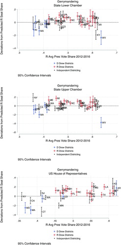
It is especially worthwhile to examine the cases where plaintiffs have filed lawsuits related to partisan gerrymandering. For example, the Wisconsin lower chamber at issue in Gill v. Whitford is a significant outlier in the first plot in Figure 8. This is consistent with the assertion by litigants (supported by simulations) that much of the disproportionate representation of Republicans is explained by efforts to “pack” and “crack” Democrats, and not by an especially inefficient distribution of Democrats.

The third plot in Figure 8 also shows that, as argued in Benisek v. Lamone, the Democratic-drawn redistricting plan in Maryland results in Democrats performing substantially better than would be suggested by the state’s voter geography. The Maryland case illuminates a broader point: while the Democratic party in Maryland has drawn districts that improve on what we might expect given voter geography, the normative implications of this are unclear. Republicans have a highly efficient distribution throughout suburban Maryland, and Democrats are highly concentrated in immediate Washington suburbs and Baltimore, as a result of which the spatial efficiency model predicts a seat share for the Republicans that goes well beyond the cube rule. By drawing a districting plan that produces 7 Democrats out of 8 seats, the Democrats have clearly improved upon what simple voter geography would predict, but in doing so they have brought their representation in line with the expectation of the cube rule, and in line with a seat share that Republicans routinely receive in Southern states where they have similar electoral strength. In other words, these results show descriptively that Democrats may have negated the disadvantage generated by the spatial distribution of their voters; whether this is normatively desirable or not is a distinct question, and one whose answer depends on what one feels is the normative purpose of geographic representation.

7 Conclusion

As indicated in the simple examples above, there is no one-size-fits all indicator of partisan spatial efficiency in a US state. The interaction of district size and city size are such that an arrangement of partisanship that is efficient for the urban party at one scale, for example, that of the state legislative chambers, might be inefficient at another scale like Congress. For instance, small Democratic cities like Fargo are too small and isolated to yield a congressional victory, but the scale of state legislative districts is such that Democrats can expect to win several Fargo seats in the North Dakota state legislature. Moreover, even Democratic cities that are quite small can generate Democratic victories at the scale of congressional districts if they are sufficiently close together, as with New England mill towns, or strings of old industrial towns like Appleton, Neenah, Oshkosh, and Green Bay, Wisconsin. Much also depends on the size and structure of suburbs, and the increasingly poly-centric form of some US cities.

The Democrats have become an overwhelmingly urban political party. Their geographic concentration has increased with each election since the New Deal (Rodden 2019). Something similar is happening in other countries, where parties of the left have come to dominate in poor post-industrial neighborhoods and dense city centers that are connected to the global economy, while parties of the right are more successful in rural and exurban areas.

Thus, in the United States and beyond, due to an inefficient geographic distribution of support, parties that represent cities can be systematically under-represented when single-member districts are drawn, even if those districts are drawn without the intention to produce unequal representation. However, it is also the case that in the United States, districts are often drawn by incumbents bent on providing an advantage for their political party. As a result of these two forces, the under-representation of the Democratic Party in Congress and state legislatures relative to its overall support has become a regular feature of contemporary American politics. Even after the “blue wave” election of 2018, Democrats failed to take control of several state legislatures and Congressional delegations in spite of winning comfortable majorities of votes.

Opponents of partisan gerrymandering have attempted to convince the courts that the practice runs afoul of state and federal constitutions and statutes. The most obvious defense for supporters of partisan redistricting is to claim that since Democrats are inefficiently distributed in cities, large asymmetries in the transformation of votes to seats are to be expected in all states. This article has shown that the Democrats indeed suffer from a relatively inefficient distribution of support in many states, and this has implications for representation. However, the problem is not universal. With the right distribution of city sizes and locations and a fortuitous spatial scale for districting, a party with concentrated urban support can sometimes avoid an inefficient spatial distribution, and suffer no bias in the transformation of votes to seats.

Nor does the spatial inefficiency of Democrats fully explain their under-representation. We have quantified this relative spatial inefficiency at various spatial scales, and demonstrated that when Republican legislators are able to control the process of redistricting, they can increase their party’s representation well beyond that which would be predicted purely from their superior spatial distribution, or create an advantage that would otherwise not exist. Likewise, when the Democrats control the redistricting process, they also appear to create districts to provide them with seat shares above what one might expect given the spatial efficiency of their voters.

Supplementary Materials

Alternative specifications, analyses of sampling variation, and regression diagnostics can all be found in Supplementary Materials online.

Notes

¹ Consider a state with 50 Democratic voters, 50 Republican voters, and 4 districts, each of which must contain the same number of voters. Given the overall distribution of voters, one might expect 2 seats to go to Democrats and 2 to go to Republicans. But one can also create a districting plan where one district has 25 Democrats, two districts have 17 Republicans and 8 Democrats, and one district has 16 Republicans and 9 Democrats. In that configuration, Republicans get 3 seats, and Democrats get 1.

² See, for instance, the “Defendants’ Brief in Support of the Motion to Dismiss” in the original Wisconsin gerrymandering case, Whitford v. Nichol.

³ Because we are attempting to draw inferences about patterns likely to arise in future elections from the results of a single election, we apply a Uniform Swing to normalize for election-specific swings in the Democratic vote share due to candidate effects. In particular, as McCain’s two-party vote share was 46.31%, we apply a 3.69 percentage point uniform swing to all data, so that a Republican voter whose voter neighborhood is 46.31% co-partisan would be said to be in a perfect 50% co-partisan neighborhood. In Congressional races, Democratic victories have been quite rare in districts where McCain’s 2008 vote share was higher than 46.31%, and Republican victories have been quite rare in districts where Obama’s vote share was higher than 53.69%. For a recent overview and defense of the uniform swing assumption, see Jackman (2014).

⁴ In particular, the number of points in each precinct for each party is determined by a draw from a binomial distribution, where n is the number of voters for each party in the precinct. The binomial probability prob varies by state-chamber, but is equal to ${\text{prob}}_k=\frac{\text{number}\mathrm{}\text{of}\mathrm{}\text{districts}}{\text{number}\mathrm{}\text{of}\mathrm{}\text{voters}\mathrm{}\text{in}\mathrm{}\text{state}}*k$, where k = 1000 for state legislative districts and 5000 for US congressional districts. This probability generates k voters per district in expectation. This downsampling makes it computational feasible to calculate the partisan composition each representative voter’s k nearest neighbors. A larger k is used for US congressional districts as they are much larger with respect to individual precincts, resulting in lower binomial draw probabilities for each precinct, thus increasing sampling variance.

⁵ To illustrate, consider a state-chamber with 3 districts and 300,000 voters. The average district is home to 100,000 voters, and so the number of points considered in the nearest neighbor analysis should represent 100,000 voters. Note that because of how prob is constructed, this will amount to examining the share of the 1000 points around each person who are co-partisans for state legislative districts, and 5000 for US congressional districts.

⁶ As discussed in Section 5, in addition to comporting with intuition, the share of co-partisans in the 40%–60% band appears to predict seats shares as well or better than any other band. With that said, results are robust to a number of different center-points and bandwidths, as discussed in the SupplementaryMaterialsSection.

⁷ While we do have the (near) universe of states and 2008 Presidential votes in our data, we feel that the vote data is best thought of as a single draw from a hypothetical super-population of elections, and so we analyze our data using using a frequentist framework.

⁸ Data on state legislative seat shares comes from the National Council on State Legislatures. As compiled seat shares only go back to 2009, data from 2009 is used as an approximation for 2008 seat shares.

⁹ While it may seem intuitive to see Republican Efficiency and Democratic Efficiency as mechanically related, this is not the case. To illustrate, consider a single, square state that is uniformly Democratic on the left and uniformly Republican on the right. Assume the state is large enough with respect to districts that Democrats on the left edge are in 100% Democratic neighborhoods and Republicans on the right edge are in 100% Republican neighborhoods. Now suppose we add more Democratic voters along the left edge of the state–this will drive down the share of Democrats in 40–60% neighborhoods (as the number of Democrats in the middle of the state near Republicans is unchanged, while the number of Democrats in 100% Democratic districts has increased), while leaving the share of Republicans in 40–60% districts unchanged.

¹⁰ Because our primary interest in this analysis is in estimating the marginal effects of voter efficiency, and because we have no theoretical reason to think marginal effects are not relatively constant across the parameter space, a linear model seems most appropriate. Obviously the predicted values from this model may potentially range below 0 or above 1, but as we are not working in a context where it is critically necessary that our predicted values respect the hard boundaries of 0 and 1, we are comfortable accepting this in exchange for interpretability.

¹¹ Due to coarseness of seat shares, US House of Representatives observations do not include states with three or fewer seats in the US House—AK, DE, HI, ID, ME, MT, ND, NH, RI, NE, NM, SD, VT, WY, and WV. Oregon is also excluded from all analyses as all-mail-in elections precluded estimating the spatial distribution of voters using precinct-level returns. Note finally that Nebraska’s state legislative elections are nonpartisan, and for that reason are not included.

¹² The lack of common support for highly Republican and highly Democratic states is unsurprising. In a state that is almost entirely Republicans, for example, most Republicans will necessarily live in neighborhoods that are largely Republican, and thus inefficient. As a result, there are almost no “high efficiency” observations in the tails of the Republican vote share distribution.

¹³ It is worth noting that as described above, for extreme statewide vote shares, having voters in the “efficient” window for 40%–60% is actually potentially inefficient. At a vote share of 80%, for example, an ideal distribution would for all voters to be in 80% neighborhoods, resulting in districts that all have 80% vote shares and thus all have 30% margins against swings in support. In reality, however, given our focus on states between 35% and 65% vote shares, these considerations do not come into play empirically.

¹⁴ A natural extension would be to give all voters scores based how far their neighborhoods deviate from being 50% co-partisan and then sum across all voters.

¹⁵ Six Republicans in each of six districts, four in a seventh, and zero in the remaining districts.

¹⁶ Ten in one district, six in a second, and three in all remaining districts.

¹⁷ Six Republicans in each of eight districts, two and zero in the remaining districts.

¹⁸ Ten, ten, and nine in three districts, three in all others.

¹⁹ Note that if a voter is located near a state boundary, then this simple picture gets a little muddled. The reason is that individuals on the other side of a state border cannot be a part of a voter’s district, and are thus not considered when calculating the Democratic composition of said voter’s nearest neighbors. For a voter located right on the edge of a rectangular state, therefore, we are actually calculating the Democratic vote share of a semicircular hypothetical district with the voter at center-point of the semicircle.

²⁰ We also make a very small adjustment to our sample restriction for common support accordingly—see the SupplementaryMaterialsSection for common support plot for post-2010 data.

²¹ Source: http://redistricting.lls.edu/who.php

²² States covered by Section Five included Alabama, Arizona, Georgia, Louisiana, Mississippi, South Carolina, Texas, and Virginia.

²³ We note, interestingly, that this last estimate is similar to Coriale, Kaplan, and Kolliner’s (2020) estimate (based on a very different type of analysis) that the effect of Republican control over the districting process is a 9.1 percentage point increase in seat share.