A Causal Framework for Observational Studies of Discrimination

Abstract

In studies of discrimination, researchers often seek to estimate a causal effect of race or gender on outcomes. For example, in the criminal justice context, one might ask whether arrested individuals would have been subsequently charged or convicted had they been a different race. It has long been known that such counterfactual questions face measurement challenges related to omitted-variable bias, and conceptual challenges related to the definition of causal estimands for largely immutable characteristics. Another concern, which has been the subject of recent debates, is post-treatment bias: many studies of discrimination condition on apparently intermediate outcomes, like being arrested, that themselves may be the product of discrimination, potentially corrupting statistical estimates. There is, however, reason to be optimistic. By carefully defining the estimand—and by considering the precise timing of events—we show that a primary causal quantity of interest in discrimination studies can be estimated under an ignorability condition that may hold approximately in some observational settings. We illustrate these ideas by analyzing both simulated data and the charging decisions of a prosecutor’s office in a large county in the United States.

Keywords:

• Applications and case studies
• Linear
• Simulation

To assess the role of race or gender in decision making, researchers often examine disparities between groups after adjusting for relevant factors. For example, to measure racial discrimination in lending decisions, one might estimate race-specific approval rates after adjusting for creditworthiness, typically via a regression model. This simple statistical strategy—sometimes called benchmark analysis—has been used to study discrimination in a wide variety of domains, including banking (Munnell et al. 1996), employment (Berg and Lien 2002), education (Baum and Goodstein 2005), healthcare (Balsa, McGuire, and Meredith 2005), housing (Edelman and Luca 2014; Greenberg, Gershenson, and Desmond 2016), and criminal justice (Ayres 2002; Gelman, Fagan, and Kiss 2007; Rehavi and Starr 2014; Fryer Jr 2019; MacDonald and Raphael 2021).

The results of benchmark analyses are often framed in causal terms (e.g., as an effect of race on outcomes), but it is well understood that such an approach suffers from at least three significant statistical challenges when used to estimate causal quantities. First, at a conceptual level, it is unclear how best to rigorously define causal estimands of interest when the treatment is race, gender, or another largely immutable trait. Second, estimates can be plagued by omitted-variable bias if one does not appropriately adjust for all relevant covariates. Third—and the focus of our article—there are worries that estimates are corrupted by post-treatment bias when one adjusts for covariates or restricts to samples of individuals determined downstream from race, gender, or another such treatment variable. This concern, in particular, has raised doubts about the reliability of the literature on police discrimination, where many studies rely on administrative stop records, and hence, implicitly condition on officers stopping an individual, an action that itself is likely discriminatory (Knox, Lowe, and Mummolo 2020; Heckman and Durlauf 2020).

Here we present a causal framework for conceptualizing and estimating a measure of discrimination that is suitable for many applied problems. Our framing specifically addresses concerns about post-treatment bias. To do so, we first define a causal quantity—the second-stage sample average treatment effect, or sate ${}_M$—which closely maps to the legal notion of disparate treatment. For this estimand, by carefully considering the timing of events, we show that treatment assignment conceptually occurs after selection into the sample of interest. We then introduce the notion of subset ignorability, show that this condition formally justifies the use of benchmark analysis to estimate the sate ${}_M$, and discuss settings in which it is likely to hold approximately. We illustrate these ideas by analyzing synthetic data, as well as a detailed dataset of prosecutorial charging decisions for approximately 20,000 felony arrests in a major U.S. county. By developing this statistical foundation, we hope to place discrimination studies on more solid theoretical footing.

1 A Motivating Example

Consider the problem of measuring racial discrimination in prosecutorial charging decisions. After an individual has been arrested, prosecutors in the district attorney’s office read the arresting officer’s incident report and then decide whether or not to press charges. For simplicity, suppose prosecutors only have access to the incident report—and to no other information—when making their decisions. We allow for the possibility that the arrest decision that preceded the charging decision may have suffered from racial discrimination in complex ways that cannot be inferred from the incident reports themselves. Finally, suppose that a researcher has access to these incident reports for arrested individuals, but, importantly, not to any data on individuals that officers considered but ultimately decided against arresting. What, if anything, might one hope to discover about racial discrimination in charging decisions in light of the fact that the people about whom the prosecutor makes charging decisions have been selected—that is, arrested—not randomly, but rather in ways that likely depended on their race?

The first challenge is to rigorously define causal estimands of interest. The inherent difficulty is captured by the statistical refrain “no causation without manipulation” (Holland 1986), since it is often unclear what it means to alter attributes like race and gender (Sekhon 2008). One common maneuver is to instead consider the causal effect of perceived attributes (e.g., perceived race or perceived gender), which ostensibly can be manipulated—for example, by changing the name listed on an employment application (Bertrand and Mullainathan 2004), or by masking an individual’s appearance (Goldin and Rouse 2000; Grogger and Ridgeway 2006; Pierson et al. 2020). In our case, one might imagine a hypothetical experiment in which explicit mentions of race in the incident report are altered (e.g., replacing “white” with “Black”). The causal effect is then, by definition, the difference in charging rates between those cases in which arrested individuals were randomly described (and hence, may be perceived) as “Black” and those in which they were randomly described as “white.” This conceptualization of discrimination conforms to one common causal understanding of discrimination used, for example, in audit studies. This framing also maps closely to the legal notion of disparate treatment, a form of discrimination in which actions are motivated by animus or otherwise discriminatory intent (Goel et al. 2017).

While researchers have carried out such audit studies—including in the case of prosecutorial charging decisions (Robertson, Baughman, and Wright 2019; Chohlas-Wood et al. 2021)¹—it is often infeasible to study important policy questions through randomized experiments. In the absence of a controlled experiment, one can in theory identify this type of causal estimand from purely observational data by comparing charging rates across pairs of cases that are identical in all aspects other than the stated race of the arrested individual.² That strategy, which mimics the key features of the hypothetical randomized experiment described above, is formally justified when treatment assignment (i.e., description of race on the incident report, and subsequent perception by the prosecutor) is ignorable given the observed covariates (i.e., features of the incident report) (Imbens and Rubin 2015). In practice, though, this approach may suffer from omitted-variable bias when the full incident report is not available to researchers, and may suffer from lack of overlap when suitable matches cannot be found for each case—limitations common to many observational studies of causal effects. To address these issues, one can restrict attention to the overlap region and gauge the robustness of estimates to varying forms and degrees of unmeasured confounding (Cornfield et al. 1959; Rosenbaum and Rubin 1983b; Cinelli and Hazlett 2020), an approach we demonstrate below.

Finally, there is the issue of post-treatment bias, especially due to sample selection. Knox, Lowe, and Mummolo (2020) argue that researchers often inadvertently introduce post-treatment bias in observational studies of discrimination by subsetting on apparently intermediate outcomes—such as, in our charging example, being arrested—that themselves may be the product of discrimination. As a result, the authors caution that causal quantities of interest cannot be identified by the data in the absence of implausible assumptions, such as lack of discrimination in the initial arrest decision. In making their argument, Knox, Lowe, and Mummolo focus on the use of force by police officers in civilian encounters, but they suggest their formal critique applies more broadly, casting doubt on a wide range of observational studies of discrimination.

Here we show that such customary subsetting does not pose an insurmountable threat to discrimination research. To understand why, one must precisely define the causal estimand, and carefully consider the timing of events. For instance, in our charging example, there are two relevant treatments, the officer’s perception of race, affecting the officer’s arrest decision, and the prosecutor’s perception of race, affecting the prosecutor’s charging decision. The arrest decision is post-treatment relative to the officer’s perception of race but, importantly, it is pre-treatment relative to the prosecutor’s perception of race. Similarly, the features of the incident report—which we must adjust for in this type of benchmark analysis—are post-treatment relative to the officer’s perception of race but pre-treatment relative to the prosecutor’s perception of race. In such a two-decider situation, as Greiner and Rubin (2011) suggest, it is possible to recover estimates of discrimination by the second decider (e.g., in the charging decision) even if there is discrimination by the first decider (e.g., in the arrest decision).

2 A Measure of Discrimination

We present a simple two-stage model to characterize discriminatory decision making in a variety of real-world situations and define our main causal quantity of interest—the second-stage sample average treatment effect, or sate ${}_M$—within this general framework. In the context of our motivating example, the sate ${}_M$ corresponds to the quantity that would be measured in the hypothetical audit study of prosecutorial decisions described in Section 1. A central aim of this article is to formalize technical assumptions that allow one to statistically identify discrimination—more precisely, disparate treatment—in the second stage (e.g., in prosecutorial charging decisions) when data are only available for individuals who made it past the first stage (e.g., those who were arrested). Importantly, our formalization accommodates scenarios in which first-stage decisions may themselves be discriminatory.

In the first stage, we assume each individual in some population is subject to a binary decision M, such as an offer of employment, admission to college, or law enforcement action. Those who receive a “positive” first-stage decision (e.g., those who are arrested) proceed to a second stage, where another binary decision Y is made. In our running example, the case of each arrested individual is reviewed in the second stage by a prosecutor who may or may not choose to press charges. Those who are not arrested do not have a case that requires review by a prosecutor and, indeed, there may be no administrative record of those individuals.

When considering racial discrimination in decisions involving Black and white individuals, our primary quantity of interest is the second-stage sample average treatment effect, $\mathbb{E}[Y(b)-Y(w)]$, where Y(z) indicates the potential second-stage decision and the expectation is taken over individuals reaching the second stage. Here, we imagine that the perception of race is counterfactually determined after the first-stage decision but before the second-stage decision (e.g., after arrest but before charging, perhaps by altering the description of race on the incident report viewed by a prosecutor). The second-stage sample average treatment effect thus, captures discrimination in the second-stage decision among those who made it past the first stage (e.g., discrimination in charging decisions among those who were arrested). This estimand maps onto a common understanding of disparate treatment in second-stage decisions, including in our charging example.

2.1 A Formal Model of Discrimination

We now formalize the above discussion to explicitly include decisions made at both the first and second stages. For ease of interpretation, we follow Greiner and Rubin (2011) and motivate our statistical model by considering settings where there are two deciders (e.g., an officer and a prosecutor) whose perceptions of race—or gender, or another trait—can in theory be independently altered prior to their decisions. There are, however, examples in which one can plausibly intervene twice even when a single decider makes both decisions. For instance, an officer may decide to stop a motorist based in part on a brief impression of the motorist’s skin tone as they drive past (Grogger and Ridgeway 2006; Pierson et al. 2020). This visual impression of race could subsequently be altered if the motorist presents a driver’s license bearing a name characteristic of another race group, or speaks a dialect of English at odds with the officer’s expectation. It thus may be possible to apply our framework whether one imagines there are two deciders or a single one.

We begin by denoting the race of an individual as perceived by the first decider at the first stage by $D\in \{w,b\}$, where, for simplicity, we consider a population consisting of only white and Black individuals. We focus on racial discrimination for concreteness, but similar considerations apply to discrimination based on other attributes, such as gender. Assuming that there is no interference between units (Imbens and Rubin 2015), we let the binary variables M(w) and M(b) denote the potential first-stage decisions for an individual (e.g., whether they were arrested), and write $M=M(D)$ for the observed first-stage decision. To avoid triviality, we assume throughout that $\mathrm{Pr}(M=1)>0$.

Next, we let $Z\in \{w,b\}$ denote the race of an individual as perceived by the second decider, at the second stage. In our running example, Z denotes race as perceived by the prosecutor reviewing that person’s file, while D denotes race as perceived by the police officer during the encounter. Finally, we define the second-stage potential outcomes as a function of both the first-stage outcome M (e.g., the arrest decision) and the second decider’s perception of race Z. Thus, assuming once again that there is no interference, the observed second-stage outcome for an individual can be denoted $Y=Y(Z,M)$, where we consider four potential second-stage outcomes for each individual: Y(z, m), where $z\in \{w,b\}$ and $m\in \{0,1\}$. In our example, only those who were arrested can be charged, and so $Y(b,0)=Y(w,0)=0$ for all individuals.³

We further allow each individual to have an associated vector of (non-race) covariates X, representing, for example, their behavior during a police encounter, their recorded criminal history, or both. We imagine these covariates are fixed prior to the second-stage treatment (e.g., prior to the prosecutor’s perception of race), since otherwise the key ignorability assumption in Definition 2 below is unlikely to hold. In practice, X is only observed for a subset of the population (e.g., those who were arrested and hence, in the dataset), but we nonetheless define the covariate vector for all individuals in our population of interest. These covariates are not necessary to define our causal estimands of interest, but they play an important role in constructing our statistical estimators.

In this model of discrimination, we have taken care to distinguish between the (realized) first- and second-stage perceptions of race, D and Z, because this helps to clarify the timing of events and the meaning of causal quantities. Importantly, this makes it clear that we can conceive of D and Z as separately manipulable. At the same time, our focus is observational settings, in which disagreement between Z and D may be realized only rarely, if at all, in the data we observe. For instance, barring manipulation of the incident report, it seems unlikely that an arresting officer’s perception of race will frequently differ from a prosecutor’s perception. Our simulation in Section 3 thus imposes the further constraint that perceived race is the same at each stage, though this restriction is not necessary in general.

With this framing, we now formally describe the primary causal estimand we consider. This quantity, which we call the second-stage sample average treatment effect (sate ${}_M$) reflects discrimination in the second stage of the decision-making process outlined above, such as discrimination in the prosecutor’s charging decision.⁴

Definition 1

(sate[INEQ-START). ${}_M$] The second-stage sample average treatment effect, denoted sate${}_M$, is:(1) $${\text{SATE}}_M=\mathbb{E}[Y(b,1)-Y(w,1) | M=1].$$(1)

The estimand in Equation (1)(1) $${\text{SATE}}_M=\mathbb{E}[Y(b,1)-Y(w,1) | M=1].$$(1) compares the potential second-stage decisions under two race perception scenarios. For example, it compares the potential charging decisions when the prosecutor perceives the individual to be either Black or White; importantly, though, the estimand does not explicitly consider the arresting officer’s perception of race. Moreover, this estimand restricts to the subset of individuals who had a “positive” first-stage decision (e.g., those who were in reality arrested).

Because we condition on M = 1 in the definition of the sate ${}_M$, we may equivalently write Equation (1)(1) $${\text{SATE}}_M=\mathbb{E}[Y(b,1)-Y(w,1) | M=1].$$(1) as(2) $${\text{SATE}}_M=\mathbb{E}[Y(b,M)-Y(w,M) | M=1].$$(2)

We can further write(3) $${\text{SATE}}_M=\mathbb{E}[Y(b)-Y(w) | M=1],$$(3) where we define $Y(z)=Y(z,M)$. Among those who reach the second stage (i.e., individuals with M = 1), $Y(z)=Y(z,1)$ denotes the outcome of intervening only on the second decider’s perception of race. Among those who do not reach the second stage (i.e., individuals with M = 0), $Y(z)=Y(z,0)=0$. Equations (1)(1) $${\text{SATE}}_M=\mathbb{E}[Y(b,1)-Y(w,1) | M=1].$$(1) , (2)(2) $${\text{SATE}}_M=\mathbb{E}[Y(b,M)-Y(w,M) | M=1].$$(2) , and (3)(3) $${\text{SATE}}_M=\mathbb{E}[Y(b)-Y(w) | M=1],$$(3) , as well as the informal estimand introduced at the beginning of Section 2, are equivalent ways of capturing the same underlying quantity, varying only in the degree to which they are explicit about the staged nature of the process.

2.2 Estimating the SATE${}_M$

Having defined the sate ${}_M$, our goal is now to estimate it using only second-stage data. That is, we aim to estimate the sate ${}_M$ only using observations for those individuals who received a “positive”—and potentially discriminatory—decision in the first stage. For example, we seek to estimate discrimination in charging decisions based only on data describing those who were arrested. As we show now, an ignorability assumption, together with an overlap condition, is sufficient to guarantee the sate ${}_M$ is nonparametrically identified by data on the second-stage decisions.

Definition 2

(Subset ignorability). We say that $Y(z,1)$, Z, M, and X satisfy subset ignorability if(4) $$Y(z,1)\perp \text{}\perp Z | X,M=1$$(4) for $z\in \{w,b\}$.

In our recurring example, subset ignorability means that among arrested individuals, after conditioning on available covariates, race (as perceived by the prosecutor) is independent of the potential outcomes for the charging decision. As above, we can equivalently write Equation (4)(4) $$Y(z,1)\perp \text{}\perp Z | X,M=1$$(4) as(5) $$Y(z)\perp \text{}\perp Z | X,M=1.$$(5)

This latter expression makes clear that subset ignorability is closely related to the traditional ignorability assumption in causal inference, but where we have explicitly referenced the first-stage outcomes to accommodate a staged model of decision making.

In our prosecutorial setting, subset ignorability would fail if, for example, there were a factor that prosecutors used to make their charging decisions but which was not accounted for in the analysis (e.g., if prosecutors reviewed witness statements that were not in the case files provided to the analyst), and, further, that factor were unbalanced between groups (e.g., if all else equal, witness statements were more commonly available in the cases of white individuals). See Sections 3 and 4 for further discussion of such unobserved confounders and their statistical consequences.

Almost all causal analyses implicitly rely on a version of subset ignorability, since researchers rarely make inferences about the full population of interest. For example, analyses are typically limited to the individuals who agreed to participate in the study. Even randomized experiments, while ideal for internal validity, frequently lack external validity because the study participants do not resemble a larger population of interest. Whenever ascribing causal interpretations to nonexperimental data, it is important to carefully consider the plausability of ignorability and other assumptions, as we discuss in detail in Sections 3 and 4. We note, though, that the assumptions we rely on are similar to those invoked in nearly every observational study of causal effects.

Ignorability assumptions typically require a corresponding overlap condition to guarantee consistent estimation.⁵

Definition 3

(Overlap). We say that overlap holds when $\mathrm{Pr}(Z=z | X=x,M=1)>0$ for all z and x such that $\mathrm{Pr}(X=x,M=1)>0$.

Overlap states that there are no covariate levels for which the probability of receiving one of the treatments is zero within the population of interest. In our prosecution example, overlap ensures that every case has a “twin,” identical in all aspects other than the stated race of the arrested individual, against which it can be compared. Overlap would fail, therefore, in the prosecutorial setting, if, for instance, there were alleged offenses for which only Black individuals were arrested. We note that, unlike ignorability, overlap can be assessed directly from the data; see Section 4. In cases where overlap fails to hold, one can still elicit valid causal estimates by restricting to the subset of the population where overlap holds. For example, in assessing discrimination in prosecutorial charging decisions, one might only consider those alleged offenses for which both Black and white individuals have a nonzero probability of being arrested. But this restriction comes at the cost of inferential validity for the original population. In such cases, one is estimating the causal effect only for the restricted population; the causal effect for the original population may differ, sometimes substantially.

In the traditional, single-stage setting, ignorability and overlap are sufficient to obtain consistent estimates of the average treatment effect. Likewise, we now show that in our two-stage model of discrimination, subset ignorability and overlap are sufficient to guarantee consistent estimates of the sate ${}_M$. In practice, if one can adjust for (nearly) all relevant factors affecting second-stage decisions, one can (approximately) satisfy subset ignorability, and in particular, one can estimate the sate ${}_M$ only using data available at the second stage. In the Appendix, we compare subset ignorability to several alternatives, and show that those variants tend either to be too weak to guarantee identifiability, or unnecessarily demanding for real-world applications. We emphasize that since the first-stage decision, M, and the covariates, X, can be viewed as pre-treatment relative to the second-stage intervention, concerns about post-treatment bias corrupting estimates of the sate ${}_M$ are more naturally thought of as familiar concerns about omitted-variable bias.⁶

Theorem 1.

Suppose $Y(z,1)$, Z, M, and X satisfy subset ignorability and overlap. Then, the sate${}_M$ equals$$\begin{array}{cc}\hfill & \sum _x\mathbb{E}[Y | Z=b,X=x,M=1]·\mathrm{Pr}(X=x | M=1)\hfill \\ \hfill & \hspace{1em}-\sum _x\mathbb{E}[Y | Z=w,X=x,M=1]·\mathrm{Pr}(X=x | M=1).\hfill \end{array}$$

Proof.

Conditioning on X in Equation (1)(1) $${\text{SATE}}_M=\mathbb{E}[Y(b,1)-Y(w,1) | M=1].$$(1) , we have(6) $$\begin{array}{cc}{\mathrm{ }\text{SATE}}_M\hfill & =\sum _x\mathbb{E}[Y(b,1)|X=x,M=1]\hfill \\ \hfill & ·\mathrm{Pr}(X=x|M=1)\hfill \\ \hfill & -\sum _x\mathbb{E}[Y(w,1)|X=x,M=1]\hfill \\ \hfill & ·\mathrm{Pr}(X=x|M=1).\hfill \end{array}$$(6)

By subset ignorability and overlap, we can condition the summands in Equation (6)(6) $$\begin{array}{cc}{\mathrm{ }\text{SATE}}_M\hfill & =\sum _x\mathbb{E}[Y(b,1)|X=x,M=1]\hfill \\ \hfill & ·\mathrm{Pr}(X=x|M=1)\hfill \\ \hfill & -\sum _x\mathbb{E}[Y(w,1)|X=x,M=1]\hfill \\ \hfill & ·\mathrm{Pr}(X=x|M=1).\hfill \end{array}$$(6) on Z = b and Z = w, respectively, without changing their values, yielding(7) $$\begin{array}{cc}{\text{SATE}}_M\hfill & =\sum _x\mathbb{E}[Y(b,1)|Z=b,X=x,M=1]\hfill \\ \hfill & ·\mathrm{Pr}(X=x|M=1)\hfill \\ \hfill & -\sum _x\mathbb{E}[Y(w,1)|Z=w,X=x,M=1]\hfill \\ \hfill & ·Pr(X=x|M=1)\hfill \end{array}$$(7) (8) $$\begin{array}{cc}\hfill & =\sum _x\mathbb{E}[Y(Z,M)|Z=b,X=x,M=1]\hfill \\ \hfill & ·\mathrm{Pr}(X=x|M=1)\hfill \\ \hfill & -\sum _x\mathbb{E}[Y(Z,M)|Z=w,X=x,M=1]\hfill \\ \hfill & ·\mathrm{Pr}(X=x|M=1).\hfill \end{array}$$(8)

Finally, the statement of the proposition follows by consistency, as $Y=Y(Z,M)$. □

Corollary 1.

Suppose subset ignorability and overlap hold, and that we have n iid observations ${(X_i,Z_i,Y_i)}_{i=1}^n$ with M_i = 1. Let $S_x^{(n)}=\{1\le i\le n:X_i=x\}$ represent the set of observations with $X=x$, and let $S_{zx}^{(n)}=\{1\le i\le n:Z_i=z\wedge X_i=x\}$ represent the set of observations with X = x and Z = z. Then the stratified difference-in-means estimator,(9) $$\begin{array}{c}{\Delta }_n=\sum _x\left[\frac{1}{\left|S_{bx}^{(n)}\right|}\sum _{i\in S_{bx}^{(n)}}{Y}_i\right]\frac{\left|S_x^{(n)}\right|}{n}\\ \hspace{1em}-\sum _x\left[\frac{1}{\left|S_{wx}^{(n)}\right|}\sum _{i\in S_{wx}^{(n)}}{Y}_i\right]\frac{\left|S_x^{(n)}\right|}{n},\end{array}$$(9) yields a consistent estimate of the sate${}_M$.

Proof.

Note that by the strong law of large numbers,$$\begin{array}{c}\underset{n\to \infty }{\lim }\frac{1}{\left|S_{zx}^{(n)}\right|}\sum _{i\in S_{zx}^{(n)}}{Y}_i\stackrel{\mathrm{a}.\mathrm{s}.}{=}\mathbb{E}[Y | Z=z,X=x,M=1],\text{and}\\ \underset{n\to \infty }{\lim }\frac{\left|S_x^{(n)}\right|}{n}\stackrel{\mathrm{a}.\mathrm{s}.}{=}\mathrm{Pr}(X=x | M=1).\end{array}$$

Consequently, $\underset{n\to \infty }{\lim }{\Delta }_n$ equals, a.s.,$$\begin{array}{c}\sum _x\mathbb{E}\left[Y\right|Z=b,X=x,M=1]·\mathrm{Pr}(X=x|M=1)\\ \hspace{1em}-\sum _x\mathbb{E}\left[Y\right|Z=w,X=x,M=1]·\mathrm{Pr}(X=x|M=1),\end{array}$$which is the sate${}_M$, by Theorem 1. □

A straightforward calculation further shows that the following expression yields a consistent estimate of the standard error of Δ_n :(10) $$\widehat{\text{SE}}({\Delta }_n)=\sqrt{\sum _x{\left(\frac{\left|S_x^{(n)}\right|}{n}\right)}^2\left[\frac{c_{bx}(1-c_{bx})}{\left|S_{bx}^{(n)}\right|}+\frac{c_{wx}(1-c_{wx})}{\left|S_{wx}^{(n)}\right|}\right]},$$(10) where$$c_{zx}=\frac{1}{\left|S_{zx}^{(n)}\right|}\sum _{i\in S_{zx}^{(n)}}{Y}_i.$$

Equation (10)(10) $$\widehat{\text{SE}}({\Delta }_n)=\sqrt{\sum _x{\left(\frac{\left|S_x^{(n)}\right|}{n}\right)}^2\left[\frac{c_{bx}(1-c_{bx})}{\left|S_{bx}^{(n)}\right|}+\frac{c_{wx}(1-c_{wx})}{\left|S_{wx}^{(n)}\right|}\right]},$$(10) accordingly allows us to form confidence intervals for Δ_n .

The nonparametric stratified difference-in-means estimator Δ_n is the basis for nearly all applications of benchmark analysis in discrimination studies. In practice, as we discuss further in Section 3, it is common to approximate Δ_n via a parametric regression model—but the two estimators share the same theoretical underpinnings. As such, our analysis above simply grounds traditional benchmark analysis within a specific causal framework, and demonstrates that a particular ignorability assumption, together with overlap, is sufficient to yield valid estimates.

2.3 An Alternative Measure of Discrimination

To better understand the sate ${}_M$, we now contrast it with the total effect (te) (Imai, Keele, and Tingley 2010a), a second estimand considered by discrimination researchers (Knox, Lowe, and Mummolo 2020; Heckman and Durlauf 2020; Zhao et al. 2021). The total effect and the sate ${}_M$ differ in our setting in two ways: (a) the population of individuals about which we make inferences; and (b) the potential outcomes being contrasted. The total effect is not restricted to individuals who had a “positive” first-stage decision (e.g., it is not restricted to those who were arrested). Additionally, we imagine a causal variable that reflects a situation where the perception of race is counterfactually determined before the first-stage decision (instead of after the first-stage decision, as with the sate ${}_M$), and is the same at both stages.

We note that, in general—as discussed in Section 1 and below—there is no fully coherent notion of a “total effect” of race, since one cannot intervene on race, per se. In our running example, the two treatments (i.e., the officer’s perception of race and the prosecutor’s perception of race) represent distinct, situation-specific notions of intervening on race. In this restricted context, then, there is a natural estimand that captures the spirit of a “total effect”: comparing an individual’s potential outcomes had they been perceived as white or Black when both the first- and second-stage decisions were made. We formalize this as follows:

Definition 4

(te). The total effect, denoted te, is given by(11) $$\text{TE}=\mathbb{E}[Y(b,M(b))-Y(w,M(w))].$$(11)

Unlike the sate ${}_M$, which only measures discrimination in the second decision, the total effect measures cumulative discrimination across both decisions. In our recurring example, the total effect captures the effect of race at the time of arrest on the subsequent charging decision. In particular, if a charged Black individual had instead been perceived as white by an officer, they might never have been arrested, and hence, never been at risk of being charged, a possibility encompassed by the definition of the total effect, but not by the sate ${}_M$.

We stress, however, that in studies of discrimination—particularly racial discrimination—there is often no clear intervention point, and the difference between the te and the sate ${}_M$ is largely an artifact of how one defines both the population of interest and the start of the decision-making process. What is the te in one description of events may be the sate ${}_M$ in another, equally valid description of the same events, as we describe next.

In our running example, the implicit population of interest consists of those individuals stopped by the police, and the te reflects a description of events in which the decision-making process starts—and perception of race is counterfactually determined—when the arrest decision is made. We can, however, imagine moving back the clock and starting the process when the stop decision is made, with the population of interest now comprising those individuals spotted by an officer. In this case, the original te is equivalent to the sate ${}_M$ on this newly defined population, where the first-stage decision indicates whether an individual was stopped. Both the original te and the new sate ${}_M$ capture combined discrimination in the arrest and charging decisions, among the subset of individuals who were stopped.⁷

But the moment when an individual is spotted is no more statistically privileged as a starting point than the moment when an officer makes a stop decision. One could similarly measure cumulative discrimination that includes the stop decision itself, either in terms of the te or the sate ${}_M$. For the te, as above, we imagine time starting immediately after a potential police encounter, with the first-stage decision indicating whether an individual was stopped (among a population of individuals spotted by the officer). 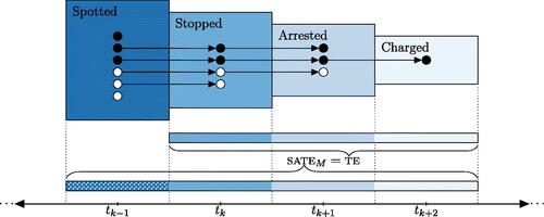For the sate ${}_M$, we back up the clock once again and imagine the first-stage decision indicating whether an individual was spotted by an officer, among an even larger population of people walking through the neighborhood where the officer patrols. Figure 1 provides a graphical depiction of this interchangeability.⁸

Fig. 1. This figure illustrates estimands one could consider, and the populations they concern, as individuals move through one segment of the criminal justice system. For instance, one can measure combined discrimination in arrest and charging decisions either via the te or the sate ${}_M$. In studies of discrimination, there is no clear point at which race is “assigned” and so both the te and the sate ${}_M$ can be used interchangeably to express the same underlying causal effect, the te with respect to the population of stopped individuals, and the sate ${}_M$ with respect to the population of spotted individuals. More generally, the diagram illustrates a multistage process, where one seeks to measure discrimination culminating at stage $t_{k+2}$ (e.g., charging decisions) among those who make it to stage t_k (e.g., those who were stopped by the police). This quantity can be viewed as the te, where one imagines the process starting at time t_k . Alternatively, it can be viewed as the sate ${}_M$, where one views the process as starting earlier (at, say, $t_{k-1}$, indicating that an officer spotted an individual), and then conditioning on those who made it to stage t_k . Note that the quantities themselves are formally defined—and equivalent in the manner just described—even absent any considerations of estimation and randomization, which are not illustrated here.

Although the te may appear to avoid conditioning on intermediate outcomes, it simply masks a complex chain of events that came before the nominal start of the process, a chain that itself was likely influenced by discriminatory decisions. For instance, the officer spotting and stopping motorists in our running example could be patrolling the neighborhood in question because of its racial composition.⁹ The very idea of “intermediate outcomes”—a concept central to concerns about post-treatment bias—is a slippery notion in the context of discrimination studies, where there is no clear point in time where one can imagine that race is “assigned.” Even birth cannot be considered the ultimate starting point since, in theory, one might include, at the least, the race of a child’s parents, determined at an earlier stage, when assessing discrimination.¹⁰ Indeed, such generational counterfactuals may be critical for understanding systemic, institutional discrimination.

Our discussion of discrimination in multi-staged, multi-decider scenarios applies widely, but it is not universal. In particular, measuring discrimination in a single-decider case—and, specifically, in officer use of force—is challenging. In many of these single-decider scenarios, it is hard to imagine intervening on race after the decision-making process begins, making it difficult to isolate discrimination in later stages.

3 Assessing Second-Stage Discrimination in a Stylized Scenario

Subset ignorability, in theory, is sufficient to ensure nonparametrically identified estimates of the sate ${}_M$, even when the first-stage decisions are discriminatory. We illustrate that idea by investigating in detail a hypothetical scenario involving discriminatory arrest decisions in the first stage and discriminatory charging decisions in the second stage. We explore the properties of simple estimators in this setting through a simulation study. We demonstrate that failing to adjust for a factor that directly influences charging decisions can result in biased estimates of discrimination in those decisions, but by accounting for all factors that directly influence charging decisions—and hence, satisfying subset ignorability—one can accurately estimate the sate ${}_M$, even when there is unmeasured confounding in arrest decisions. This example further clarifies the conceptual importance of distinguishing between an officer’s perception of race and a prosecutor’s perception of race when defining and estimating our quantities of interest.

We consider a hypothetical jurisdiction in which police officers observe the behavior and race of individuals who are potentially engaged in specific criminal activity (e.g., a drug transaction) and then decide whether or not to make an arrest. Subsequently, the case files of arrested individuals—consisting of a written copy of the officer’s description of the encounter and the arrested individual’s criminal history—are brought to a prosecutor who decides whether or not to press charges. We assume the prosecutor only observes the documented race and criminal record of the arrestee, and the arresting officer’s written description of the encounter; accordingly, by construction, the charging decision depends only on these three factors. For example, the prosecutor may choose only to charge individuals who have several previous drug convictions and who were reported to be engaging in a drug transaction. Importantly, while the prosecutor has access to an officer’s written report, the prosecutor does not directly observe the individual’s behavior leading up to the arrest.

Our goal is to estimate discrimination in charging decisions, formalized in terms of the sate ${}_M$. Intuitively, if we observe every arrested individual’s criminal history, race, and officer report, then subset ignorability would hold because the prosecutor’s charging decision depends only on these factors. Thus, with these three covariates, we could generate valid estimates of discrimination in prosecutorial decisions, even without knowing all of the factors that led to an arrest, a decision that may itself have been discriminatory. However, if any of these three covariates—criminal history, race, or officer report—are unobserved, we will, in general, be unable to accurately assess discrimination in prosecutorial decisions. In both scenarios, with and without unmeasured confounding, our analysis is based on the subpopulation of arrested individuals, where we note that the subsetting (i.e., arrest) is not influenced by the prosecutor’s perception of race. In this setting, the primary concern is thus omitted-variable bias, not post-treatment bias.

We emphasize that we seek only to estimate discrimination in the second-stage charging decision, not cumulative discrimination stemming from both the arrest and charging decisions. In particular, while officer reports may represent an inaccurate—and discriminatory—account of events, such discrimination is distinct from that in the charging decision itself. Similarly, criminal histories reflect a form of complex, long-term discrimination that we do not aim to measure here. Alternative, and more expansive, notions of discrimination are important to understand, but here we focus on assessing the prosecutor’s narrow contribution to inequities at a specific point in the process, a common statistical objective closely tied to policy decisions and legal theories of disparate treatment (Jung et al. 2018).

3.1 The Data-Generating Process

We now formally describe the data-generating process for our stylized example. Under the structural causal model we consider, we can both compute the true sate ${}_M$ and compute estimates based only on select information available to the prosecutor. In defining the generative process, we closely follow the terminology and conventions of Pearl (2009) and Pearl, Glymour, and Jewell (2016).¹¹

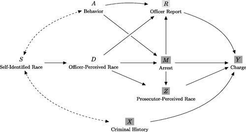
Our model is defined in terms of the causal directed acyclic graph (DAG) depicted in Figure 2. In this model, $S\in \{w,b\}$ indicates one’s self-identified race, and D and Z indicate, respectively, an officer’s and a prosecutor’s perception of race. Further, $M\in \{0,1\}$ indicates the arrest decision, and $Y\in \{0,1\}$ indicates the charging decision. Finally, A corresponds to an individual’s behavior, as observed by an officer, and X and R correspond, respectively, to criminal history and an officer’s description of an encounter, as included in the arrest report. For simplicity, in our example these latter three variables are operationalized as being binary—for example, one can imagine that X indicates whether an individual had at least one previous drug conviction, A indicates whether they were seen actively engaging in a drug transaction, and R indicates whether they were reported by the officer to be actively engaging in a drug transaction. Officers observe D, A, and R for all individuals; prosecutors observe Z, X, and R only for the subset of arrested individuals. Note that we also allow for Z and R to be missing (i.e., to take the value $\text{NA}$) in cases where an individual is not arrested.

Fig. 2. A causal DAG depicting our stylized example of arrest and charging decisions, where D represents the officer’s perception of race, and Z represents the prosecutor’s perception of race. Officer arrest decisions (M) are directly influenced by observed criminal behavior (A) and officer-perceived race (D); the officer reports of the encounters (R) are directly influenced by A and D. Prosecutorial charging decisions are made for all arrested individuals, and are directly influenced by officer reports (R), criminal history (X), and prosecutor-perceived race (Z). Finally, an individual’s self-identified race (S) influences the officer’s perception of race (D), and is confounded with criminal history (X) and behavior (A). We consider two scenarios. The variables highlighted in dark gray (i.e., M, Z, X, and Y) are always observed. In one scenario, the analyst also observes the officer report R, highlighted in light gray, obtaining the full set of information available to the prosecutor; in the other, the analyst does not observe the officer report R (i.e., only M, Z, X, and Y are observed), leading to omitted-variable bias.

Structural causal models are defined by a set of exogenous random variables and deterministic structural equations specifying the values of all other variables in the DAG. In our example, the independent exogenous variables are:$$\begin{array}{c}{U}_L\sim \text{BERN}({\mu }_L),\\ U_A,U_M,U_X,U_R,U_Y\sim \mathrm{ }\text{UNIF}(0,1),\end{array}$$where μ_L is an appropriately defined constant.

We define self-identified race (S), behavior (A), and criminal history (X) in terms of U_L , which captures latent confounding. For constants μ_A , γ, μ_X , and δ, the structural equations for these three variables are given by$$\begin{array}{c}{f}_S(u_L)=\{\begin{array}{cc}w\hfill & u_L=0,\hfill \\ b\hfill & u_L=1,\hfill \end{array}\\ f_A(u_A,u_L)=1(u_A\le {\mu }_A+\gamma ·u_L),\\ f_X(u_X,u_L)=1(u_X\le {\mu }_X+\delta ·u_L).\end{array}$$

This specification allows for the distributions of criminal history and behavior to vary by race due to exogenous factors like disparate police deployment and historical discrimination. For example, stopped Black individuals may be less likely to be engaged in criminal activity than stopped white individuals, corresponding to $\gamma <0$.

In line with our discussion in Section 2.1, we set the prosecutor’s perception of race (Z) equal to the officer’s perception of race (D), and, for simplicity, we set both equal to one’s self-identified race (S). This choice yields the following structural equations:$$\begin{array}{c}{f}_D(s)=s,\\ f_Z(m,d)=\{\begin{array}{cc}d\hfill & m=1,\hfill \\ \text{NA}\hfill & m=0.\hfill \end{array}\end{array}$$

Note that, when someone is not arrested, we represent the prosecutor’s perception of race as an explicit missing value. The arrest report, R, is treated similarly below.

Finally, for constants α₀, α_A , ${\alpha }_{\text{black}}$, λ₀, λ_A , ${\lambda }_{\text{black}}$, β₀, β_X , β_R , and ${\beta }_{\text{black}}$, the structural equations for arrest decisions (M), police reports (R), and charging decisions (Y) are given by$$\begin{array}{c}{f}_M(d,a,u_M)\\ =1(u_M\le {\alpha }_0+{\alpha }_A·a+{\alpha }_{\text{black}}·1(d=b)),\\ f_R(d,a,m,u_R)\\ =\{\begin{array}{cc}1(u_R\le {\lambda }_0+{\lambda }_A·a+{\lambda }_{\text{black}}·1(d=b))& m=1,\\ \text{NA}& m=0,\end{array}\\ f_Y(z,m,r,x,u_Y)\\ =\{\begin{array}{cc}1(u_Y\le {\beta }_0+{\beta }_X·x+{\beta }_R& \\ · r+{\beta }_{\text{black}}·1(z=b))& m=1\wedge z\ne \text{NA}\wedge r\ne \text{NA},\\ \text{NA}& m=1\wedge (z=\text{NA}\vee r=\text{NA}),\\ 0& m=0.\end{array}\end{array}$$

In particular, arrest decisions and police reports depend on an officer’s perception of race, whereas charging decisions depend on a prosecutor’s perception of race. This model incorporates both discrimination in arrest decisions, via ${\alpha }_{\text{black}}$, and discrimination in police reports—for example, by omitting potentially exculpatory details or by falsifying information—via ${\lambda }_{\text{black}}$. Discrimination in charging decisions is encoded by ${\beta }_{\text{black}}$.

The above structural equations, together with the distributions on the exogenous variables, fully define the joint distribution of realized and potential outcomes. In particular,$$\begin{array}{cccc}S\hfill & =f_S(U_L),\hfill & D\hfill & =f_D(S),\hfill \\ Z\hfill & =f_Z(M,D),\hfill & A\hfill & =f_A(U_A,U_L),\hfill \\ X\hfill & =f_X(U_X,U_L),\hfill & M\hfill & =f_M(D,A,U_M),\hfill \\ R\hfill & =f_R(D,A,M,U_R),\hfill & Y\hfill & =f_Y(Z,M,R,X,U_Y).\hfill \end{array}$$

The primary causal quantity we seek to estimate—the sate ${}_M$—is defined in terms of counterfactuals Y(z, m). As discussed in Pearl (2009) and Pearl, Glymour, and Jewell (2016), such counterfactuals require some care to define, as one must appropriately account for the exogenous variables U. In particular, for the causal DAG in Figure 2, the bivariate charge potential outcomes, for counterfactual versions of prosecutor-perceived race, are given by $Y(z,m)=f_Y(z,m,R(m),X,U_Y)$, where $R(m)=f_R(D,A,m,U_R)$ are the counterfactual versions of the officer report. Further, the arrest potential outcomes—where we consider counterfactual versions of officer-perceived race—are given by $M(d)=f_M(d,A,U_M)$. In general, counterfactuals defined in this way obey the consistency rule, meaning that $M=M(D)$ and $Y=Y(Z,M)$.

When ${\alpha }_{\text{black}}\ge 0$, anyone who would be arrested if white would also be arrested if Black (i.e., $M(b)\ge M(w)$). When ${\alpha }_{\text{black}}>0$, we say arrest decisions are discriminatory since, all else being equal, an individual is more likely to be arrested if they were Black than if they were white. Likewise, $Y(b,1)\ge Y(w,1)$ when ${\beta }_{\text{black}}\ge 0$, meaning that an individual who would be charged if arrested and white would also be charged if arrested and Black. We say the charging decision is discriminatory when ${\beta }_{\text{black}}>0$.

3.1.1 Features of Our Data-Generating Process

Table 1 displays a sample of five rows of data generated from our model. From the full set of potential outcomes, we can compute the true sate ${}_M$ by directly applying Definition 1 to the generated data, taking the average difference between $Y(b,1)$ and $Y(w,1)$ among arrested individuals.¹² However, given the simple linear form of our structural equations, a straightforward calculation also shows that the sate ${}_M$ is exactly equal to ${\beta }_{\text{black}}$.

Table 1. A sample of potential and realized outcomes for individuals in our hypothetical example.

S	D	A	X	M(b)	M(w)	M	Z	R	R(0)	R(1)	$Y(b,1)$	$Y(w,1)$	Y
b	b	0	0	0	0	0	$\text{NA}$	$\text{NA}$	$\text{NA}$	0	0	0	0
b	b	0	1	0	0	0	$\text{NA}$	$\text{NA}$	$\text{NA}$	1	1	0	0
b	b	1	1	1	0	1	b	10	$\text{NA}$	0	1	1	1
w	w	0	0	1	1	1	w	1	$\text{NA}$	1	0	0	0
w	w	0	1	0	0	0	$\text{NA}$	$\text{NA}$	$\text{NA}$	0	0	0	0

Note: The data-generating process produces the full set of entries, but the prosecutor only observes the realized outcomes for those who were arrested, indicated by the shaded cells. In the first scenario we consider, the analyst also observes all the information in the shaded cells; in the second scenario, the analyst only observes the information in the dark gray cells (i.e., the analyst does not observe the officer report R), leading to omitted-variable bias.

Table D.1 Breakdown of charges, prior arrests, and prior convictions, and weapons involvement among individuals arrested for a felony offense between 2013 and 2019 in a major U.S. county, as analyzed in Section 4.

		Male	Female	Black	White
Charge	arson	50	218	79	124
	assault	2062	9160	4131	3662
	burglary	664	3334	1762	1535
	burglary (auto)	125	1216	737	338
	driving under the influence	26	90	17	50
	drug-related offense	736	5643	2815	1881
	forcible rape	3	112	49	26
	forgery	60	187	103	84
	hit-and-run	10	42	18	17
	kidnapping	4	24	12	1
	manslaughter (vehicular)	2	8	4	3
	motor vehicle theft	83	323	161	141
	other felony offense	287	2115	877	910
	other sex offense	8	180	85	54
	robbery	458	2186	1536	589
	theft	877	3385	1723	1539
	weapons offense	80	882	513	218
	willful homicide	53	178	65	60
Prior arrests	0	3192	13,491	5881	5682
	1	1005	5486	2972	1977
	2	553	3315	1929	1134
	3	321	2199	1215	786
	4	191	1558	895	540
	5	116	1066	591	364
	6	78	697	381	242
	7	40	469	248	157
	8	29	316	180	103
	9	18	204	111	84
	10+	45	482	283	163
Prior convictions	0	4451	20,775	9937	8290
	1	748	5221	2961	1773
	2	278	2055	1111	730
	3	78	766	429	261
	4	23	312	171	116
	5+	10	154	77	62
Weapons	no weapon involved	4442	24,932	12,810	9434
	weapon involved	1146	4351	1876	1798

Note: Note that only Black and non-Hispanic white individuals are analyzed in our race-based analysis, so within-row sums differ between race and gender.

Our hypothetical example captures three key features of real-world discrimination studies. First, prosecutorial records do not contain all information that influenced officers’ first-stage arrest decisions (i.e., prosecutors only observe R, not A). Second, our set-up allows for situations where the arrest decisions are themselves discriminatory—those where ${\alpha }_{\text{black}}>0$—or the officer’s report is discriminatory, for example, because of omission of exculpatory information or deliberate falsification—those where ${\lambda }_{\text{black}}>0$. Third, the prosecutor’s records include the full set of information on which charging decisions are based (i.e., Z, X, and R).

Among those who were arrested, the charging potential outcomes depend only on one’s criminal history (X) and the arrest report (R). In particular, they do not depend on one’s realized, prosecutor-perceived race (Z). Consequently, $Y(z,1)\perp \text{}\perp Z | X,R,M=1$, meaning that the model satisfies subset ignorability relative to X and R. As a result, access to X and R, along with overlap, guarantees the stratified difference-in-means is a consistent estimator of the sate ${}_M$, even if one does not have access to A.¹³ However, in general, $Y(z,1)\cancel{\perp \text{}\perp }Z | X,M=1$ (and, likewise, $Y(z,1)\cancel{\perp \text{}\perp }Z | R,M=1$), and so if one only has partial information on charging decisions there is no guarantee the sate ${}_M$ can be consistently estimated.¹⁴ Indeed, when there is such unmeasured confounding in the prosecutor’s decisions, one should expect biased estimates of the sate ${}_M$.

3.2 Estimating the SATE${}_M$

Although the data-generating procedure produces the full set of potential outcomes for each individual, the prosecutor only observes a subset of the cells—realized outcomes for arrested individuals, highlighted in gray in Table 1. While this circumscribes the causal effects one can estimate—for example, discrimination by police will no longer be identifiable in the reduced dataset—one can still learn about the sate ${}_M$. We explore the performance of two statistical methods for estimating the sate ${}_M$ based on data observed by the prosecutor: the stratified difference-in-means estimator described in Equation (9)(9) $$\begin{array}{c}{\Delta }_n=\sum _x\left[\frac{1}{\left|S_{bx}^{(n)}\right|}\sum _{i\in S_{bx}^{(n)}}{Y}_i\right]\frac{\left|S_x^{(n)}\right|}{n}\\ \hspace{1em}-\sum _x\left[\frac{1}{\left|S_{wx}^{(n)}\right|}\sum _{i\in S_{wx}^{(n)}}{Y}_i\right]\frac{\left|S_x^{(n)}\right|}{n},\end{array}$$(9) , and a regression-based estimator. We apply each of these methods to two types of data: the full set of information available to prosecutors (i.e., Y, Z, X and R), and an incomplete dataset comprised only of Y, Z, and X (highlighted in dark gray in Table 1), in which case we view R as an unmeasured confounder.

One can compute the stratified difference-in-means estimate in three steps. First, partition arrested individuals into subsets that have the same value of the available control variables (i.e., X and R in the complete data setting, and X alone in the partial data setting). Second, on each resulting subset, compute the average difference in charging rates between Black and white individuals. Third, take a weighted average of these differences, where the weights reflect the proportion of arrested individuals in each subset. In addition, one can apply Equation (10)(10) $$\widehat{\text{SE}}({\Delta }_n)=\sqrt{\sum _x{\left(\frac{\left|S_x^{(n)}\right|}{n}\right)}^2\left[\frac{c_{bx}(1-c_{bx})}{\left|S_{bx}^{(n)}\right|}+\frac{c_{wx}(1-c_{wx})}{\left|S_{wx}^{(n)}\right|}\right]},$$(10) to estimate the standard error of this point estimate to generate confidence intervals.

The stratified difference-in-means estimator is theoretically appealing in that it is guaranteed to yield consistent estimates of the sate ${}_M$ when subset ignorability and overlap hold. But the estimator can have high variance when the dimension of the covariate space is high and the sample size is small. Thus, in practice, it is common to model potential outcomes as a function of observed covariates—also known as response surface modeling (Hill 2011). In particular, on the subset of arrested individuals, one can estimate the sate ${}_M$ via a parametric model that estimates observed charging decisions as a function of the available information.

To demonstrate this latter approach, we use a linear probability model. In the complete data setting, we have:(12) $$\mathbb{E}[Y | Z,X,R]={\beta }_0+{\beta }_{1}Z+{\beta }_{2}X+{\beta }_{3}R,$$(12) where the model is fit on the full set of arrests seen by the prosecutor. Under this model, the sate ${}_M$ is approximated by the fitted coefficient ${\widehat{\beta }}_1$, since that term captures the difference in charging potential outcomes after adjusting for the observed covariates. For our specific stylized example, the linear regression model in Equation (12)(12) $$\mathbb{E}[Y | Z,X,R]={\beta }_0+{\beta }_{1}Z+{\beta }_{2}X+{\beta }_{3}R,$$(12) is in fact perfectly specified—exactly mirroring the prosecutor’s charging decisions—and so we are guaranteed to obtain statistically consistent estimates. In the partial data setting, where an analyst only has access to X, one must fit a reduced model that excludes R:(13) $$\mathbb{E}[Y | Z,X]={\beta }_0+{\beta }_{1}Z+{\beta }_{2}X.$$(13)

In this case, ${\widehat{\beta }}_1$ in general yields a biased estimate of the sate ${}_M$, because of the omitted variable R. The stratified difference-in-means estimator will in general similarly yield a biased estimate of the sate ${}_M$ in this omitted-variable setting.

3.3 Simulation Results

We perform a simulation study to understand the properties of the above estimators, varying our assumptions about discrimination and confounding. We simulate 10,000 datasets of size 100,000 for each of 25 different parameter settings. Each setting is defined as a combination of our two key discrimination parameters, ${\alpha }_{\text{black}}$ and ${\beta }_{\text{black}}$, where each parameter is allowed to take one of five values: 0.20, 0.25, 0.30, 0.35, and 0.40. Across all simulation settings, we assume the population of individuals encountered by police is 30% Black (i.e., ${\mu }_L=0.3$); that 30% of white individuals and 40% of Black individuals have a past drug conviction, indicated by X; and that 30% of white individuals and 20% of Black individuals are seen engaging in a drug transaction, indicated by A.¹⁵ These settings allow for a substantial amount of overlap across race groups with regard to the key covariates.

On each synthetic dataset, we estimate the sate ${}_M$ using both the stratified difference-in-means estimator and the regression-based estimator, and compare the results to the true population-level sate ${}_M$ in two scenarios. To illustrate the impact of omitted variable bias, in the first scenario, we assume the officer’s report R is unavailable—meaning there is unmeasured confounding—and therefore, only stratify based on X in the difference-in-means estimator, and fit the model in Equation (13)(13) $$\mathbb{E}[Y | Z,X]={\beta }_0+{\beta }_{1}Z+{\beta }_{2}X.$$(13) for the regression-based estimator. In the second scenario, we assume that R is available, and stratify on both X and R in the difference-in-means estimator, and fit the model in Equation (12)(12) $$\mathbb{E}[Y | Z,X,R]={\beta }_0+{\beta }_{1}Z+{\beta }_{2}X+{\beta }_{3}R,$$(12) for the regression-based estimator. For each combination of ${\alpha }_{\text{black}}$ and ${\beta }_{\text{black}}$, the estimates on the 10,000 synthetic datasets yield the approximate sampling distributions for the difference-in-means and regression-based estimators. In Figure 3, we summarize each sampling distribution by its mean, 2.5th percentile, and 97.5th percentile. The solid points correspond to the difference-in-means estimator, and the hollow points to the regression-based estimator. The horizontal lines indicate the true population-level sate ${}_M$.

Fig. 3. In our hypothetical example of officer and prosecutor behavior, estimates of discrimination in charging decisions are biased when information directly influencing those decisions—in this case, an officer’s report—is omitted (left). However, one can obtain accurate estimates of discrimination when accounting for all information directly influencing charging decisions (right). Each plot shows the results of 10,000 simulations for each of 25 different combinations of discrimination in officer and prosecutor decisions, given by ${\alpha }_{\text{black}}$ and ${\beta }_{\text{black}}$, respectively. The true value of the sate ${}_M$, indicated by the horizontal colored lines, is computed based on the full set of potential outcomes for each individual, and does not depend on the degree of discrimination in the first stage, as seen by the constant value of the sate ${}_M$ across different values of ${\alpha }_{\text{black}}$. For each parameter choice, we display the mean of the sampling distribution for the stratified difference-in-means estimator (solid circle) and the regression-based estimator (hollow circle), along with the interval spanned by the 2.5th and 97.5th percentiles of the sampling distribution. In the right plot (“unconfounded”), estimates are based on all three factors that directly influence charging decisions: race, criminal history, and officer report; in the left plot (“confounded”), we omit the report. When all variables directly influencing charging decisions are available, both estimators recover the true value of the sate ${}_M$, even when there is an unknown degree of discrimination in arrest decisions.

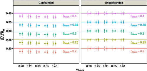
In the left panel (“confounded”) of Figure 3, the points lie below the horizontal lines in all cases, meaning we underestimate discrimination in charging decisions. In this setting, estimates do not account for the officer reports R, and so there is unmeasured confounding in the charging decisions. We set $\gamma <0$ in our simulations, and thus, stopped and arrested Black individuals are less likely to be engaging in criminal activity, a pattern (noisily) reflected in the officer reports. Because we assume these arrest reports are not available for analysis, we cannot fully adjust for their direct influence on prosecutor decisions. As a result, by adjusting for X alone, we miss an important, unmeasured difference between arrested white and Black individuals, leading us to underestimate discrimination in prosecutorial decisions.

In the right panel (“unconfounded”) of Figure 3, the points lie on the horizontal lines in all cases, meaning the estimators are unbiased, and the range between the 2.5th and 97.5th percentiles is relatively narrow, indicating estimates are typically close to the true value. These results hold even when one is unable to assess the degree of discrimination ${\alpha }_{\text{black}}$ in the arrest decisions. As implied by Theorem 1, to accurately estimate the sate ${}_M$, it is sufficient to measure all covariates that directly influence the prosecutor’s decisions. In practice, it is nearly always impossible to do so perfectly; for instance, decision factors such as forensic evidence may not be readily available, or non-obvious factors, such as the time of day, may play a role in the prosecutor’s charging decision. Thus, it is important to gauge the sensitivity of estimates to unmeasured confounding in those decisions, as we demonstrate with real-world data in Section 4. The key point is that it is sufficient to adjust for unmeasured confounding in the charging decisions alone; to estimate discrimination in these charging decisions—formalized by the sate ${}_M$—one need not account for unmeasured confounding in either the documents generated by police, such as arrest reports, or the arrest decisions themselves.

Finally, in addition to examining the sampling distributions, we assessed the coverage of our 95% confidence intervals. For the difference-in-means estimator, confidence intervals were constructed via the estimated standard error given by Equation (10)(10) $$\widehat{\text{SE}}({\Delta }_n)=\sqrt{\sum _x{\left(\frac{\left|S_x^{(n)}\right|}{n}\right)}^2\left[\frac{c_{bx}(1-c_{bx})}{\left|S_{bx}^{(n)}\right|}+\frac{c_{wx}(1-c_{wx})}{\left|S_{wx}^{(n)}\right|}\right]},$$(10) ; and for the regression-based estimator, we used the conventional OLS estimate of standard error. For each parameter setting, we computed the proportion of confidence intervals for the 10,000 datasets that contained the true value of the sate ${}_M$. In the no-confounding scenario, we found the true coverage was in line with the nominal coverage, ranging from 94% to 96% across parameter specifications. In the confounding scenario, the intervals rarely covered the true values, as expected, with coverage ranging from 1% to 30% across parameters.

4 An Empirical Analysis of Prosecutorial Charging Decisions

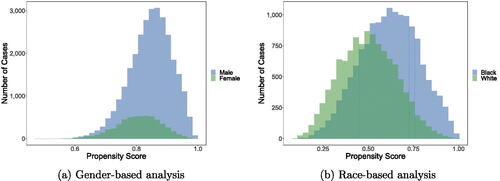
We now apply the statistical framework developed above to assess possible race and gender discrimination in real-world prosecutorial charging decisions. We start with the set of individuals in a major U.S. county who were arrested for a felony offense between 2013 and 2019. For our race-based analysis, we then limit to the 25,918 instances in which the race of the arrested individual was identified as either Black (14,686) or non-Hispanic white (11,232), and for our gender-based analysis we limit to the 34,871 instances in which the gender of the arrested individual was recorded as either male (29,283) or female (5588).¹⁶

Our dataset includes a variety of information about each case, including the criminal history of the arrested individual; the alleged offenses (e.g., burglary); the location, date, and time of the incident; whether there is body-worn camera footage; whether a weapon was involved; whether an elderly victim was involved; and whether there was gang involvement. (See Appendix D for additional details.) We also know the ultimate charging decision for each case. Disaggregating by gender, 51% of cases involving a male arrestee were charged, compared to 45% of cases involving a female arrestee; and disaggregating by race, 51% of cases involving a Black arrestee were charged, compared to 50% of cases involving a white arrestee.

To gauge the extent to which charging decisions may suffer from disparate treatment by race or gender, we estimate the sate ${}_M$. We start by checking that overlap is satisfied for both our race-based and our gender-based analyses. Recall that overlap means $\mathrm{Pr}(Z=z | X=x,M=1)>0$, where Z = 1 indicates an individual’s “treatment” status (i.e., whether an individual is male in our analysis of gender discrimination, or Black in our analysis of racial discrimination), X is a vector of observed case features, and M = 1 means we restrict to those individuals who were arrested. In contrast to ignorability, overlap can be assessed directly by examining the data. To do so, we estimate propensity scores (Rosenbaum and Rubin 1983a), $\mathrm{Pr}(Z=z | X=x,M=1)$, via an L¹-regularized (lasso) logistic regression model. In Figure 4, we plot the distribution of the estimated propensity scores. In the left panel we disaggregate by gender, and in the right panel we disaggregate by race (Black and white). In situations where overlap does not hold, it is common to restrict one’s analysis to a region of the covariate space where it does hold. In our case, however, the vast majority of the data are already far from the endpoints of the unit interval, so we work with the dataset in its entirety.

Fig. 4. We plot, for both our gender-based (left) and race-based (right) analyses, the distribution of propensity scores, disaggregated by observed treatment status. We find that the propensity scores are concentrated away from the interval endpoints, satisfying overlap.

As discussed in Section 3, regression-based estimators can be viewed as a parametric variant of the stratified difference-in-means estimator Δ_n . Thus, to help account for the high dimensionality of our feature set, we now estimate the sate ${}_M$ via linear regression. In particular, for ease of interpretation, we use a linear probability model:(14) $$\mathbb{E}[Y | Z,X]={\beta }_0+{\beta }_{1}Z+{\beta }_2^{T}X,$$(14) where Y indicates whether an arrested individual was charged, and X denotes the vector of covariates.

In the gender model, we find that the ${\widehat{\text{SATE}}}_M$—as given by ${\widehat{\beta }}_1$—is 0.025 (95% CI: [0.014, 0.037]); and in the race model, we find that the ${\widehat{\text{SATE}}}_M$ is –0.008 (95% CI: [–0.018, 0.002]). These results indicate that the charging rate for men is slightly higher than the rate for similar women, and that the charging rate for Black individuals is on par with that of similar white individuals, mirroring the patterns we saw with the raw, unadjusted charging rates. If there are no unmeasured confounders (i.e., if subset ignorability holds) and our parametric model is appropriate, these results suggest race and gender have a relatively modest impact on charging decisions in the jurisdiction we consider.

To help contextualize these results, we note that past studies have found mixed evidence of disparate treatment in prosecutorial charging decisions, likely due in part to differences in the jurisdictions and time periods analyzed, and the methods employed. In one of the most comprehensive investigations to date, Rehavi and Starr (2014) examined nearly 40,000 individuals in the federal criminal justice system from initial arrest to final sentencing. The authors found that disparate treatment in prosecutorial charging decisions—specifically for charges with statutory mandatory minimum sentences—was a primary driver for sentencing disparities between Black and white individuals. In contrast, in a recent experimental study, Robertson, Baughman, and Wright (2019) found no evidence of racial bias in charging decisions when they presented prosecutors with vignettes in which the race of the suspect was randomly varied. Similarly, in an observational analysis of prosecutors at the San Francisco District Attorney’s Office, MacDonald and Raphael (2021) found little evidence of discrimination in charging decisions—in fact, the authors found that white individuals were charged slightly more often than similarly situated Black individuals. Finally, in a recent quasi-random study of charging decisions at a large metropolitan district attorney’s office, Chohlas-Wood et al. (2021) similarly found little evidence of disparate treatment.

The AUC of our outcome model in Equation (14)(14) $$\mathbb{E}[Y | Z,X]={\beta }_0+{\beta }_{1}Z+{\beta }_2^{T}X,$$(14) —fit with all available covariates, including race and gender—is 86%, indicating that it can predict charging decisions well. Our model, however, cannot capture all aspects of prosecutorial decision making, as at least some information used by prosecutors (e.g., forensic evidence) is not recorded in our dataset, meaning that subset ignorability likely does not hold exactly. To check the robustness of our causal estimates to such unmeasured confounding, one may use a variety of statistical methods for sensitivity analysis (Rosenbaum and Rubin 1983b; Imbens 2003; McCandless, Gustafson, and Levy 2007; Carnegie, Harada, and Hill 2016; Dorie et al. 2016; McCandless and Gustafson 2017; Franks, D’Amour, and Feller 2019; Jung et al. 2020). At a high level, these methods posit relationships between the unmeasured confounder and both the treatment variable (e.g., race or gender) and the outcome (e.g., the charging decision), and then examine the sensitivity of estimates under the model of confounding.

We apply a technique for sensitivity analysis recently introduced by Cinelli and Hazlett (2020). In brief, their approach bounds the extent to which a coefficient estimate in a linear model—like ${\widehat{\beta }}_1$ in Equation (14)(14) $$\mathbb{E}[Y | Z,X]={\beta }_0+{\beta }_{1}Z+{\beta }_2^{T}X,$$(14) —might change if one were to refit the model including an unmeasured confounder U. More specifically, under the extended model$$\mathbb{E}[Y | Z,X,U]={\beta }_0+{\beta }_{1}Z+{\beta }_2^{T}X+\gamma U,$$

Cinelli and Hazlett bound the change in ${\widehat{\beta }}_1$ in terms of two partial R² values: $R_{Y\sim U\mathrm{ }|\mathrm{ }Z,X}^2$ and $R_{Z\sim U\mathrm{ }|\mathrm{ }X}^2$. These two values, respectively, quantify how much residual variance in the outcome Y and treatment Z is explained by U. Formally, $R_{Y\sim U\mathrm{ }|\mathrm{ }Z,X}^2$ is defined in terms of the R² of two linear regressions: one using all the covariates X, Z, and U to estimate Y ($R_{\text{full}}^2$), and one excluding U ($R_{\text{red}}^2$). Then, $R_{Y\sim U\mathrm{ }|\mathrm{ }Z,X}^2=(R_{\text{full}}^2-R_{\text{red}}^2)/(1-R_{\text{red}}^2)$. The quantity $R_{Z\sim U\mathrm{ }|\mathrm{ }X}^2$ is defined analogously. As these partial R² values increase, so does the amount by which ${\widehat{\beta }}_2$ could change.

The contour plots in Figure 5 show the maximum amount by which the ${\widehat{\text{SATE}}}_M$ may change as a function of $R_{Y\sim U\mathrm{ }|\mathrm{ }Z,X}^2$ and $R_{Z\sim U\mathrm{ }|\mathrm{ }X}^2$ for our analysis of gender and race—with that change potentially increasing or decreasing the estimate. The red lines trace out values for which the maximum change equals our empirical point estimates of the ${\widehat{\text{SATE}}}_M$. In particular, an unmeasured confounder lying above the red line could be sufficient to change the sign of our estimate.

Fig. 5. Contour plots describing the sensitivity of the ${\widehat{\text{SATE}}}_M$ to unmeasured confounding, for our analysis of gender (left) and race (right). The plots indicate the maximum amount the ${\widehat{\text{SATE}}}_M$ may change under the Cinelli and Hazlett (2020) model of confounding, parameterized by two partial R² values. The red curves correspond to a change equalling the magnitude of the ${\widehat{\text{SATE}}}_M$ estimated from the available data. Thus, an unobserved confounder corresponding to a point above the red curve would be capable of changing the sign of our estimate. To aid interpretation, both plots display the partial R² values associated with several observed subsets of covariates.

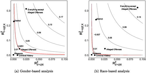
A key hurdle in sensitivity analysis is positing a reasonable range for the strength of a possible unmeasured confounder. To aid interpretation, we compute the partial R² values for various subsets of observed covariates, as recommended by Cinelli and Hazlett. For each such subset, we fit the regression model in Equation (14)(14) $$\mathbb{E}[Y | Z,X]={\beta }_0+{\beta }_{1}Z+{\beta }_2^{T}X,$$(14) both with and without that subset, which in turn yields a pair of partial R² values for that subset of covariates.

The contour plots in Figure 5 contain these reference points for five different subsets of covariates: (a) the subset describing criminal history (e.g., number of prior convictions and number of prior arrests); (b) the alleged offenses (e.g., burglary); (c) the subset of all covariates except for the alleged offenses; (d) the district in which the alleged incident took place; and (e) whether a weapon was alleged to have been used. We find that the partial R² values associated with criminal history and whether a weapon was used are below the red curves for both our analysis of gender and race, indicating that a confounder with comparable marginal explanatory power to these covariates would not be sufficient to change the sign of our estimates. However, the partial R² values corresponding to the alleged offenses and the district in which the charges were filed are near the red curve for our gender-based analysis and far above the curve for our race-based analysis, meaning that omitting a covariate with similar explanatory power could qualitatively change our conclusions. Furthermore, the partial R² values corresponding to everything except the alleged offenses are far above the red curve in both cases, suggesting that an unobserved confounder of similar strength could again substantially alter our results. For instance, in this extreme scenario, inclusion of a currently omitted confounder with similar characteristics in the race-based analysis could yield an estimated treatment effect of more than 13%.

One cannot know the exact nature and impact of unmeasured confounding. Thus, as in many applied statistical problems, we must rely in large part on domain expertise and intuition to form reasonable conclusions. In this case, given the results of our sensitivity analysis, we interpret our empirical findings as providing evidence that perceived gender and race have limited effects on prosecutorial charging decisions in the jurisdiction we consider. As with the sate ${}_M$, our sensitivity analysis is solely focused on discrimination in the charging decision, and, in particular, is not designed to capture the cumulative effects of discrimination stemming from arrests and other earlier decision points.

5 Discussion

We have outlined a formal causal framework to ground observational studies of discrimination. We specifically showed that subset ignorability, together with overlap, is sufficient to guarantee that one important causal measure of discrimination (the sate ${}_M$) is nonparametrically identified in a canonical two-stage decision-making setting. In this context, we therefore, believe potential issues of post-treatment bias are more appropriately thought of as concerns about omitted variables. Indeed, our treatment of interest—perception of race by the second decision maker—occurs after the subsetting in the first stage, and so it is not post-treatment relative to the selection process. As such, we demonstrated that a traditional regression-based analysis can be used to assess discrimination in real-world prosecutorial charging decisions, even though the underlying arrests may have been discriminatory in unknown ways. In that example—as in many applied settings—subset ignorability may only hold approximately, and our empirical analysis illustrates the importance of sensitivity analysis for robust inference.

Measurements of the sate ${}_M$ can be an important step in quantifying discrimination by specific decision makers at specific points in time. In our running example, estimates of the sate ${}_M$ can help identify prosecutors who may be making systematically biased charging decisions. Identification of bias, however, is only the first step toward reform. To mitigate identified disparities, one could imagine a variety of interventions, such as training programs (Spencer, Charbonneau, and Glaser 2016), or blinding prosecutors to the race of arrested individuals (Chohlas-Wood et al. 2021). As with all interventions, care must be taken to ensure they do not have unintended consequences. Changes in prosecutorial policies could have negative spillover, for example on policing, or unexpected equilibrium effects, such as overall harsher charging decisions.

The sate ${}_M$ is but one way to characterize and inform interventions designed to reduce discriminatory behavior. There are at least two broad notions of discrimination, which approximately map to the legal concepts of disparate treatment and disparate impact. Both involve causal interpretations, though with key differences in the definition of the estimand. Disparate treatment concerns the causal effect of race on outcomes—as we formalize here by the sate ${}_M$—with behavior often driven by animus or explicit racial categorization. Disparate impact, on the other hand, concerns the causal effect of policies or practices on unjustified racial disparities, regardless of intent. Disparate treatment and disparate impact both play important roles in legal and policy discussions, and the perspective one adopts in any given situation affects the choice of statistical estimation strategy and the interpretation of results (Jung et al. 2018).

We have throughout focused on the statistical foundations and measurement of disparate treatment. In our primary example, we estimate—assuming subset ignorability holds—that perceived race and gender have relatively small effects on prosecutorial charging decisions in the jurisdiction we examine. We further demonstrate that these estimates are moderately robust to potential omitted-variable bias. However, that finding, in and of itself, does not mean charging decisions are equitable in a broader sense. Consider, for example, the 1637 cases in our data involving alleged possession of controlled substances by Black or non-Hispanic white individuals. Of these, 748 cases (46%) were ultimately charged, and charging rates by race were nearly identical across race groups, offering little prima facie evidence of disparate treatment. However, among the 748 charged cases, 464 (62%) involved a Black individual—far exceeding the proportion of Black residents in the county we study. Charging decisions for these cases thus impose a heavy burden on Black individuals, even if those decisions were not tainted by animus. To the extent that prosecution of drug crimes is misaligned with community goals, these decisions create an unjustified, and discriminatory, disparate impact.

Rigorously estimating discrimination is a daunting task that requires careful consideration. At an empirical level, it is often difficult to obtain detailed data on individual decisions, in which case benchmark analysis may be inadequate—even if coupled with sensitivity analysis. At a theoretical level, we have a limited statistical language to make precise concepts such as animus and implicit bias that are central to discrimination research. Further, as we note above, past work has often framed discrimination as the causal effect of race on behavior, but other conceptions of discrimination, such as disparate impact, are equally important for assessing and reforming practices. Finally, the conclusions of discrimination studies are generally limited to specific decisions that happen within a long chain of potentially discriminatory actions. Quantifying discrimination at any one point (e.g., in charging decisions) does not yield estimates of specific or cumulative discrimination at other points (e.g., in arrest decisions). Despite these important considerations, we hope our work helps place discrimination research on more solid statistical footing, and provokes further interest in the subtle conceptual and methodological issues at the heart of discrimination studies.

Acknowledgments

We thank Alex Chohlas-Wood, Avi Feller, Andrew Gelman, Zhiyuan “Jerry” Lin, Julian Nyarko, Brendan O’Flaherty, Elizabeth Ogburn, José Luis Montiel Olea, Steven Raphael, James Robins, Rajiv Sethi, Amy Shoemaker, and Ilya Shpitser for helpful conversations. Code to replicate our analysis is available online at: https://github.com/stanford-policylab/gcbsgh-rep.

Notes

1 There are some differences between the idealized audit study described above and these two experiments. Chohlas-Wood et al. conduct a quasi-random field trial in which they mask—but do not switch—the stated race of individuals in police narratives used to make actual charging decisions. Robertson, Baughman, and Wright survey prosecutors in a randomized lab experiment and ask them, hypothetically, what their charging decision would be based on fact patterns in which the race of the suspect is manipulated. Although neither of these studies maps exactly to the hypothetical experiment motivating our estimand, both demonstrate the feasibility of conducting such an experiment.

2 It suffices to compare groups of cases that have the same distribution of potential outcomes—even if the cases themselves are not identical—a property we formalize in Definition 2 below.

3 To avoid imagining values of Z for individuals not arrested, one could also make them “missing” by setting $Z=Z(D,M),Z(d,0)=\text{NA},Z(d,1)=d$, $Y(\text{NA},1)=\text{NA}$, and $Y(z,0)=0$ for $z\in \{w,b,\text{NA}\}$, as we do in the simulation in Section 3. This does not affect any of the mathematical details in what follows.

4 ⁴ The sate ${}_M$ is notationally equivalent to the cde ${}_{M=1}$ defined in Knox, Lowe, and Mummolo (2020). In our case, however, we have taken care to specify that the first parameter in the quantity Y(z, m) denotes intervening on the second-stage perception of race. Moreover, the sate ${}_M$ is distinct from what Knox, Lowe, and Mummolo call the ate ${}_{M=1}$.

5 In the following, we assume that X is discrete for simplicity of exposition; for continuous analogues of these results, see Appendix C.

6 See Heckman (1979) for related discussion on interpreting sample selection bias as omitted-variable bias.

7 To be explicit, our point is that the original te and the new sate ${}_M$ are the same quantities, and hence, are estimable using the same data. However, the new sate ${}_M$ (which subsets on individuals who are stopped among those who are spotted) and the original sate ${}_M$ (which subsets on individuals who are arrested among those who are stopped), are, in contrast, not equal in general, and not necessarily estimable using the same data. In particular, if one wants to estimate either the original te or, equivalently, the new sate ${}_M$, the arrest decision can be viewed as an intermediate variable, and, accordingly, subsetting to arrested individuals would in general introduce post-treatment bias.

8 The formalism above shows a certain statistical equivalence between estimands having different starting points of the decision-making process. Nonetheless, the choice of starting point corresponds to measuring discrimination across different parts of the process, and so different estimands are relevant in different contexts. As such, we do not assert any normative ordering among them.

9 Importantly, even if the population of individuals spotted by police at a street corner is a (near) random sample of people living or working in the neighborhood, we still cannot think of race as being randomly assigned in that subset. In particular, spotted individuals may still differ on a variety of dimensions (e.g., socio-economic status) across race groups. As such, one would need to statistically account for these differences in any analysis that seeks to measure disparate treatment.

10 ¹⁰ In the case of biological sex, one might consider assignment to occur at conception, though that is typically not the primary moment of interest in studies of sex discrimination.

11 ¹¹ In particular, we follow Pearl (2009) in representing unobserved confounding by bidirectional dashed arrows; see Section 1.2.1. We do deviate from Pearl in one aspect of our notation: we write counterfactuals as Y(z, m) instead of $Y_{z,m}(u)$, suppressing the notational dependence on u. The former notation aligns with the popular Rubin-Neyman potential outcome notation that we use when defining the sate ${}_M$. We further note that this SEM is included primarily for illustrative purposes, and consequently contains some simplifications, such as strictly binary covariates. In practice, we recommend reasoning about subset ignorability and its relevant potential outcomes directly.

12 Because Z and D are separately manipulable in our framing, this quantity—obtained by first subsetting on arrested individuals, and then computing the average difference between potential outcomes—can also be expressed in the do-calculus: sate ${}_M=\mathbb{E}[Y | do(Z=b),M=1]-\mathbb{E}[Y | do(Z=w),M=1]$. However, as is common in causal mediation analysis, if there were only one indecomposable treatment (e.g., if one instead imagined directly manipulating S) then the corresponding estimand could no longer be expressed using do-operations alone (Pearl 2009, 2015).

13 In general, first-stage discrimination such as discriminatory arrest decisions or fabrication of evidence in arrest reports does not affect the consistency of the stratified difference-in-means estimator, since subset ignorability will continue to hold. Consistency may fail if discrimination is so extreme that overlap fails, for example, if no white people are arrested.

14 In the prosecutorial context, sufficiently diligent data gathering can mitigate this possibility; many offices maintain detailed case files, and we make use of such records in our empirical analysis in Section 4. In general studies of discrimination, it is important to ensure that decision factors are accurately captured and made available to analysts.

15 More specifically, the full set of parameters in our simulation was set as follows: ${\mu }_L=0.3,{\mu }_X=0.3,{\mu }_A=0.3,\delta =0.1,\gamma =-0.1,{\alpha }_0=0.1,{\alpha }_A=0.3,{\alpha }_{\text{black}}\in \{0.2,0.25,0.3,0.35,0.4\}$, ${\lambda }_0=0.2,{\lambda }_A=0.6,{\lambda }_{\text{black}}=0.1,{\beta }_0=0.2,{\beta }_X=0.4,{\beta }_R=0.2$, and ${\beta }_{\text{black}}\in \{0.2,0.25,0.3,0.35,0.4\}$.

16 Both Hispanic and non-Hispanic white individuals in our dataset appear to have been recorded simply as “white.” To disentangle these two categories, we followed past work and imputed Hispanic ethnicity from surnames (Word and Perkins 1996; Word et al. 2008; Pierson et al. 2020).

17 As noted in Footnote 12 above, since we have restricted to the context of a single treatment Z, many of the quantities we consider are not expressible via the do-calculus, though they are still expressible in terms of potential outcomes. We emphasize that these potential outcomes should be understood in the conventional sense (Pearl 2009): $Y(z,1)$ represents what would have resulted for an individual if, counterfactually, one had intervened on M so that M = 1 and Z so that Z = z. Although directly manipulating the first-stage decision so that M = 1 may be implausible in some situations—for instance, it may be challenging in practice to intervene on an arresting officer’s decision—no issue arises in our setting as we are only concerned with the outcomes $Y(z,1)$ for individuals who would be arrested in the absence of such an intervention (i.e., where it is already the case that M = 1). Moreover, while the FFRCISTG framework (Robins 1986; Richardson and Robins 2013) may consider these to be “cross-world” counterfactual quantities, we note that recent extensions of these frameworks discussed in Robins, Richardson, and Shpitser (2020) could accommodate our estimand and identifying assumptions by allowing for the race variable to be split into race variables that are time- and context-specific, as we did in the main body of the article.

18 The pushforward measure ${\mu }_{X\mathrm{ }|\mathrm{ }M=1}$ is the measure on $\mathcal{X}$—the range of X—given by ${\mu }_{X\mathrm{ }|\mathrm{ }M=1}[A]=\mathrm{Pr}(X\in A | M=1)$ for measurable $A\subseteq \mathcal{X}$.

19 To see this, first note that, in general, $\mathbb{E}[Y | Z=z,X=x,M=1]$ is uniquely defined up to a set of measure zero with respect to the pushforward measure ${\mu }_{Z,X\mathrm{ }|\mathrm{ }M=1}$. Now, for fixed z, suppose, toward a contradiction, that $f_1(x)$ and $f_2(x)$ are two versions of $\mathbb{E}[Y | Z=z,X=x,M=1]$ that differ on a set A such that $\mathrm{Pr}(X\in A | M=1)>0$. Then, by the generalized overlap condition, $\mathrm{Pr}(Z=z,X\in A | M=1)={\int }_A\mathrm{Pr}(Z=z | X=x,M=1) \mathrm{d}{F}_{X\mathrm{ }|\mathrm{ }M=1}>0$, contradicting the fact that $f_1(x)\ne f_2(x)$ only on a null set with respect to the pushforward measure ${\mu }_{Z,X\mathrm{ }|\mathrm{ }M=1}$.

Appendix A:

A Comparison to Alternative Ignorability Conditions

To better understand subset ignorability, we compare it to alternative conditions that recently have been proposed in the context of discrimination studies. In particular, we compare subset ignorability to a set of assumptions introduced by Knox, Lowe, and Mummolo (2020), which they call treatment ignorability, mediator ignorability, and mediator monotonicity. We show that this set of assumptions, like subset ignorability, is sufficient—but not necessary—to ensure the sate ${}_M$ is nonparametrically identified by data on second-stage decisions. Importantly, however, the Knox, Lowe, and Mummolo conditions are unlikely to be satisfied in important examples of potentially discriminatory decision making where subset ignorability holds (either exactly or approximately) and the sate ${}_M$ accordingly can be estimated, like those situations presented in Sections 3 and 4.

Aside from the Knox, Lowe, and Mummolo conditions, it is instructive to compare subset ignorability to sequential ignorability (Imai, Keele, and Tingley 2010a; Imai, Keele, and Yamamoto 2010b), a popular and often useful concept that was introduced to formalize causal mediation analysis, and one that is closely related to the Knox, Lowe, and Mummolo conditions. Sequential ignorability is strictly stronger than subset ignorability, meaning that the former implies the latter but that the converse does not hold. In the setting of discrimination studies, there is little reason to believe sequential ignorability—or reasonable approximations of it—would be satisfied, and we primarily discuss the idea to clarify its distinction from subset ignorability.

The alternative ignorability conditions considered here were developed in the context of a single treatment. Therefore, to facilitate a direct comparison between subset ignorability and these alternatives, we adopt this single-treatment perspective throughout the Appendix. As discussed in the main text, there are substantive issues with positing a single manipulation of (perceived) race, gender, or other immutable characteristics in many multi-stage settings. Formally, however, it is straightforward to collapse Z and D to a single treatment—which we call Z—that affects both the first-stage and the second-stage decisions. In particular, we now assume the potential outcomes M(z) and Y(z, m) satisfy the consistency relations $M=M(Z)$ and $Y=Y(Z,M)$. We emphasize that in this new framing, the definition of subset ignorability in Equation (4)(4) $$Y(z,1)\perp \text{}\perp Z | X,M=1$$(4) remains the same and that Theorem 1 likewise holds unaltered—since neither explicitly references the first-stage potential outcomes.17

We start by formally considering sequential ignorability, following Imai, Keele, and Tingley (2010a); Imai, Keele, and Yamamoto (2010b).

Definition A.

1 (Sequential ignorability). We say that sequential ignorability is satisfied when the following two conditional independence criteria hold:(A.1) $$\{Y(z\prime ,m),M(z)\}\perp \text{}\perp Z | X,$$(A.1) (A.2) $$Y(z\prime ,m)\perp \text{}\perp M | Z,X,$$(A.2) for $z,z\prime \in \{w,b\}$ and $m\in \{0,1\}$.

The two key conditional independence assumptions we list are the same as in the definition of sequential ignorability given by Imai, Keele, and Tingley (2010a); Imai, Keele, and Yamamoto (2010b), but to facilitate direct comparison with other ignorability criteria, we omit from our definition the accompanying overlap conditions. Also, for ease of exposition, we present the definition in the setting of binary treatment and mediator variables, though the original was more general. In the context of our running example, sequential ignorability means that: (a) conditional on the observed covariates X, the potential outcomes for charging Y(z, m) and arrest M(z) are jointly independent of an individual’s actual race Z; and (b) conditional on the observed covariates X and an individual’s race Z, the arrest decision M is independent of the potential charging outcomes Y(z, m).

Theorem A.

1, below, shows that sequential ignorability implies subset ignorability, but also, importantly, that sequential ignorability is a strictly stronger condition. To understand why, consider the stylized model of Section 3.1, in which one has all of the information that drives a prosecutor’s charging decision—satisfying subset ignorability—but not all of the information that drives an officer’s arrest decision. For example, suppose the prosecutor has access to the officer’s report, but not the arrested individual’s actual behavior. In this case, one would in general expect the first condition of sequential ignorability—in Equation (A.1)(A.1) $$\{Y(z\prime ,m),M(z)\}\perp \text{}\perp Z | X,$$(A.1) —to be violated. In particular, without detailed data on what an officer observes, there is little reason to think the arrest potential outcomes, M(z), would be independent of an individual’s race, even controlling for factors available to the prosecutor.

We next formally present the definitions of treatment ignorability, mediator ignorability, and mediator monotonicity proposed by Knox, Lowe, and Mummolo, starting with treatment ignorability.

Definition A.

2 (Treatment ignorability). Treatment ignorability is the combination of the following two conditional independence criteria: for $z,z\prime \in \{w,b\}$ and $m\in \{0,1\}$,(A.3) $$M(z)\perp \text{}\perp Z | X,$$(A.3) (A.4) $$Y(z\prime ,m)\perp \text{}\perp Z | M(w),M(b),X.$$(A.4)

In the context of arrest and charging decisions, treatment ignorability means that: (a) the potential outcomes for the arrest decision M(z) are independent of race Z, after conditioning on the observed covariates X; and (b) the potential outcomes for the charging decision $Y(z\prime ,m)$ are independent of race Z after conditioning on both the covariates X and the arrest potential outcomes M(w) and M(b).

The first condition of treatment ignorability is similar to the first condition of sequential ignorability, and it is unlikely to hold in our setting for the same reason. In general, given only information about what motivates the second-stage decision (e.g., charging, in our case) one cannot say much about what occurs in the first stage (e.g., arrest). But, critically, such information about the first stage is not necessary to estimate the sate ${}_M$, which only quantifies discrimination in the second-stage decision. Theorem 1 makes that statement precise, showing that subset ignorability—which does not consider first-stage potential outcomes—is sufficient to ensure the sate ${}_M$ is nonparametrically identified by the second-stage data.

The second criterion of treatment ignorability appears similar in spirit to subset ignorability, but it conditions on the potential outcomes M(w) and M(b) rather than on the actual outcome M. In practice, that distinction may not be too significant; in theory, however, the difference between the two is large. As we show in Theorem A.1 below, treatment ignorability alone—even with its strong assumption on the first stage—is not sufficient to ensure the sate ${}_M$ is identified by the second-stage data.

Finally, we consider mediator ignorability and the related mediator monotonicity condition.

Definition A.

3 (Mediator ignorability). For $z\in \{w,b\}$ and $m\in \{0,1\}$, mediator ignorability is satisfied when(A.5) $$Y(z,m)\perp \text{}\perp M(w) | Z=z,M(b)=1,X.$$(A.5)

Definition A.

4 (Mediator monotonicity). Mediator monotonicity is satisfied when(A.6) $$M(b)\ge M(w).$$(A.6)

In our running example, mediator ignorability means that the charging potential outcomes Y(z, m) are independent of one of the arrest potential outcomes—M(w), the arrest decision for (counterfactually) white individuals—conditional on the observed covariates X, and among individuals of race Z = z, who would be arrested if they were Black. The asymmetry in this condition stems from the additional mediator monotonicity constraint considered by Knox, Lowe, and Mummolo: $M(b)\ge M(w)$, meaning that an individual who would be arrested if white would also be arrested if Black. The monotonicity condition is perhaps intuitively plausible given our understanding of racial discrimination, but the conditional independence assumption of mediator ignorability appears harder to interpret.

Having introduced the key definitions, we now present our main analytic result, Theorem A.1, which summarizes and formalizes our discussion of the various ignorability assumptions and their connections to estimating discrimination. In particular, we show that sequential ignorability is a strictly stronger assumption than subset ignorability, and recapitulate (from Theorem 1) that subset ignorability is a sufficient condition for the difference-in-means estimator Δ_n to yield consistent estimates of the sate ${}_M$. Further, we show that treatment ignorability is not a necessary condition for Δ_n to yield consistent estimates. We show this by explicitly constructing examples for which ${\Delta }_n\stackrel{\mathrm{a}.\mathrm{s}.}{\to }{\mathrm{ }\text{SATE}}_M$, but which violate the treatment ignorability condition. We additionally show that treatment ignorability is not a sufficient condition to guarantee consistency, despite its formal resemblance to the (sufficient) subset ignorability condition. To do so, we construct a family of observationally equivalent examples that satisfy treatment ignorability but which have different values of the sate ${}_M$. Accordingly, no estimator, including Δ_n , can yield a consistent estimate of the sate ${}_M$ for every instance in the family. Importantly, the more conventional assumption of subset ignorability is sufficient to ensure the sate ${}_M$ can be identified from data on the second-stage decisions.

Theorem A.1.

Assume overlap holds, meaning that $\mathrm{Pr}(Z=z | X=x,M=1)>0$ for all x and z. Then we have the following collection of implications and nonimplications

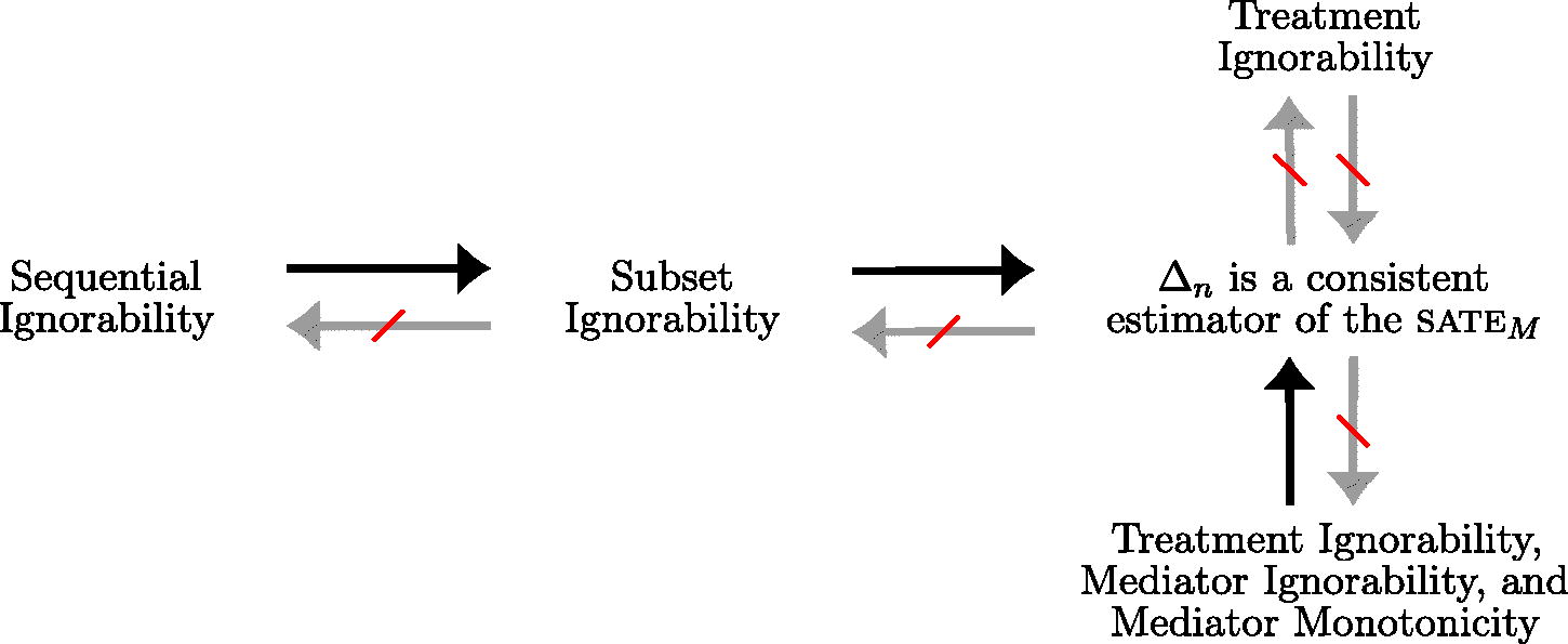
Proof.

Theorem 1 shows that subset ignorability implies that Δ_n is a consistent estimator of the sate${}_M$. We show the remaining seven implications and nonimplications in turn, starting with the claim that sequential ignorability implies subset ignorability. In particular, we prove that the conjunction of treatment ignorability, mediator ignorability, and mediator monotonicity implies that Δ_n is a consistent estimator of the sate${}_M$—a fact initially suggested by Knox, Lowe, and Mummolo

Case 1

(Sequential ignorability implies subset ignorability). The first condition of sequential ignorability, in Equation (A.1)(A.1) $$\{Y(z\prime ,m),M(z)\}\perp \text{}\perp Z | X,$$(A.1) , states that Y(z, m) and $M(z\prime )$ are jointly independent of Z given X: $\{Y(z,m),M(z\prime )\}\perp \text{}\perp Z | X$. From this, it immediately follows that Y(z, m) alone is independent of Z given X: $Y(z,m)\perp \text{}\perp Z | X$. Now, because $Y(z,m)\perp \text{}\perp M | Z,X$—which is the second condition of sequential ignorability, in Equation (A.2)(A.2) $$Y(z\prime ,m)\perp \text{}\perp M | Z,X,$$(A.2) —we have that $Y(z,m)\perp \text{}\perp \{Z,M\} | X$, by the contraction property of conditional independence. Therefore, by the weak-union property,(A.7) $$Y(z,m)\perp \text{}\perp Z | M,X.$$(A.7)

Subset ignorability now follows, as it is the special case in which M = 1 in Equation (A.7)(A.7) $$Y(z,m)\perp \text{}\perp Z | M,X.$$(A.7) .

Case 2

(Subset ignorability does not imply sequential ignorability). Sequential ignorability is an intuitively stronger condition than subset ignorability, as the former requires that Z is independent of the mediator potential outcomes M(z) given X. Indeed, the synthetic example given in Section 3 satisfies subset ignorability but violates sequential ignorability.

To formally establish our claim, we construct an even simpler example that satisfies subset ignorability but not sequential ignorability. First, suppose that $Y(z,1)=1$ and $Y(z,0)=0$, deterministically for $z\in \{b,w\}$. In particular, using the language of our policing and prosecution application, everyone who is arrested is charged, regardless of race. We further set X = 1, which effectively means that there are no contextual variables. Finally, we set(A.8) $$\begin{array}{cc}\mathrm{Pr}\hfill & (Z=z,M(b)=m_b,M(w)=m_w)\hfill \\ \hfill & =\mathrm{Pr}(Z=z)·\mathrm{Pr}(M(b)=m_b|Z=z)\hfill \\ \hfill & ·\mathrm{Pr}(M(w)=m_w|Z=z),\hfill \end{array}$$(A.8) where $\mathrm{Pr}(Z=z)=\frac{1}{2},\mathrm{Pr}(M(z)=1 | Z=w)=\frac{1}{2}$, and $\mathrm{Pr}(M(z)=1 | Z=b)=1$. Note that $M=M(Z)$ and $Y=Y(Z,M)$, and so the above description fully defines the joint distribution on all the relevant variables.

Now, because $Y(z,1)$ = 1, we trivially have that $Y(z,1)\perp \text{}\perp Z | M$, meaning that subset ignorability is satisfied. But, because $M(z)\cancel{\perp \text{}\perp }Z$, sequential ignorability is violated.

Case 3

(Consistency of Δ_n does not imply subset ignorability holds). At a high level, even if the potential outcomes $Y(z,1)$ are not independant of Z—violating subset ignorability—Δ_n can still be a consistent estimator when there is appropriate cancelation. For a concrete illustration of this in the context of our two-stage arrest and charging application, consider a simple example in which: (a) there are no contextual variables (i.e., X = 1); (b) the population is evenly split across race groups (i.e., $\mathrm{Pr}(Z=z)=\frac{1}{2}$); (c) everyone in the population is arrested (i.e., M = 1); and (d) the prosecutor’s potential decisions depend on an arrestee’s actual race. Specifically, we set $Y(z,0)=0$ and $Y(z,1)$ to be a Bernoulli random variable distributed as follows:(A.9) $$\mathrm{Pr}(Y(z,1)=1 | Z)=\{\begin{array}{cc}1\hfill & z=b\wedge Z=b,\hfill \\ 0\hfill & z=w\wedge Z=b,\hfill \\ \frac{1}{2}\hfill & Z=w.\hfill \end{array}$$(A.9)

Because $Y=Y(Z,M)$, the above relationships completely specify the joint distribution of Y, Z, M, and X.

Subset ignorability is violated in this example since, by Equation (A.9)(A.9) $$\mathrm{Pr}(Y(z,1)=1 | Z)=\{\begin{array}{cc}1\hfill & z=b\wedge Z=b,\hfill \\ 0\hfill & z=w\wedge Z=b,\hfill \\ \frac{1}{2}\hfill & Z=w.\hfill \end{array}$$(A.9) , $Y(z,1)\cancel{\perp \text{}\perp }Z$. (Because X and M are constant, we need not condition on them when considering the subset ignorability criterion.) We further have,$$\begin{array}{cc}{\text{SATE}}_M\hfill & =\mathbb{E}[Y(b,1) | M=1]-\mathbb{E}[Y(w,1) | M=1]\hfill \\ \hfill & =\left(\mathbb{E}[Y(b,1) | Z=b]-\mathbb{E}[Y(w,1) | Z=b]\right)·\mathrm{Pr}(Z=b)\hfill \\ \hfill & +\left(\mathbb{E}[Y(b,1) | Z=w]-\mathbb{E}[Y(w,1) | Z=w]\right)·\mathrm{Pr}(Z=w)\hfill \\ \hfill & =\left(1-0\right)·\frac{1}{2}+\left(\frac{1}{2}-\frac{1}{2}\right)·\frac{1}{2}\hfill \\ \hfill & =\frac{1}{2}.\hfill \end{array}$$

Finally,$$\begin{array}{cc}\underset{n\to \infty }{\lim }{\Delta }_n\hfill & \stackrel{\mathrm{a}.\mathrm{s}.}{=}\mathbb{E}[Y | Z=b,M=1]-\mathbb{E}[Y | Z=w,M=1]\hfill \\ \hfill & =1-\frac{1}{2}\hfill \\ \hfill & ={\mathrm{ }\text{SATE}}_M.\hfill \end{array}$$

Thus, even though subset ignorability is violated in this example, Δ_n yields a consistent estimate of the sate ${}_M$.

Case 4

(Consistency of Δ_n does not imply treatment ignorability holds). Consider the example described in Case 2. As discussed there, subset ignorability is satisfied in that example and so, by Theorem 1, Δ_n is a consistent estimator of the sate${}_M$. However, that example does not satisfy treatment ignorability, as $M(z)\cancel{\perp \text{}\perp }Z$, contrary to Equation (A.3)(A.3) $$M(z)\perp \text{}\perp Z | X,$$(A.3) . (Because X is constant, we need not condition on it when evaluating the treatment ignorability criterion.)

Case 5

(Consistency of Δ_n does not imply that treatment ignorability, mediator ignorability, and mediator monotonicity hold). This is directly implied by Case 4.

Case 6

(Treatment ignorability does not imply Δ_n is a consistent estimator of the sate${}_M$). We show, more generally, that the sate${}_M$ is not identifiable under treatment ignorability alone. To do so, we construct a family of observationally equivalent examples that satisfy treatment ignorability but which have different values of sate${}_M$. As a result, no estimator—including Δ_n —can consistently estimate the sate${}_M$ for every example in this family.

We construct the family of examples as follows. First, as in the other cases, we set X = 1, so that there are effectively no contextual variables, and we set $Y(z,0)=0$, meaning that if an individual were not arrested, that individual could not be charged. Second, we set M(b) = 1, meaning that everyone in the population would be arrested if they were Black. Finally, we set(A.10) $$\begin{array}{cc}\mathrm{Pr}\hfill & (Y(z,1)=y_{zm},M(w)=m_w,Z=z)\hfill \\ \hfill & =\mathrm{Pr}(Y(z,1)=y_{zm}|M(w)=m_w)\hfill \\ \hfill & ·\mathrm{Pr}(M(w)=m_w)·\mathrm{Pr}(Z=z),\hfill \end{array}$$(A.10) where $\mathrm{Pr}(Z=z)=\frac{1}{2},\mathrm{Pr}(M(w)=m_w)=\frac{1}{2}$, and, for $\alpha \in [0,1]$,(A.11) $$\mathrm{Pr}(Y(z,1)=1 | M(w))=\{\begin{array}{cc}\alpha \hfill & M(w)=0\wedge z=w,\hfill \\ 1\hfill & \text{otherwise}.\hfill \end{array}$$(A.11)

The examples we construct thus, differ only in the choice of α.

Now, regardless of α, these examples all satisfy treatment ignorability. To see this, note that $M(w)\perp \text{}\perp Z$ by Equation (A.10)(A.10) $$\begin{array}{cc}\mathrm{Pr}\hfill & (Y(z,1)=y_{zm},M(w)=m_w,Z=z)\hfill \\ \hfill & =\mathrm{Pr}(Y(z,1)=y_{zm}|M(w)=m_w)\hfill \\ \hfill & ·\mathrm{Pr}(M(w)=m_w)·\mathrm{Pr}(Z=z),\hfill \end{array}$$(A.10) and $M(b)\perp \text{}\perp Z$ since M(b) is constant. Consequently, the first condition of treatment ignorability is satisfied. Equation (A.10)(A.10) $$\begin{array}{cc}\mathrm{Pr}\hfill & (Y(z,1)=y_{zm},M(w)=m_w,Z=z)\hfill \\ \hfill & =\mathrm{Pr}(Y(z,1)=y_{zm}|M(w)=m_w)\hfill \\ \hfill & ·\mathrm{Pr}(M(w)=m_w)·\mathrm{Pr}(Z=z),\hfill \end{array}$$(A.10) further implies that $Y(z,1)\perp \text{}\perp Z | M(w)$ and, since $Y(z,0)$ is constant, $Y(z,0)\perp \text{}\perp Z | M(w)$, establishing the second condition of treatment ignorability. (Because M(b) and X are constant, we need not condition on them when considering the two treatment ignorability conditions.)

We next show that all these examples are observationally equivalent. Intuitively, observational equivalence stems from the fact that the only difference between the examples is in the distribution of $Y(w,1)$ for those individuals with M(w) = 0. But for those with M(w) = 0, who would not be arrested if they were white, we never observe $Y(w,1)$.

Now, to rigorously establish observational equivalence, we must show that $\mathrm{Pr}(X=x,Y=y,Z=z | M=1)$ does not depend on the value of α. Because X is constant, we need only consider $\mathrm{Pr}(Y=y,Z=z | M=1)$. First, observe that$$\begin{array}{cc}\mathrm{Pr}(M=1)\hfill & =\mathrm{Pr}(M(w)=1,Z=w)+\mathrm{Pr}(M(b)=1,Z=b)\hfill \\ \hfill & =\mathrm{Pr}(M(w)=1)·\mathrm{Pr}(Z=w)+\mathrm{Pr}(Z=b)\hfill \\ \hfill & =\frac{3}{4}.\hfill \end{array}$$

Further, note that$$\mathrm{Pr}(Y=y,Z=z,M=1)=\mathrm{Pr}(Y(z,1)=y,Z=z,M(z)=1),$$and consider the case z = b. Then, because $Y(b,1)=1$ and M(b) = 1,(A.12) $$\mathrm{Pr}(Y=y,Z=b,M=1)=\{\begin{array}{cc}0\hfill & y=0,\hfill \\ \frac{1}{2}\hfill & y=1.\hfill \end{array}$$(A.12)

Now consider the case z = w. By Equation (A.10)(A.10) $$\begin{array}{cc}\mathrm{Pr}\hfill & (Y(z,1)=y_{zm},M(w)=m_w,Z=z)\hfill \\ \hfill & =\mathrm{Pr}(Y(z,1)=y_{zm}|M(w)=m_w)\hfill \\ \hfill & ·\mathrm{Pr}(M(w)=m_w)·\mathrm{Pr}(Z=z),\hfill \end{array}$$(A.10) ,$$\begin{array}{cc}\mathrm{Pr}(Y\hfill & (w,1)=y,Z=w,M(w)=1)\hfill \\ \hfill & =\mathrm{Pr}(Y(w,1)=y | M(w)=1)·\mathrm{Pr}(M(w)=1)·\mathrm{Pr}(Z=w)\hfill \\ \hfill & =\mathrm{Pr}(Y(w,1)=y | M(w)=1)·\frac{1}{4}.\hfill \end{array}$$

By Equation (A.11)(A.11) $$\mathrm{Pr}(Y(z,1)=1 | M(w))=\{\begin{array}{cc}\alpha \hfill & M(w)=0\wedge z=w,\hfill \\ 1\hfill & \text{otherwise}.\hfill \end{array}$$(A.11) , $\mathrm{Pr}(Y(w,1)=1 | M(w)=1)=1$, and so,(A.13) $$\mathrm{Pr}(Y=y,Z=w,M=1)=\{\begin{array}{cc}0\hfill & y=0,\hfill \\ \frac{1}{4}\hfill & y=1.\hfill \end{array}$$(A.13)

Finally, combining Equations (A.12)(A.12) $$\mathrm{Pr}(Y=y,Z=b,M=1)=\{\begin{array}{cc}0\hfill & y=0,\hfill \\ \frac{1}{2}\hfill & y=1.\hfill \end{array}$$(A.12) and (A.13) with the fact that $\mathrm{Pr}(M=1)=\frac{3}{4}$, we have$$\mathrm{Pr}(Y=y,Z=z | M=1)=\{\begin{array}{cc}0\hfill & y=0,\hfill \\ \frac{2}{3}\hfill & y=1\wedge z=b,\hfill \\ \frac{1}{3}\hfill & y=1\wedge z=w.\hfill \end{array}$$

In particular, $\mathrm{Pr}(Y=y,Z=z | M=1)$ does not depend on α, and so the examples are all observationally equivalent.

We conclude the proof by showing that the sate ${}_M$ differs across these examples. First, it remains to calculate $\mathrm{Pr}(M(w)=m_w | M=1)$. To do so, note that$$\begin{array}{cc}\mathrm{Pr}(M(w)=1,M=1)\hfill & =\mathrm{Pr}(M(w)=1,Z=w)\hfill \\ \hfill & \hspace{1em}+\mathrm{Pr}(M(w)=1,M(b)=1,Z=b)\hfill \\ \hfill & =\mathrm{Pr}(M(w)=1)·\mathrm{Pr}(Z=w)\hfill \\ \hfill & \hspace{1em}+\mathrm{Pr}(M(w)=1)·\mathrm{Pr}(M(b)=1)·\mathrm{Pr}(Z=b)\hfill \\ \hfill & =\frac{1}{2}·\frac{1}{2}+\frac{1}{2}·1·\frac{1}{2}\hfill \\ \hfill & =\frac{1}{2},\hfill \end{array}$$and so, since $\mathrm{Pr}(M=1)=\frac{3}{4}$, it follows that $\mathrm{Pr}(M(w)=1 | M=1)=\frac{2}{3}$.

Consequently, we have$$\begin{array}{cc}{\mathrm{ }\text{SATE}}_M\hfill & =\mathbb{E}[Y(b,1) | M=1]-\mathbb{E}[Y(w,1) | M=1]\hfill \\ \hfill & =\mathrm{Pr}(M(w)=1 | M=1)\hfill \\ \hfill & \hspace{1em}·(\mathbb{E}[Y(b,1) | M(w)=1,M=1]\hfill \\ \hfill & \hspace{1em}-\mathbb{E}[Y(w,1) | M(w)=1,M=1])+\mathrm{Pr}(M(w)=0 | M=1)\hfill \\ \hfill & \hspace{1em}·(\mathbb{E}[Y(b,1) | M(w)=0,M=1]\hfill \\ \hfill & \hspace{1em}-\mathbb{E}[Y(w,1) | M(w)=0,M=1])\hfill \\ \hfill & =\frac{2}{3}·(1-1)+\frac{1}{3}·(1-\mathbb{E}[Y(w,1) | M(w)=0,Z=b])\hfill \\ \hfill & =\frac{1-\alpha }{3},\hfill \end{array}$$where second to last equality follows from Equation (A.11)(A.11) $$\mathrm{Pr}(Y(z,1)=1 | M(w))=\{\begin{array}{cc}\alpha \hfill & M(w)=0\wedge z=w,\hfill \\ 1\hfill & \text{otherwise}.\hfill \end{array}$$(A.11) and the fact that the event $\{M(w)=0\wedge M=1\}$ equals $\{M(w)=0\wedge Z=b\}$; the final equality also follows from Equation (A.11)(A.11) $$\mathrm{Pr}(Y(z,1)=1 | M(w))=\{\begin{array}{cc}\alpha \hfill & M(w)=0\wedge z=w,\hfill \\ 1\hfill & \text{otherwise}.\hfill \end{array}$$(A.11) , as well as the fact that $Y(z,1)\perp \text{}\perp Z | M(w)$. We have thus, constructed a family of observationally equivalent examples that satisfy treatment ignorability but which have different sate ${}_M$, implying that the sate ${}_M$ is not in general identifiable under treatment ignorability alone.

Case 7

(Treatment, mediator ignorability, and mediator monotonicity jointly imply Δ_n is a consistent estimator of the sate ${}_M$). The proof is in two pieces. First, we derive an expression for the sate${}_M$ holding X constant, and then prove the general claim.

Supposing X = x is constant, recall that by definition M = 1 if and only if M(z) = 1 where Z = z. By mediator monotonicity, $M(b)\ge M(w)$. Therefore, the event $\{M=1\}$ can be partitioned into the following two events:

• $E_1=\{M(b)=1\wedge M(w)=1\}$,

• $E_2=\{Z=b\wedge M(b)=1\wedge M(w)=0\}$.

Recall the definition of the sate ${}_M$ in Definition 1. It follows from the law of total expectation that:(A.14) $$\begin{array}{c}{\text{SATE}}_M=\mathbb{E}[Y(b,1)-Y(z,1) | M=1]\\ \begin{array}{cc}\hfill & =\mathbb{E}[Y(b,1)-Y(z,1) | E_1]·\mathrm{Pr}(E_1 | M=1)\hfill \\ \hfill & \hspace{1em}+\mathbb{E}[Y(b,1)-Y(z,1) | E_2]·\mathrm{Pr}(E_2 | M=1)\hfill \end{array}\end{array}$$(A.14)

Now, we examine each of these summands in turn. First, consider the E₁ term:$$\mathbb{E}[Y(b,1)-Y(w,1) | E_1]=\mathbb{E}[Y(b,1) | E_1]-\mathbb{E}[Y(w,1) | E_1]$$

By the definition of $E_1=\{M(b)=1\wedge M(w)=1\}$ and the second treatment ignorability condition, Equation (A.4)(A.4) $$Y(z\prime ,m)\perp \text{}\perp Z | M(w),M(b),X.$$(A.4) , we are free to condition both terms on the right hand side by levels of Z, yielding(A.15) $$\begin{array}{c}\mathbb{E}[Y(b,1) | Z=b,E_1]-\mathbb{E}[Y(w,1) | Z=w,E_1]\\ \hspace{1em}=\mathbb{E}[Y | Z=b,E_1]-\mathbb{E}[Y | Z=w,E_1],\end{array}$$(A.15) where equality follows from replacing potential outcomes by their realized values according to the definition of $Y=Y(M,Z)$.

Next, consider the E₂ term. Again,$$\mathbb{E}[Y(b,1)-Y(w,1) | E_2]=\mathbb{E}[Y(b,1) | E_2]-\mathbb{E}[Y(w,1) | E_2].$$

It follows from mediator ignorability, Equation (A.5)(A.5) $$Y(z,m)\perp \text{}\perp M(w) | Z=z,M(b)=1,X.$$(A.5) , and the definition of E₂ that$$\begin{array}{cc}\mathbb{E}[Y(w,1) | E_2]\hfill & =\mathbb{E}[Y(w,1) | Z=b,M(b)=1,M(w)=0]\hfill \\ \hfill & =\mathbb{E}[Y(w,1) | Z=b,M(b)=1,M(w)=1]\hfill \\ \hfill & =\mathbb{E}[Y(w,1) | Z=w,M(b)=1,M(w)=1],\hfill \end{array}$$where the last equality follows from treatment ignorability, Equation (A.4)(A.4) $$Y(z\prime ,m)\perp \text{}\perp Z | M(w),M(b),X.$$(A.4) . Replacing potential outcomes with their realizations, it follows that(A.16) $$\mathbb{E}[Y(b,1)-Y(w,1) | E_2]=\mathbb{E}[Y | Z=b,E_2]-\mathbb{E}[Y | Z=w,E_1].$$(A.16)

Now, we substitute Equations (A.15)(A.15) $$\begin{array}{c}\mathbb{E}[Y(b,1) | Z=b,E_1]-\mathbb{E}[Y(w,1) | Z=w,E_1]\\ \hspace{1em}=\mathbb{E}[Y | Z=b,E_1]-\mathbb{E}[Y | Z=w,E_1],\end{array}$$(A.15) and (A.16) into Equation (A.14)(A.14) $$\begin{array}{c}{\text{SATE}}_M=\mathbb{E}[Y(b,1)-Y(z,1) | M=1]\\ \begin{array}{cc}\hfill & =\mathbb{E}[Y(b,1)-Y(z,1) | E_1]·\mathrm{Pr}(E_1 | M=1)\hfill \\ \hfill & \hspace{1em}+\mathbb{E}[Y(b,1)-Y(z,1) | E_2]·\mathrm{Pr}(E_2 | M=1)\hfill \end{array}\end{array}$$(A.14) .(A.17) $$\begin{array}{c}{\text{SATE}}_M=\left(\mathbb{E}[Y | Z=b,E_1]-\mathbb{E}[Y | Z=w,E_1]\right)·\mathrm{Pr}(E_1 | M=1)\\ \hspace{1em}+\left(\mathbb{E}[Y | Z=b,E_2]-\mathbb{E}[Y | Z=w,E_1]\right)·\mathrm{Pr}(E_2 | M=1)\\ =\left(\mathbb{E}[Y | Z=b,E_1]-\mathbb{E}[Y | Z=w,M=1]\right)·\mathrm{Pr}(E_1 | M=1)\\ \hspace{1em}+\left(\mathbb{E}[Y | Z=b,E_2]-\mathbb{E}[Y | Z=w,M=1]\right)\\ \hspace{1em}·\mathrm{Pr}(E_2 | M=1)\\ =(\mathbb{E}[Y | Z=b,E_1]·\mathrm{Pr}(E_1 | M=1)+\mathbb{E}[Y | Z=b,E_2]\\ \hspace{1em}·\mathrm{Pr}(E_2 | M=1))\\ \hspace{1em}-(\mathbb{E}[Y | Z=w,M=1]·(\mathrm{Pr}(E_1 | M=1)\\ \hspace{1em}+\mathrm{Pr}(E_2 | M=1)))\\ =\mathbb{E}[Y | Z=b,M=1]-\mathbb{E}[Y | Z=w,M=1],\end{array}$$(A.17) where the second equality follows from the fact that $\{M=1\wedge Z=w\}=\{E_1\wedge Z=w\}$ by mediator monotonicity, and the last equality follows from the facts that $\{M=1\wedge Z=b\wedge E_1\}=\{Z=b\wedge E_1\}$, $\{M=1\wedge Z=b\wedge E_2\}=\{Z=b\wedge E_2\}$, and $\mathrm{Pr}(E_1 | M=1)+\mathrm{Pr}(E_2 | M=1)=1$.

Now, suppose that X is not constant. Conditioning Y, Z, and M on X = x, it follows from the law of total expectation that(A.18) $$\begin{array}{c}\mathbb{E}[Y(b,1)-Y(w,1) | M=1]\\ =\sum _x\mathbb{E}[Y(b,1)-Y(w,1) | M=1,X=x]·\mathrm{Pr}(X=x | M=1)\hspace{1em}\\ \begin{array}{cc}\hfill & =\sum _x\mathbb{E}[Y | Z=b,M=1,X=x]·\mathrm{Pr}(X=x | M=1)\hfill \\ \hfill & \hspace{1em}-\mathbb{E}[Y | Z=w,M=1,X=x]·\mathrm{Pr}(X=x | M=1),\hfill \end{array}\end{array}$$(A.18) where the second equality follows from Equation (A.17)(A.17) $$\begin{array}{c}{\text{SATE}}_M=\left(\mathbb{E}[Y | Z=b,E_1]-\mathbb{E}[Y | Z=w,E_1]\right)·\mathrm{Pr}(E_1 | M=1)\\ \hspace{1em}+\left(\mathbb{E}[Y | Z=b,E_2]-\mathbb{E}[Y | Z=w,E_1]\right)·\mathrm{Pr}(E_2 | M=1)\\ =\left(\mathbb{E}[Y | Z=b,E_1]-\mathbb{E}[Y | Z=w,M=1]\right)·\mathrm{Pr}(E_1 | M=1)\\ \hspace{1em}+\left(\mathbb{E}[Y | Z=b,E_2]-\mathbb{E}[Y | Z=w,M=1]\right)\\ \hspace{1em}·\mathrm{Pr}(E_2 | M=1)\\ =(\mathbb{E}[Y | Z=b,E_1]·\mathrm{Pr}(E_1 | M=1)+\mathbb{E}[Y | Z=b,E_2]\\ \hspace{1em}·\mathrm{Pr}(E_2 | M=1))\\ \hspace{1em}-(\mathbb{E}[Y | Z=w,M=1]·(\mathrm{Pr}(E_1 | M=1)\\ \hspace{1em}+\mathrm{Pr}(E_2 | M=1)))\\ =\mathbb{E}[Y | Z=b,M=1]-\mathbb{E}[Y | Z=w,M=1],\end{array}$$(A.17) , using the fact that X is constant on each of the events $\{X=x\}$. Equation (A.18)(A.18) $$\begin{array}{c}\mathbb{E}[Y(b,1)-Y(w,1) | M=1]\\ =\sum _x\mathbb{E}[Y(b,1)-Y(w,1) | M=1,X=x]·\mathrm{Pr}(X=x | M=1)\hspace{1em}\\ \begin{array}{cc}\hfill & =\sum _x\mathbb{E}[Y | Z=b,M=1,X=x]·\mathrm{Pr}(X=x | M=1)\hfill \\ \hfill & \hspace{1em}-\mathbb{E}[Y | Z=w,M=1,X=x]·\mathrm{Pr}(X=x | M=1),\hfill \end{array}\end{array}$$(A.18) is identical to the expression in the statement of Theorem 1, and so the estimator Δ_n converges almost surely to the quantity on the right-hand side of Equation (A.18)(A.18) $$\begin{array}{c}\mathbb{E}[Y(b,1)-Y(w,1) | M=1]\\ =\sum _x\mathbb{E}[Y(b,1)-Y(w,1) | M=1,X=x]·\mathrm{Pr}(X=x | M=1)\hspace{1em}\\ \begin{array}{cc}\hfill & =\sum _x\mathbb{E}[Y | Z=b,M=1,X=x]·\mathrm{Pr}(X=x | M=1)\hfill \\ \hfill & \hspace{1em}-\mathbb{E}[Y | Z=w,M=1,X=x]·\mathrm{Pr}(X=x | M=1),\hfill \end{array}\end{array}$$(A.18) by precisely the same argument as there.

Appendix B:

Analysis of a Restricted Family of Distributions

Theorem A.

1 shows that treatment ignorability, mediator ignorability, and mediator monotonicity are jointly sufficient but not necessary to identify the sate${}_M$ from data on second-stage decisions. We show that this non-necessity holds even if we restrict to distributions compatible with a particular causal DAG considered by Knox, Lowe, and Mummolo, shown in Figure B.1, where an unobserved confounder Q directly influences the first-stage decisions M (e.g., arrests) and the second-stage decisions Y (e.g., charging). To do so, we explicitly construct a counterexample in which: (a) the joint distribution of random variables is compatible with this causal DAG; (b) mediator ignorability is violated; and (c) subset ignorability is satisfied, which in turn implies that the stratified difference-in-means Δ_n is a consistent estimator of the sate${}_M$, by Theorem 1.

Proposition B.1.

There exists a structural causal model (SCM) compatible with the causal DAG in Figure B.1 which violates mediator ignorability but satisfies subset ignorability.

Proof.

We start by explicitly constructing an SCM that is (faithfully) compatible with the DAG in Figure B.1. Our SCM has the following independent exogenous variables:$$\begin{array}{c}{U}_Z\sim \text{UNIF}(\{w,b\}),\\ U_Q\sim \text{UNIF}(\{1,2,3,4\}),\\ U_M\sim \text{UNIF}((0,1)),\\ U_Y\sim \mathrm{ }\text{UNIF}((0,1)),\end{array}$$where U_Z and U_Q are uniformly distributed over the specified discrete sets, and U_M and U_Y are uniform over the unit interval. Now, the structural equations are given by$$\begin{array}{c}{f}_Z(u_z)=u_z,\\ f_Q(u_q)=u_q,\\ f_M(z,q,u_m)=1(u_m\le (1+1(z=b))\\ ·\frac{1(q=1)+1(z=b\wedge q=3)+1(z=w\wedge q=2)}{2}),\\ f_Y(z,m,q,u_y)=m·\mathrm{ }1\left(u_y\le (1+\mathrm{ }1(z=b))·\frac{1(q=1)}{2}\right),\end{array}$$ where $1$ denotes the indicator function and $\wedge$ denotes conjunction (i.e., the and operator). For avoidance of doubt, $Z=f_Z(U_Z),Q=f_Q(U_Q),M=f_M(Z,Q,U_M)$, and $Y=f_Y(Z,M,Q,U_Y)$. Further, the potential arrest outcomes are given by $M(z)=f_M(z,Q,U_M)$, and the bivariate potential charge outcomes are given by $Y(z,m)=f_Y(z,m,Q,U_Y)$.

Fig. B.1. A causal DAG considered by Knox, Lowe, and Mummolo In the context of our charging example, Z indicates race, M indicates arrest decisions, Y indicates charging decisions, and Q is an unobserved confounder. Even when one restricts to distributions compatible with this DAG, the Knox, Lowe, and Mummolo conditions are not necessary to nonparametrically identify the sate ${}_M$ from data on second-stage decisions.

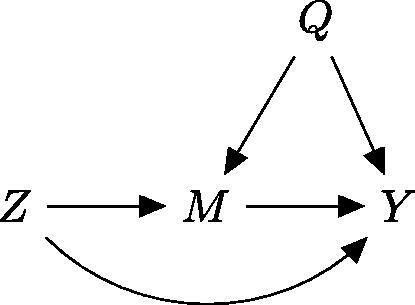
B.1 Mediator ignorability is violated

First, note that $Z\perp \text{}\perp \{Y(b,1),M(w),M(b)\}$, because Z is a function of U_Z , and $\{Y(b,1),M(w),M(b)\}$ are functions of U_Y, U_Q , and U_M , which are jointly independent of U_Z . Now, applying this fact and conditioning on Q, we have that,$$\begin{array}{cc}\mathrm{Pr}\hfill & (Y(b,1)=1|M(w)=m_w,M(b)=1,Z=z)\hfill \\ \hfill & =\mathrm{Pr}(Y(b,1)=1|M(w)=m_w,M(b)=1)\hfill \\ \hfill & =\sum _{q=1}^4\mathrm{Pr}(Y(b,1)=1|M(w)=m_w,M(b)=1,Q=q)\hfill \\ \hfill & ·\mathrm{Pr}(Q=q|M(w)=m_w,M(b)=1)\hfill \\ \hfill & =\sum _{q=1}^4\mathrm{Pr}(f_Y(b,1,q,U_Y)=1|M(w)=m_w,M(b)=1,Q=q)\hfill \\ \hfill & ·\mathrm{Pr}(Q=q|M(w)=m_w,M(b)=1).\hfill \end{array}$$

Next, observe that $f_Y(b,1,q,U_Y)=\mathrm{ }1(q=1)$, and so(B.19) $$\begin{array}{c}\mathrm{Pr}(Y(b,1)=1 | M(w)=m_w,M(b)=1,Z=z)\\ =\mathrm{Pr}(Q=1 | M(w)=m_w,M(b)=1)\\ =\frac{\mathrm{Pr}(M(w)=m_w,M(b)=1 | Q=1)·\mathrm{Pr}(Q=1)}{\sum _{q=1}^4\mathrm{Pr}(M(w)=m_w,M(b)=1 | Q=q)·\mathrm{Pr}(Q=q)}\\ =\frac{\mathrm{Pr}(M(w)=m_w,M(b)=1 | Q=1)}{\sum _{q=1}^4\mathrm{Pr}(M(w)=m_w,M(b)=1 | Q=q)}.\end{array}$$(B.19)

The second equality above follows from Bayes’ rule, and the third follows from the fact that $\mathrm{Pr}(Q=q)=1/4$.

Finally, we compute $\mathrm{Pr}(M(w)=m_w,M(b)=1 | Q=q)$. Note that(B.20) $$\begin{array}{c}M(w)=f_M(w,Q,U_M)\\ =1\left(U_M\le \frac{1(Q=1)+1(Q=2)}{2}\right)\\ =\{\begin{array}{cc}1(U_M\le 1/2)\hfill & Q\in \{1,2\},\hfill \\ 0\hfill & \text{otherwise}.\hfill \end{array}\end{array}$$(B.20)

Likewise,(B.21) $$\begin{array}{c}M(b)=f_M(b,Q,U_M)\\ =1(U_M\le (1(Q=1)+1(Q=3)))\\ =\{\begin{array}{cc}1\hfill & Q\in \{1,3\},\hfill \\ 0\hfill & \text{otherwise}.\hfill \end{array}\end{array}$$(B.21)

As a result,$$\begin{array}{cc}\mathrm{Pr}(M(w)=m_w,M(b)=1 | Q=q)\hfill & =\{\begin{array}{cc}1/2\hfill & q=1,\hfill \\ 1\hfill & q=3\wedge m_w=0,\hfill \\ 0\hfill & \text{otherwise}.\hfill \end{array}\hfill \end{array}$$

Thus, by Equation (B.19)(B.19) $$\begin{array}{c}\mathrm{Pr}(Y(b,1)=1 | M(w)=m_w,M(b)=1,Z=z)\\ =\mathrm{Pr}(Q=1 | M(w)=m_w,M(b)=1)\\ =\frac{\mathrm{Pr}(M(w)=m_w,M(b)=1 | Q=1)·\mathrm{Pr}(Q=1)}{\sum _{q=1}^4\mathrm{Pr}(M(w)=m_w,M(b)=1 | Q=q)·\mathrm{Pr}(Q=q)}\\ =\frac{\mathrm{Pr}(M(w)=m_w,M(b)=1 | Q=1)}{\sum _{q=1}^4\mathrm{Pr}(M(w)=m_w,M(b)=1 | Q=q)}.\end{array}$$(B.19) ,$$\mathrm{Pr}(Y(b,1)=1 | M(w)=1,M(b)=1,Z=z)=1,$$while$$\mathrm{Pr}(Y(b,1)=1 | M(w)=0,M(b)=1,Z=z)=\frac{1}{3}.$$

Therefore, $Y(b,1)\cancel{\perp \text{}\perp }M(w) | M(b)=1,Z=z$, meaning that mediator ignorability does not hold.

B.2 Subset ignorability holds

Similar to the above, we have that(B.22) $$\begin{array}{c}Y(b,1)=f_Y(b,1,Q,U_Y)\\ =1(U_Y\le 1(Q=1))\\ =\{\begin{array}{cc}1\hfill & Q=1,\hfill \\ 0\hfill & \text{otherwise},\hfill \end{array}\end{array}$$(B.22) and(B.23) $$\begin{array}{c}Y(w,1)=f_Y(w,1,Q,U_Y)\\ =1(U_Y\le 1(Q=1)/2)\\ =\{\begin{array}{cc}1(U_Y\le 1/2)\hfill & Q=1,\hfill \\ 0\hfill & \text{otherwise}.\hfill \end{array}\end{array}$$(B.23)

Now, as before, $Z\perp \text{}\perp \{Q,M(w),M(b)\}$, since Z is a function of U_Z , and $\{Q,M(w),M(b)\}$ are functions of U_Q and U_M , which are jointly independent of U_Z . Consequently,(B.24) $$\begin{array}{c}\mathrm{Pr}(Q=1 | M=1,Z=z)=\mathrm{Pr}(Q=1 | M(z)=1,Z=z)\\ =\mathrm{Pr}(Q=1 | M(z)=1)\\ =\frac{\mathrm{Pr}(M(z)=1 | Q=1)·\mathrm{Pr}(Q=1)}{\sum _{q=1}^4\mathrm{Pr}(M(z)=1 | Q=q)·\mathrm{Pr}(Q=q)}\\ =\frac{1}{2},\end{array}$$(B.24) where the last equality follows from Equations (B.20)(B.20) $$\begin{array}{c}M(w)=f_M(w,Q,U_M)\\ =1\left(U_M\le \frac{1(Q=1)+1(Q=2)}{2}\right)\\ =\{\begin{array}{cc}1(U_M\le 1/2)\hfill & Q\in \{1,2\},\hfill \\ 0\hfill & \text{otherwise}.\hfill \end{array}\end{array}$$(B.20) and (B.21), together with the fact that $\mathrm{Pr}(Q=q)=1/4$, and that $U_M\perp \text{}\perp Q$.

Finally, conditioning on Q, we have$$\begin{array}{cc}\hfill & \mathrm{Pr}(Y(b,1)=1 | M=1,Z=z)\hfill \\ \hfill & =\sum _{q=1}^4\mathrm{Pr}(Y(b,1)=1 | M=1,Z=z,Q=q)\hfill \\ \hfill & \hspace{1em}·\mathrm{Pr}(Q=q | M=1,Z=z)\hfill \\ \hfill & =\mathrm{Pr}(Q=1 | M=1,Z=z)\hfill \\ \hfill & =\frac{1}{2},\hfill \end{array}$$where the second equality follows from Equation (B.22)(B.22) $$\begin{array}{c}Y(b,1)=f_Y(b,1,Q,U_Y)\\ =1(U_Y\le 1(Q=1))\\ =\{\begin{array}{cc}1\hfill & Q=1,\hfill \\ 0\hfill & \text{otherwise},\hfill \end{array}\end{array}$$(B.22) , and the third from Equation (B.24)(B.24) $$\begin{array}{c}\mathrm{Pr}(Q=1 | M=1,Z=z)=\mathrm{Pr}(Q=1 | M(z)=1,Z=z)\\ =\mathrm{Pr}(Q=1 | M(z)=1)\\ =\frac{\mathrm{Pr}(M(z)=1 | Q=1)·\mathrm{Pr}(Q=1)}{\sum _{q=1}^4\mathrm{Pr}(M(z)=1 | Q=q)·\mathrm{Pr}(Q=q)}\\ =\frac{1}{2},\end{array}$$(B.24) . Similarly,$$\begin{array}{cc}\hfill & \mathrm{Pr}(Y(w,1)=1 | M=1,Z=z)\hfill \\ \hfill & =\sum _{q=1}^4\mathrm{Pr}(Y(w,1)=1 | M=1,Z=z,Q=q)\hfill \\ \hfill & \hspace{1em}·\mathrm{Pr}(Q=q | M=1,Z=z)\hfill \\ \hfill & =\mathrm{Pr}(U_Y\le 1/2 | M=1,Z=z,Q=1)·\mathrm{Pr}(Q=1 | M=1,Z=z)\hfill \\ \hfill & =\mathrm{Pr}(U_Y\le 1/2)·\mathrm{Pr}(Q=1 | M=1,Z=z)\hfill \\ \hfill & =\frac{1}{4},\hfill \end{array}$$ where the second equality follows from Equation (B.23)(B.23) $$\begin{array}{c}Y(w,1)=f_Y(w,1,Q,U_Y)\\ =1(U_Y\le 1(Q=1)/2)\\ =\{\begin{array}{cc}1(U_Y\le 1/2)\hfill & Q=1,\hfill \\ 0\hfill & \text{otherwise}.\hfill \end{array}\end{array}$$(B.23) , the third from the fact that $U_Y\perp \text{}\perp \{M,Z,Q\}$, and the fourth from Equation (B.24)(B.24) $$\begin{array}{c}\mathrm{Pr}(Q=1 | M=1,Z=z)=\mathrm{Pr}(Q=1 | M(z)=1,Z=z)\\ =\mathrm{Pr}(Q=1 | M(z)=1)\\ =\frac{\mathrm{Pr}(M(z)=1 | Q=1)·\mathrm{Pr}(Q=1)}{\sum _{q=1}^4\mathrm{Pr}(M(z)=1 | Q=q)·\mathrm{Pr}(Q=q)}\\ =\frac{1}{2},\end{array}$$(B.24) . Therefore, $\mathrm{Pr}(Y(b,1)=y | M=1,Z=b)=\mathrm{Pr}(Y(b,1) | M=1,Z=w)$ and similarly for $Y(w,1)$. In particular, this means that $Y(z,1)\perp \text{}\perp Z | M=1$, and so subset ignorability holds. □

Appendix C:

Extending Theorem 1 to Allow for Continuous Covariates

Theorem 1

in the main text shows that subset ignorability—together with overlap—implies the sate${}_M$ is nonparametrically identified, where, for simplicity, we proved the result for discrete covariates X. We now extend that result to allow for continuous covariates. At a conceptual level, the extension is straightforward: we first condition on X, then appeal to subset ignorability to condition on Z, and, finally, use consistency to replace potential outcomes by their observed values. In the general case, however, typically $\mathrm{Pr}(X=x)=0$, and so one must take care to define expressions that nominally condition on these probability-zero events.

Recall that in the discrete case, the primary conditional expectations, treated as functions of z and x, are of the form(C.25) $$\begin{array}{c}\mathbb{E}[Y | Z=z,X=x,M=1]\\ \hspace{1em}=\sum _{y}y\frac{\mathrm{Pr}(Y=y,Z=z,X=x | M=1)}{\mathrm{Pr}(Z=z,X=x | M=1)}\\ \hspace{1em}=\sum _{y}y\frac{\mathrm{Pr}(Y=y,Z=z,X=x | M=1)}{\mathrm{Pr}(Z=z | X=x,M=1)\mathrm{Pr}(X=x | M=1)}.\end{array}$$(C.25)

Overlap ensures that the denominator in (C.25) is nonzero, and, accordingly, that the conditional expectation is well-defined. In the continuous case, to address conditioning on probability-zero events, conditional probabilities are defined as random variables rather than simple numeric quantities (cf. Billingsley 2008). Further, if the random variables $\mathrm{Pr}(Z=z | X,M=1)>0$ a.s. for $z\in \{w,b\}$—a condition that we call generalized overlap—then the expression $\mathbb{E}[Y | Z=z,X=x,M=1]$ is a well-defined function of z and x, as in the discrete case, up to a set of measure zero with respect to the pushforward measure ${\mu }_{X\mathrm{ }|\mathrm{ }M=1}$ for each fixed z.^18,19

We now state and prove the extension of Theorem 1, with the understanding that the conditional probabilities and expectations below are defined according to the usual measure-theoretic conventions.

Theorem C.1.

Suppose $Y(z,1)$, Z, M, and X satisfy subset ignorability, and that generalized overlap holds—that is, for $z\in \{b,w\},\mathrm{Pr}(Z=z | X,M=1)>0$ a.s. Then, the sate${}_M$ equals(C.26) $$\begin{array}{cc}\hfill & {\int }_{\mathcal{X}}\mathbb{E}[Y | Z=b,X=x,M=1] \mathrm{d}{F}_{X\mathrm{ }|\mathrm{ }M=1}\hfill \\ \hfill & \hspace{1em}-{\int }_{\mathcal{X}}\mathbb{E}[Y | Z=w,X=x,M=1] \mathrm{d}{F}_{X\mathrm{ }|\mathrm{ }M=1},\hfill \end{array}$$(C.26) where $\mathcal{X}$ denotes the range of X and $\mathrm{d}{F}_{X\mathrm{ }|\mathrm{ }M=1}$ denotes integration over $\mathcal{X}$ with respect to the pushforward measure ${\mu }_{X\mathrm{ }|\mathrm{ }M=1}$.

Proof.

By conditioning on X, we have,(C.27) $$\begin{array}{c}{\text{SATE}}_M=\mathbb{E}[Y(b,1)-Y(w,1) | M=1]\\ ={\int }_{\mathcal{X}}\mathbb{E}[Y(b,1)-Y(w,1) | X=x,M=1] \mathrm{d}{F}_{X\mathrm{ }|\mathrm{ }M=1}\\ ={\int }_{\mathcal{X}}\mathbb{E}[Y(b,1) | X=x,M=1]\\ \hspace{1em}-\mathbb{E}[Y(w,1) | X=x,M=1] \mathrm{d}{F}_{X\mathrm{ }|\mathrm{ }M=1}.\end{array}$$(C.27)

Now, subset ignorability gives that, a.s.,(C.28) $$\mathbb{E}[Y(z,1)|X=x,M=1]=\mathbb{E}[Y(z,1)|X=x,Z=z,M=1],$$(C.28) where generalized overlap ensures that the right-hand side of Equation (C.28)(C.28) $$\mathbb{E}[Y(z,1)|X=x,M=1]=\mathbb{E}[Y(z,1)|X=x,Z=z,M=1],$$(C.28) is well-defined up to a set of measure zero with respect to $\mathrm{d}{F}_{X\mathrm{ }|\mathrm{ }M=1}$. Substituting this expression into Equation (C.27)(C.27) $$\begin{array}{c}{\text{SATE}}_M=\mathbb{E}[Y(b,1)-Y(w,1) | M=1]\\ ={\int }_{\mathcal{X}}\mathbb{E}[Y(b,1)-Y(w,1) | X=x,M=1] \mathrm{d}{F}_{X\mathrm{ }|\mathrm{ }M=1}\\ ={\int }_{\mathcal{X}}\mathbb{E}[Y(b,1) | X=x,M=1]\\ \hspace{1em}-\mathbb{E}[Y(w,1) | X=x,M=1] \mathrm{d}{F}_{X\mathrm{ }|\mathrm{ }M=1}.\end{array}$$(C.27) , and then appealing to consistency to replace potential outcomes with their observed values, we have$$\begin{array}{cc}{\text{SATE}}_M\hfill & ={\int }_{\mathcal{X}}\mathbb{E}[Y(b,1) | X=x,Z=b,M=1]\hfill \\ \hfill & \hspace{1em}-\mathbb{E}[Y(w,1) | X=x,Z=w,M=1] \mathrm{d}{F}_{X\mathrm{ }|\mathrm{ }M=1}\hfill \\ \hfill & ={\int }_{\mathcal{X}}\mathbb{E}[Y(Z,M) | X=x,Z=b,M=1]\hfill \\ \hfill & \hspace{1em}-\mathbb{E}[Y(Z,M) | X=x,Z=w,M=1] \mathrm{d}{F}_{X\mathrm{ }|\mathrm{ }M=1}\hfill \\ \hfill & ={\int }_{\mathcal{X}}\mathbb{E}[Y | X=x,Z=b,M=1]\hfill \\ \hfill & \hspace{1em}-\mathbb{E}[Y | X=x,Z=w,M=1] \mathrm{d}{F}_{X\mathrm{ }|\mathrm{ }M=1}.\hfill \end{array}$$

Fig. D.2. Breakdown of age by gender of individuals arrested for a felony offense between 2013 and 2019 in a major U.S. county, as analyzed in Section 4.

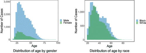
All of the quantities in Equation (C.26)(C.26) $$\begin{array}{cc}\hfill & {\int }_{\mathcal{X}}\mathbb{E}[Y | Z=b,X=x,M=1] \mathrm{d}{F}_{X\mathrm{ }|\mathrm{ }M=1}\hfill \\ \hfill & \hspace{1em}-{\int }_{\mathcal{X}}\mathbb{E}[Y | Z=w,X=x,M=1] \mathrm{d}{F}_{X\mathrm{ }|\mathrm{ }M=1},\hfill \end{array}$$(C.26) (i.e., the distribution of X and the conditional expectations) are functions of observables, establishing that the sate ${}_M$ is identified by data on second-stage decisions. One may adopt a variety of approaches to estimate the terms in Equation (C.26)(C.26) $$\begin{array}{cc}\hfill & {\int }_{\mathcal{X}}\mathbb{E}[Y | Z=b,X=x,M=1] \mathrm{d}{F}_{X\mathrm{ }|\mathrm{ }M=1}\hfill \\ \hfill & \hspace{1em}-{\int }_{\mathcal{X}}\mathbb{E}[Y | Z=w,X=x,M=1] \mathrm{d}{F}_{X\mathrm{ }|\mathrm{ }M=1},\hfill \end{array}$$(C.26) , including model-based strategies, as we do in Section 4. One may also adopt nonparametric estimation strategies, wherein continuous covariates are appropriately binned into discrete sets. For further treatment of these issues, see, for example, Gelman et al. (2013), Friedman, Hastie, and Tibshirani (2001), and Tsybakov (2008).

Appendix D:

Summary Statistics of Prosecution Dataset

We present summary statistics, disaggregated by demographic group, of the dataset used to conduct the empirical analysis of prosecutorial charging decisions in Section 4.

References

- Ayres, I. (2002), “Outcome Tests of Racial Disparities in Police Practices,” Justice Research and Policy, 4, 131–142. DOI: 10.3818/JRP.4.1.2002.131.
- Balsa, A. I., McGuire, T. G., and Meredith, L. S. (2005), “Testing for Statistical Discrimination in Health Care,” Health Services Research, 40, 227–252. DOI: 10.1111/j.1475-6773.2005.00351.x.
- Baum, S., and Goodstein, E. (2005), “Gender Imbalance in College Applications: Does it Lead to a Preference for Men in the Admissions Process?” Economics of Education Review, 24, 665–675.
- Berg, N., and Lien, D. (2002), “Measuring the Effect of Sexual Orientation on Income: Evidence of Discrimination?” Contemporary Economic Policy, 20, 394–414.
- Bertrand, M., and Mullainathan, S. (2004), “Are Emily and Greg More Employable than Lakisha and Jamal? A Field Experiment on Labor Market Discrimination,” American Economic Review, 94, 991–1013.
- Billingsley, P. (2008), Probability and Measure, New Delhi: Wiley.
- Carnegie, N. B., Harada, M., and Hill, J. L. (2016), “Assessing Sensitivity to Unmeasured Confounding Using a Simulated Potential Confounder,” Journal of Research on Educational Effectiveness, 9, 395–420.
- Chohlas-Wood, A., Nudell, J., Yao, K., Lin, Z., Nyarko, J., and Goel, S. (2021), “Blind Justice: Algorithmically Masking Race in Charging Decisions,” in Proceedings of the 2021 AAAI/ACM Conference on AI, Ethics, and Society, pp. 35–45.
- Cinelli, C., and Hazlett, C. (2020), “Making Sense of Sensitivity: Extending Omitted Variable Bias,” Journal of the Royal Statistical Society, Series B, 82, 39–67.
- Cornfield, J., Haenszel, W., Hammond, E. C., Lilienfeld, A. M., Shimkin, M. B., and Wynder, E. L. (1959), “Smoking and Lung Cancer: Recent Evidence and a Discussion of Some Questions,” Journal of the National Cancer Institute, 22, 173–203.
- Dorie, V., Harada, M., Carnegie, N. B., and Hill, J. (2016), “A Flexible, Interpretable Framework for Assessing Sensitivity to Unmeasured Confounding,” Statistics in Medicine, 35, 3453–3470.
- Edelman, B. G., and Luca, M. (2014), “Digital Discrimination: The Case of airbnb.com,” Harvard Business School NOM Unit Working Paper, 14–054.
- Franks, A., D’Amour, A., and Feller, A. (2019), “Flexible Sensitivity Analysis for Observational Studies Without Observable Implications,” Journal of the American Statistical Association, 115, 1730–1746.
- Friedman, J., Hastie, T., and Tibshirani, R. (2001), The Elements of Statistical Learning. Springer Series in Statistics, New York: Springer.
- Fryer Jr, R. G. (2019), “An Empirical Analysis of Racial Differences in Police use of Force,” Journal of Political Economy, 127, 1210–1261.
- Gelman, A., Fagan, J., and Kiss, A. (2007), “An Analysis of the New York City Police Department’s “Stop-and-Frisk” Policy in the Context of Claims of Racial Bias,” Journal of the American Statistical Association, 102, 813–823.
- Gelman, A., Carlin, J. B., Stern, H. S., Dunson, D. B., Vehtari, A., and Rubin, D. B. (2013), Bayesian Data Analysis, Boca Raton, FL: CRC Press.
- Goel, S., Perelman, M., Shroff, R., and Sklansky, D. A. (2017), “Combatting Police Discrimination in the Age of Big Data,” New Criminal Law Review: An International and Interdisciplinary Journal, 20, 181–232.
- Goldin, C., and Rouse, C. (2000), “Orchestrating Impartiality: The Impact of “Blind” Auditions on Female Musicians,” American Economic Review, 90, 715–741.
- Greenberg, D., Gershenson, C., and Desmond, M. (2016), “Discrimination in Evictions: Empirical Evidence and Legal Challenges,” Harvard Civil Rights-Civil Liberties Law Review, 51, 115–158.
- Greiner, D. J., and Rubin, D. B. (2011), “Causal Effects of Perceived Immutable Characteristics,” Review of Economics and Statistics, 93, 775–785.
- Grogger, J., and Ridgeway, G. (2006), “Testing for Racial Profiling in Traffic Stops from Behind a Veil of Darkness,” Journal of the American Statistical Association, 101, 878–887.
- Heckman, J. J. (1979), “Sample Selection Bias as a Specification Error,” Econometrica: Journal of the Econometric Society, 47, 153–161.
- Heckman, J. J., and Durlauf, S. N. (2020), Comment on “An Empirical Analysis of Racial Differences in Police use of Force” by Roland G. Fryer Jr., Journal of Political Economy.
- Hill, J. L. (2011), “Bayesian Nonparametric Modeling for Causal Inference,” Journal of Computational and Graphical Statistics, 20, 217–240.
- Holland, P. W. (1986), “Statistics and Causal Inference,” Journal of the American Statistical Association, 81, 945–960.
- Imai, K., Keele, L., and Tingley, D. (2010a), “A General Approach to Causal Mediation Analysis,” Psychological Methods, 15, 309–334.
- Imai, K., Keele, L., and Yamamoto, T. (2010b), “Identification, Inference and Sensitivity Analysis for Causal Mediation Effects,” Statistical Science, 25, 51–71.
- Imbens, G. W. (2003), “Sensitivity to Exogeneity Assumptions in Program Evaluation,” The American Economic Review, 93, 126–132.
- Imbens, G. W., and Rubin, D. B. (2015), Causal Inference in Statistics, Social, and Biomedical Sciences, New York: Cambridge University Press.
- Jung, J., Corbett-Davies, S., Shroff, R., and Goel, S. (2018), “Omitted and Included Variable Bias in Tests for Disparate Impact,” arXiv preprint arXiv:1809.05651.
- Jung, J., Shroff, R., Feller, A., and Goel, S. (2020), “Bayesian Sensitivity Analysis for Offline Policy Evaluation,” in Proceedings of the AAAI/ACM Conference on AI, Ethics, and Society, pp. 64–70.
- Knox, D., Lowe, W., and Mummolo, J. (2020), “Administrative Records Mask Racially Biased Policing,” American Political Science Review, 114, 619–637.
- MacDonald, J., and Raphael, S. (2021), “Effect of Scaling Back Punishment on Racial and Ethnic Disparities in Criminal Case Outcomes,” Criminology & Public Policy, 19, 1139–1164.
- McCandless, L. C., and Gustafson, P. (2017), “A Comparison of Bayesian and Monte Carlo Sensitivity Analysis for Unmeasured Confounding,” Statistics in Medicine, 36, 2887–2901.
- McCandless, L. C., Gustafson, P., and Levy, A. (2007), “Bayesian Sensitivity Analysis for Unmeasured Confounding in Observational Studies,” Statistics in Medicine, 26, 2331–2347.
- Munnell, A. H., Tootell, G. M. B., Browne, L. E., and McEneaney, J. (1996), “Mortgage Lending in Boston: Interpreting HMDA Data,” The American Economic Review, 86, 25–53.
- Pearl, J. (2009), Causality, Cambridge: Cambridge University Press.
- Pearl, J. (2015), “Conditioning on Post-Treatment Variables,” Journal of Causal Inference, 3, 131–137.
- Pearl, J., Glymour, M., and Jewell, N. P. (2016), Causal Inference in Statistics: A Primer, Chichester: Wiley.
- Pierson, E., Simoiu, C., Overgoor, J., Corbett-Davies, S., Jenson, D., Shoemaker, A., Ramachandran, V., Barghouty, P., Shroff, R., Phillips, C., and Goel, S. (2020), “A Large-Scale Analysis of Racial Disparities in Police Stops Across the United States,” Nature Human Behaviour, 4, 736–745.
- Rehavi, M. M., and Starr, S. B. (2014), “Racial Disparity in Federal Criminal Sentences,” Journal of Political Economy, 122, 1320–1354.
- Richardson, T., and Robins, J. (2013), “Single World Intervention Graphs (SWIGs): A Unification of the Counterfactual and Graphical Approaches to Causality,” Technical report, Technical Report 128, Center for Statistics and the Social Sciences, Univ. Washington, Seattle, WA.
- Robertson, C., Baughman, S. B., and Wright, M. S. (2019), “Race and Class: A Randomized Experiment with Prosecutors,” Journal of Empirical Legal Studies, 16, 807–847.
- Robins, J. (1986), “A New Approach to Causal Inference in Mortality Studies with a Sustained Exposure Period—Application to Control of the Healthy Worker Survivor Effect,” Mathematical Modelling, 7, 1393–1512.
- Robins, J. M., Richardson, T. S., and Shpitser, I. (2020), “An Interventionist Approach to Mediation Analysis.”
- Rosenbaum, P. R., and Rubin, D. B. (1983a). “The Central Role of the Propensity Score in Observational Studies for Causal Effects,” Biometrika, 70, 41–55.
- Rosenbaum, P. R., and Rubin, D. B. (1983b), “Assessing Sensitivity to an Unobserved Binary Covariate in an Observational Study with Binary Outcome,” Journal of the Royal Statistical Society, 45, 212–218.
- Sekhon, J. (2008), “The Neyman–Rubin Model of Causal Inference and Estimation via Matching Methods,” in The Oxford Handbook of Political Methodology, eds. J. Box-Steffensmeier, H. Brady, and D. Collier, Oxford: Oxford University Press.
- Spencer, K. B., Charbonneau, A. K., and Glaser, J. (2016), “Implicit Bias and Policing,” Social and Personality Psychology Compass, 10, 50–63.
- Tsybakov, A. B. (2008), Introduction to Nonparametric Estimation, New York: Springer.
- Word, D., and Perkins, C. (1996), Building a Spanish Surname List for the 1990’s: A New Approach to an Old Problem, Washington, DC: Population Division, US Bureau of the Census.
- Word, D., Coleman, C., Nunziata, R., and Kominski, R. (2008), “Demographic Aspects of Surnames from Census 2000,” Technical report, U.S. Census Bureau Population Division. Available at http://www2.census.gov/topics/genealogy/2000surnames/surnames.pdf.
- Zhao, Q., Keele, L. J., Small, D. S., and Joffe, M. M. (2021), “A Note on Post-treatment Selection in Studying Racial Discrimination in Policing,” American Political Science Review, 1–14.