Block-pulse functions approach to numerical solution of Abel’s integral equation

Abstract

This study aims to present a computational method for solving Abel’s integral equation of the second kind. The introduced method is based on the use of Block-pulse functions (BPFs) via collocation method. Abel’s integral equations as singular Volterra integral equations are hard and heavy in computation, but because of the properties of BPFs, as is reported in examples, this method is more efficient and more accurate than some other methods for solving this class of integral equations. On the other hand, the benefit of this method is low cost of computing operations. The applied method transforms the singular integral equation into triangular linear algebraic system that can be solved easily. An error analysis is worked out and applications are demonstrated through illustrative examples.

Keywords:

• Abel’s integral equation
• Block-pulse functions
• collocation method

Public Interest Statement

Abel’s equation is one of the integral equations derived directly from a concrete problem of mechanics or physics (without passing through a differential equation). Historically, Abel’s problem is the first one that led to the study of integral equations. The construction of high-order methods for the equations is, however, not an easy task because of the singularity in the weakly singular kernel. Our method applied block-pulse functions via collocation method for solving the mentioned problem and converts it into a triangular algebraic system. Compared with some other presented methods, this method significantly reduces the computational complexity and is more accurate.

1. Introduction

The past two decades have been witnessing a strong interest among physicists, engineers, and mathematicians for the theory and numerical modeling of integral and integro-differential equations. These equations are solved analytically; see, for example, the excellent book by Mushkelishvili (1953), and the references therein. The generalized Abel’s integral equation on a finite segment appeared for the first time in the paper of Zeilon (1922). A comprehensive reference on Abel-type equations, including an extensive list of applications, can be found in Gorenflo and Vessella (1991) and Wazwaz (1997). The construction of high-order methods for the equations is, however, not an easy task because of the singularity in the weakly singular kernel. In fact, in this case the solution $y$ is generally not differentiable at the endpoints of the interval, see Schneider (1981) and Vainikko and Pedas (1981), and due to this, to the best of the authors? knowledge the best convergence rate ever achieved remains only at polynomial order. For example, if we set uniform meshes with $n+1$ grid points and apply the spline method so for order $m$, then the convergence rate is only $O(n^{-2p})$ at most (Schneider, 1979; Graham, 1982), and it cannot be improved by increasing $m$. One way of remedying this is to introduce graded meshes. Then the rate is improved to $O(n^{-m})$ (Vainikko & Uba, 1981) which now depends on $m$, but still at polynomial order. Fettis (1964) proposed a numerical form of the solution to Abel equation by using the Gauss–Jacobi quadrature rule. Piessens and Verbaeten (1973) and Piessens (2000) developed an approximate solution to Abel equation by means of the Chebyshev polynomials of the first kind. Numerical solutions of weakly singular Volterra integral equations were introduced by many researchers, such as Baratella and Orsi (2004) and Abdou and Nasr (2003). Yanzhao, Min, Liping, and Yuesheng (2007) applied hybrid collocation method for solving these equations. Ishik, Sezer, and Gney (2011) used Bernstein series solution for solving linear integro-differential equations with weakly singular kernels. Wazwaz (2002) studied on singular initial value problems in the second-order ordinary differential equations. Yousefi (2006) applied Legendre wavelets to transform Abel integral equation to a algebraic system.

The aim of this work is to present a computational method for solving special case of singular Volterra integral equations of the second kind as named Abel’s integral equation defined as(1) $$\begin{array}{c}\hfill y(x)=f(x)-{\int }_0^x\frac{y(t)}{\sqrt{x-t}}dt\end{array}$$(1)

where $f\in L^2([0,T])$. Our method consists of reducing the given weakly singular integral equation to a set of algebraic equations by expanding the unknown function using block-pulse functions (BPFs) with unknown coefficients. Collocation method is utilized to evaluate the unknown coefficients. Because of orthogonality, disjointness and having completeness properties of these functions, the operational matrix of method is a sparse lower triangular matrix. Without loss of generality, we may consider $[0,T]=[0,1]$.

The paper is organized as follows: In the next section, we discuss BPFs, their key properties and function approximation by them. In Section 3, we give the description and development of the method for solving singular integral equation. Error analysis and convergence of the method is discussed in Section 4. In Section 5 for showing the efficiency of this method, some numerical examples are presented. Section 6 is devoted to the conclusion of this paper.

2. Block-pulse functions

BPFs are studied by many authors and applied for solving different problems, for example see Steffens (2006).

A $k$-set of BPFs over the interval $[0,T)$ is defined as(2) $$\begin{array}{c}\hfill B_i(t)=\left\{\begin{array}{cc}1,\hfill & \frac{iT}{k}\le t<\frac{(i+1)T}{k}\hfill \\ 0,\hfill & \text{elsewhere}\hfill \end{array}\right.\end{array}$$(2) $$i=0,1,\dots ,k-1,$$

with a positive integer value for $k$. In this paper, it is assumed that $T=1$, so BPFs are defined over $[0,1)$. BPFs have some main properties, the most important of these properties are disjointness, orthogonality, and completeness.

(I)	The disjointness property can be clearly obtained from the definition of BPFs(3) $$\begin{array}{c}\hfill B_i(t)B_j(t)=\left\{\begin{array}{cc}{B}_i(t),\hfill & i=j\hfill \\ 0,\hfill & i\ne j\hfill \end{array}\right.i,j=0,1,\dots ,k-1\end{array}$$(3)
(II)	The orthogonality property of these functions is(4) $$\begin{array}{c}\hfill ⟨B_i(t),B_j(t)⟩={\int }_0^1{B}_i(t)B_j(t)dt=\left\{\begin{array}{cc}\frac{1}{k},\hfill & i=j\hfill \\ 0,\hfill & i\ne j\hfill \end{array}\right.i,j=0,1,\dots ,k-1\end{array}$$(4)
(III)	The third property is completeness. For every $y\in L^2[0,1)$, when $k$ approaches to the infinity, Parseval’s identity holds, that is$$\begin{array}{c}\hfill {\int }_0^1{y}^2(t)dt=\sum _{i=1}^{\infty }{c}_i^2{\Vert B_i(t)\Vert }^2\end{array}$$ where(5) $$\begin{array}{c}\hfill c_i=k{\int }_0^{1}f(t)B_i(t)dt\end{array}$$(5)

A function $y(t)$ defined over the interval $[0,1)$ may be expanded by a $k-$set of BPFs as(6) $$\begin{array}{c}\hfill y(t)\simeq y_k(t)=\sum _{i=0}^{k-1}{c}_i{B}_i(t)={\mathbf{C}}^T\mathbf{B}(t)\end{array}$$(6)

where $c_i=k⟨y(t),B_i(t)⟩,$ and$$\begin{array}{c}\hfill \mathbf{C}={\left(c_0,c_1,\dots ,c_{k-1}\right)}^T\end{array}$$

and$$\begin{array}{c}\hfill \mathbf{B}(t)={\left(B_0(t),B_1(t),\dots ,B_{k-1}(t)\right)}^T\end{array}$$

where $c_i$ are samples of $y$, for example $c_i=y(\frac{i}{k})$ for $i=0,1,\dots ,k-1$, and as a result there is no need for integration. The vector $C$ is called the 1D-BPFs coefficient vector.

3. Numerical implementation

Consider the Abel’s integral equation$$\begin{array}{c}\hfill y(x)=f(x)-{\int }_0^x\frac{y(t)}{\sqrt{x-t}}dt,x\in [0,1]\end{array}$$

where $f\in L^2(\mathbb{R})$ is known and $y(t)$ is the unknown function to be determined. Now by substituting Equation 6 into Equation 1, we obtain(7) $$\begin{array}{cc}\hfill {\mathbf{C}}^T\mathbf{B}(x)& =f(x)-{\int }_0^x\frac{{\mathbf{C}}^T\mathbf{B}(t)}{\sqrt{x-t}}dt\hfill \\ \hfill & =f(x)-{\mathbf{C}}^T{\int }_0^x\frac{\mathbf{B}(t)}{\sqrt{x-t}}dt\hfill \end{array}$$(7)

by evaluating Equation 7 at the collocation points $x_j=\frac{j-1/2}{k},j=1,2,\cdots ,k,$ we obtain(8) $$\begin{array}{c}\hfill {\mathbf{C}}^T\mathbf{B}(x_j)=f(x_j)-{\mathbf{C}}^T{\int }_0^{x_j}\frac{\mathbf{B}(t)}{\sqrt{x_j-t}}dt\end{array}$$(8)

by considering $\mathbf{B}(x_j)={\mathbf{e}}_j$ (the $j$-th column of identity matrix), we can rewrite Equation 8 as follows(9) $$\begin{array}{c}\hfill c_j=f(x_j)-{\mathbf{C}}^T{\int }_0^{x_j}\frac{\mathbf{B}(t)}{\sqrt{x_j-t}}dt\end{array}$$(9)

Now for computing the unknown coefficients $c_j$, we introduce a recursive formula.

Figure 1. Exact and approximation solution of Example 1 in $k=32$.

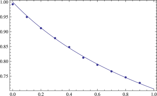
Figure 2. Exact and approximation solution of Example 1 in $k=64$.

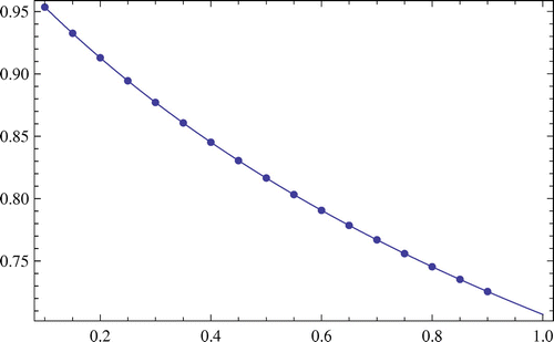
Figure 3. Exact and approximation solution of Example 2 in $k=32$.

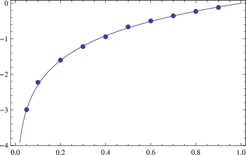
Figure 4. Exact and approximation solution of Example 2 in $k=64$.

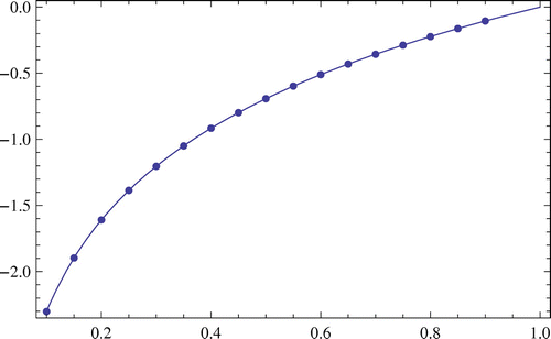
Table 1. Exact and approximate solutions of Example 1

	Approximate			L. W [19]
$x$	$k=16$	$k=32$	$k=64$	$k=1,M=5$	Exact
$0$	0.99734	0.999123	0.999993	0.999432	1
$0.2$	0.911748	0.912305	0.912873	0.91232	0.912871
$0.4$	0.848041	0.845156	0.845154	0.8453212	0.845154
$0.6$	0.788293	0.790527	0.790562	0.7905387	0.790569
$0.8$	0.746027	0.745361	0.745316	0.745342	0.745356
$1$	0.70423	0.70712	0.707103	0.707163	0.707107

Table 2. Exact and approximate solutions of Example 2

	Approximate			L. W [19]
$x$	$k=16$	$k=32$	$k=64$	$k=1,M=5$	Exact
0.2	-1.609841	-1.60942	-1.60944	-1.60927	-1.60944
0.4	-0.916390	-0.916211	-0.916291	-0.916238	-0.916291
0.6	-0.51054	-0.510832	-0.510826	-0.51046	-0.510826
0.8	-0.223750	-0.223101	-0.223144	-0.223575	-0.223144
1	0.00042	0.000001	0	0.00013	0

The unknown coefficient $c_j$ satisfies the following recursive relation:(10) $$\begin{array}{c}\hfill c_j=f(x_j)-\sum _{i=1}^{j-1}{c}_i{\int }_{\frac{i-1}{k}}^{\frac{i}{k}}\frac{1}{\sqrt{x_j-t}}dt-c_j{\int }_{\frac{j-1}{k}}^{\frac{j-1/2}{k}}\frac{1}{\sqrt{x_j-t}}dt\end{array}$$(10)

where$$\begin{array}{c}\hfill c_1=f(x_1)-c_1{\int }_0^{\frac{1}{2k}}\frac{1}{\sqrt{x_1-t}}dt\end{array}$$

The linear system of Equation 10 is a lower triangular system which can be solved easily by forward substitution with $O(k^2)$ operations. If we calculate a table of values of $c_j,j=1,2,\dots ,k$, then the coefficients $c_j$ for every large $k$, can be calculated . The cost of calculating such table is relatively cheap. To prove this, fist note that$$\begin{array}{cc}\hfill {\int }_0^{x_j}\frac{\mathbf{B}(t)}{\sqrt{x_j-t}}dt& ={\int }_0^{\frac{j-1/2}{k}}\frac{{\left(B_1(t),B_2(t),\dots ,B_k(t)\right)}^T}{\sqrt{x_j-t}}dt\hfill \\ \hfill & =\left({\int }_0^{\frac{1}{k}}\frac{1}{\sqrt{x_j-t}}dt\right).{\left(1,0,0,\dots ,0\right)}^T\hfill \\ \hfill & +\left({\int }_{\frac{1}{k}}^{\frac{2}{k}}\frac{1}{\sqrt{x_j-t}}dt\right).{\left(0,1,0,\dots ,0\right)}^T\hfill \\ \hfill & ⋮\hfill \\ \hfill & +\left({\int }_{\frac{j-2}{k}}^{\frac{j-1}{k}}\frac{1}{\sqrt{x_j-t}}dt\right).{\left(0,\dots ,0,1,0\right)}^T+\left({\int }_{\frac{j-1}{k}}^{\frac{j-1/2}{k}}\frac{1}{\sqrt{x_j-t}}dt\right).{\left(0,\dots ,0,1\right)}^T\hfill \end{array}$$

and in abstract form(11) $$\begin{array}{cc}\hfill {\int }_0^{x_j}\frac{\mathbf{B}(t)}{\sqrt{x_j-t}}& dt=\hfill \\ \hfill & {\left({\int }_0^{\frac{1}{k}}\frac{1}{\sqrt{x_j-t}}dt,\dots ,{\int }_{\frac{j-2}{k}}^{\frac{j-1}{k}}\frac{1}{\sqrt{x_j-t}}dt,{\int }_{\frac{j-1}{k}}^{\frac{j-1/2}{k}}\frac{1}{\sqrt{x_j-t}}dt\right)}^T\hfill \end{array}$$(11)

Substituting Equation 11 in Equation 9 leads to Equation 10 and the proof is complete. $\square$

4. Error analysis

In this section, we give an upper bound for the error of BPFs expansion. Assume that $y^{\prime }(t)\in C[0,1]$, thus$$\exists M>0;\forall t\in (0,1),|y^{\prime }(t)|\le M$$

and suppose $e_i(t)$ be the representation error of BPFs expansion in the subinterval $\left[\frac{i-1}{k},\frac{i}{k}\right)$, that is,$$\begin{array}{cc}\hfill e_i(t)& =c_i{B}_i(t)-y(t)\hfill \\ \hfill & =c_i-y(t)\hfill \end{array}$$

Using mean value theorem, we may proceed as follows(12) $$\begin{array}{cc}\hfill \Vert e_i{\Vert }^2& ={\int }_{\frac{i-1}{k}}^{\frac{i}{k}}{e}_i^2(t)dt\hfill \\ \hfill & ={\int }_{\frac{i-1}{k}}^{\frac{i}{k}}{(c_i-y(t))}^{2}dt\hfill \\ \hfill & ={\left(\frac{i}{k}-(\frac{i-1}{k}))(c_i-y({\mathit{\xi }}_1)\right)}^2\hfill \\ \hfill & =\frac{1}{k}{(c_i-y({\mathit{\xi }}_1))}^2,{\mathit{\xi }}_1\in \left(\frac{i-1}{k},\frac{i}{k}\right)\hfill \end{array}$$(12)

For the coefficient $c_i$, we get(13) $$\begin{array}{cc}\hfill c_i& =k<y(t),B_i(t)>\hfill \\ \hfill & =k{\int }_{\frac{i-1}{k}}^{\frac{i}{k}}y(t)dt\hfill \\ \hfill & =k\left(\frac{i}{k}-\left(\frac{i-1}{k}\right)\right)y({\mathit{\xi }}_2)\hfill \\ \hfill & =y({\mathit{\xi }}_2),{\mathit{\xi }}_2\in \left(\frac{i-1}{k},\frac{i}{k}\right)\hfill \end{array}$$(13)

Substituting Equation 13 into Equation 12 and again using mean value theorem, we obtain(14) $$\begin{array}{cc}\hfill \Vert e_i{\Vert }^2& =\frac{1}{k}{\left(b_i-y({\mathit{\xi }}_1)\right)}^2\hfill \\ \hfill & =\frac{1}{k}{\left(y({\mathit{\xi }}_2)-y({\mathit{\xi }}_1)\right)}^2\hfill \\ \hfill & =\frac{1}{k}{\left({\mathit{\xi }}_2-{\mathit{\xi }}_1\right)}^2{y}^{{}^{\prime }2}(\mathit{\xi })\left({\mathit{\xi }}_1<\mathit{\xi }<{\mathit{\xi }}_2\right)\hfill \\ \hfill & \le \frac{1}{k^3}{M}^2\hfill \end{array}$$(14)

Now, for $i<j$, we have$$\left[\frac{i-1}{k},\frac{i}{k}\right)\cap \left[\frac{j-1}{k},\frac{j}{k}\right)=\mathrm{\varnothing },\Rightarrow {\int }_0^1{e}_i(t)e_j(t)dt=0$$

Putting $e(t)=y_k(t)-y(t)$, we have$$\begin{array}{cc}\hfill {\Vert e\Vert }^2& ={\int }_0^1{e}^2(t)dt\hfill \\ \hfill & ={\int }_0^1{\left(\sum _{i=1}^k{e}_i(t)\right)}^{2}dt\hfill \\ \hfill & ={\int }_0^1\sum _{i=1}^k{e}_i^2(t)dt+2\sum _{i<j}{\int }_0^1{e}_i(t)e_j(t)dt\hfill \\ \hfill & =\sum _{i=1}^k{\int }_0^1{e}_i^2(t)dt\hfill \\ \hfill & =\sum _{i=1}^k{\Vert e_i\Vert }^2\hfill \\ \hfill & \le \frac{1}{k^2}{M}^2\hfill \end{array}$$

hence, $\Vert e(t)\Vert =O(\frac{1}{k}).$

Remark

It is clear that the approximation will be more accurate if $k$ (the number of BPFs) is increased, thus for acheiving better results, using larger $k$ is recommended.

5. Numerical examples

In this section, for showing the accuracy and efficiency of the described method we present some examples. The results for introduced method in this work in different scales of $k$ are presented and compared with the results of some other methods.

Example 1

Consider the equation$$y(x)=\frac{1}{\sqrt{x+1}}+\frac{\mathit{\pi }}{8}-\frac{1}{4}arcsin\left(\frac{1-x}{1+x}\right)-\frac{1}{4}{\int }_0^x\frac{y(t)}{\sqrt{x-t}}dt$$

with the exact solution $y(x)=\frac{1}{\sqrt{x+1}}$. The solution for $y(x)$ is obtained by the method in Section 3 at the scales $k=16,32$, and 64. In Table 1, the exact and approximate solutions of Example 1 both by our method and by Legendre wavelets method (Yousefi, 2006) in some arbitrary points are reported. Comparison with Legendre wavelets expansion, the method of this paper has more accuracy. As proved in Section 4, the error at the level $k=64$ is smaller than the error at the levels $k=16$ and $k=32$.

L.W: Results by Legendre wavelets expansion.

In Figures 1 and 2, pointwise plots are the approximated solution of Example 1 (for $k=32$ and $k=64$, respectively) in some arbitrary points and the others are the plot of exact solution.

Example 2

Consider the equation$$y(x)=-4\sqrt{x}+4\sqrt{x}ln(2)-2\sqrt{x}ln\left(\frac{1}{x}\right)+ln(x)-{\int }_0^x\frac{y(t)}{\sqrt{x-t}}dt$$

with the exact solution $y(x)=ln(x)$. The solution for $y(x)$ is obtained by the method in Section 3 at the scales $k=16,32$, and $64$. In Table 2, we present the exact and approximate solutions of Example 2 both by our method and by Legendre wavelets method (Yousefi, 2006) in some arbitrary points. Comparison with Legendre wavelets expansion, the method of this paper has more accuracy. As proved in Section 4, the error at the level $k=64$ is smaller than the error at the levels $k=16$ and $k=32$.

In Figures 3 and 4, pointwise plots are the approximated solution of Example 2 (for $k=32$ and $k=64$, respectively) in some arbitrary points and the others are the plot of exact solution. Obviously, there is less error between two plot for $k=64$ rather than $k=32$.

6. Conclusions

In the present paper, BPFs with the collocation method are applied to solve the Abel’s integral equation. As for Legendre polynomials, Chebyshev polynomials and other generalized orthogonal polynomials, the calculation procedures are usually too tedious, although some recursive formula are available. The benefits of this method are low cost of setting up the equations and more accuracy and more efficiency of the solution than exiting methods for solving this class of equations. Also, the linear system of Equation 11 is a lower triangular system which can be easily solved by forward substitution with $O(k^2)$ operations, therefore, the count of operations is very low. The approach can be extended to nonlinear Abel integral equation and integro differential equation with little additional work. Further research along these lines is under progress and will be reported in due time.

Acknowledgements

The authors would like to thank University of Bonab for providing facilities and encouraging this work and also thank the anonymous reviewers of this paper for their careful reading, constructive comments, and nice suggestions which have improved the paper very much.

Additional information

Notes on contributors

Monireh Nosrati Sahlan

Monireh Nosrati Sahlan is currently an Associate Professor at the Department of Mathematics and Computer Science, Technical Faculty, University of Bonab, Bonab, Iran. Dr Nosrati Sahlan completed her PhD in 2013 from Iran University of Science and Technology, Tehran, Iran. She completed her MSc in Applied Mathematics at Iran University of Science and Technology, in 2007 and BSc in Mathematics at University of Shahid Madani Azerbaijan. Dr Nosrati Sahlan has about ten years of research experience in various field of Applied Mathematics such as; integral equations, integro-differential equations, wavelets and etc. She has published immense research papers in numerous fields and various international journals of repute like International Journal of Computer Mathematics, Communication in Nonlinear Science and Numerical Simulation, Computational and Applied Mathematics and etc. Her current research interest includes the numerical methods for the solutions of linear and nonlinear Abel’s integral equations.

Notes

This work was supported by University of Bonab.

Monireh Nosrati Sahlan, Technical Faculty, Department of Mathematics and Computer Science, University of Bonab, Bonab, Iran.

References

- Abdou, M. A., & Nasr, A. A. (2003). On the numerical treatment of the singular integral equation of the second kind. Applied Mathematics and Computation, 146, 373–380.
- Baratella, P., & Orsi, A. P. (2004). A new approach to the numerical solution of weakly singular Volterra integral equations. Journal of Computational and Applied Mathematics, 163, 401–418.
- Fettis, M. E. (1964). On numerical solution of equations of the Abel type. Mathematics of Computation, 18, 491–496.
- Gorenflo, R., & Vessella, S. (1991). Abel integral equations. Lecture notes in mathematics (Vol. 1461). Berlin: Springer.
- Graham, I. G. (1982). Galerkin methods for second kind integral equations with singularities. Mathematics of Computation, 39, 519–533.
- Isik, O. R., Sezer, M., & Gney, Z. (2011). Bernstein series solution of a class of linear integro-differential equations with weakly singular kernel. Applied Mathematics and Computation, 217, 7009–7020.
- Mushkelishvili, N. I. (1953). Singular integral equations. Groningen: Noordhoff.
- Piessens, R. (2000). Computing integral transforms and solving integral equations using Chebyshev polynomial approximations. Journal of Computational and Applied Mathematics, 121, 113–124.
- Piessens, R., & Verbaeten, P. (1973). Numerical solution of the Abel integral equation. BIT, 13, 451–457.
- Schneider, C. (1979). Regularity of the solution to a class of weakly singular Fredholm integral equations of the second kind. Integral Equation Operator Theory, 2, 62–68.
- Schneider, C. (1981). Product integration for weakly singular integral equations. Mathematics of Computation, 36, 207–213.
- Steffens, K. G. (2006). The history of approximation theory: From Euler to Brenstein. Boston: Birkhauser. ISBN 0817643532.
- Vainikko, G., & Pedas, A. (1981). The properties of solutions of weakly singular integral equations. Journal of the Australian Mathematical Society Series B, 22, 419–430.
- Vainikko, G., & Uba, P. (1981). A piecewise polynomial approximation to the solution of an integral equation with weakly singular kernel. Journal of the Australian Mathematical Society Series B, 22, 431–438.
- Wazwaz, A. M. (1997). A first course in integral equations. New Jersey: World Scientific Publishing Company.
- Wazwaz, A.M. (2002). A new method for solving singular initial value problems in the second-order ordinary differential equations. Applied Mathematics and Computation, 128, 45–57.
- Yanzhao, C., Min, H., Liping, L., & Yuesheng, X. (2007). Hybrid collocation methods for Fredholm integral equations with weakly singular kernels. Applied Numerical Mathematics, 57, 549–561.
- Yousefi, S. A. (2006). Numerical solution of Abel integral equation by using Legendre wavelets. Applied Mathematics and Computation, 175, 574–580.
- Zeilon, N. (1922). Sur quelques points de l’theorie de le equation integrale d’Abel [On some points of the theory of integral equation of Abel type]. Arkiv f\"{o}r Matematik, Astronomi och Fysik, 18, 1–19.