A generalised likelihood uncertainty estimation mixed-integer programming model: Application to a water resource distribution network

Abstract

A framework for incorporating uncertainty in water distribution models that uses generalised likelihood unbiased estimation (GLUE) and mixed-integer programming (MIP) is proposed and applied to a small water distribution system. Model parameters with uncertainty are first modelled in GLUEWIN and the mean estimates are used instead of single-point estimates. The MIP is solved in GAMS using CPlex solver with single-point estimates and then GLUE-generated estimates. There is a large difference between the results from GLUEMIP and those of the general MIP. It is therefore recommended that GLUEMIP framework be used so as to avoid penalties associated with failure to meet demand and for better planning.

Keywords:

• water resources
• uncertainty modelling
• allocation problem

Public Interest Statement

This paper provides an insight of how uncertainty in future water demand, annual capital and operational costs affect water resource distribution systems. Modelling of uncertainty is an important aspect of water distribution networks. Use of underestimated input parameters into the water resource distribution models results in water authorities making wrong decisions on water budgets. If water authorities do not consider the uncertainties that exist in water distribution systems, it is likely that they will face some challenges in future mainly due to shortfalls in funds that are needed for effective and efficient water resource distribution systems. Water authorities have high chances of incurring high penalties associated with failure to meet water demand because the difference between optimum costs obtained using single-point estimates of input parameters mentioned earlier on and that of incorporating uncertainties is much large. It is rather better to prepare water budgets using results of optimisation models that incorporate uncertainties.

1. Introduction

The aim of the paper is to introduce generalised likelihood uncertainty estimation (GLUE) to mixed-integer programming (MIP) to model uncertainty and produce a model for a water distribution network. MIP is the generalisation of linear programming (LP) and sometimes called mixed-integer linear programming (MILP). It has a linear objective function and constraints. MIP has the strength of its expressiveness achieved through mixing LP and integer variables. MIP problems belong to NP hard problems (Garey & Johnson, 1979). MIP is defined as follows(1) $$\begin{array}{cc}\hfill Z& =C^{T}x\hfill \\ \hfill \mathrm{s}ubjectto& \hfill \\ \hfill & Ax\le b\hfill \\ \hfill & l\le x\le u\hfill \\ \hfill & x\in {\mathbb{R}}^n\hfill \\ \hfill & x_j\in \mathbb{Z};\forall j\in I\hfill \end{array}$$(1)

where $C\in \mathbb{Q}$ is the cost vector, $A\in {\mathbb{Q}}^{m\times n}$ is the constraint matrix, $b\in {\mathbb{Q}}^m$ is the right-hand side, and $l\in {(\mathbb{Q}\cup \{-\infty \})}^m$ and $u\in {(\mathbb{Q}\cup \{\infty \})}^m$ are the bounds of the variables which are treated differently from other constraints. Integer variables $x_j$ with the bounds $0\le x\le 1$ are called binary variables.

The advantage of using MIP is that it is powerful when representing decision- making problems under uncertainty. The weakness of MIP is that it lacks the ability to reason about objects, classes of objects and relations. Every combination of discrete solutions is not examined explicitly by MIP, but it examines a subset of possible solutions and uses optimisation theory to prove that no other solution can be better than the one found (Smith & Taskin, 2008). MIP can be used for planning (Vossen, Ball, & Smith, 1999), task allocation under uncertainty (Alighanbari & How, 2005) and reason about uncertainty due to action of agents in a nonzero- game (Sandholm, Gilpin, & Conitzer, 2005).

Gonen and Foote (1981) used MIP to optimise a distribution system and the advantage of using this approach was that they linearised a nonlinear cost function. Some nonlinear problems can be transformed into MIP (Garfinkel & Nemhauser, 1972; Kallrath & Wilson, 1997; Williams, 1993) and this property of MIP makes it a good tool to model water resource allocation.

MIP can be used to schedule irrigation canals (Anwar & Clarke, 2001; de Vries & Anwar, 2004; Suryavanshi & Reddy, 1986). Ramesh, Venugopal, and Karunakaran (2009) used MIP for daily scheduling of laterals from a canal taking into account the constraints of the system and they found MIP as an efficient and simple tool to use. Many researches that focus on optimisation of water distribution concentrate on design of optimised configurations of pipe-interconnected reservoirs (Biscos, Mulholland, Le Lann, Buckley, & Brouckaert, 2003). Research has been focusing on the optimisation of new networks with very little focus on developing techniques for operational optimisation of existing water infrastructure. The main targets of such optimisation are to minimise pumping costs, supply and leak prevention (Cembrano, Wells, Quevedo, Pérez, & Argelaguet, 2000).

A research carried out by Creasey (1988) reviewed the appropriate mathematical techniques in order to solve the problem of operational optimisation of a water network distribution. Creasey concluded that $\mathrm{\pounds }10$ million per year can be saved through integer programming in the UK. Chow (1995) formulated a simulation model into a network for water resources management.

Previous research addressed three types of uncertainties and these are: uncertainty of model parameter values, structural uncertainty and uncertainty originating from error of mathematical relations to describe the physical reality (Freni, Mannina, & Viviani, 2009; Mannina, 2005; Refsgaard, Van der Sluijs, Højberg, & Vanrolleghem, 2007; Willems, 2000). Sen and Higle (1999) presented a tutorial of stochastic linear programming optimisation under uncertainty. They presented two-stage recourse models where some decision variables are used before the outcome of the random variables and some implemented after the outcome of the random variables. This method has a problem of inflexibility due to uncertainty and these were formulated as an extension of deterministic models.

Dye, Stougle, and Tomasgard (2003) introduced a stochastic network optimisation problem with an uncertain demand as an objective function. The researchers concluded that if one uses a limited number of instances, one can develop a heuristic with a constant worst-case performance ratio. Bertsimas and Sim (2003) suggested a robust optimisation approach. This method allowed them to control how conservative their solution was through setting probabilistic bounds on the constraint violations. This method was specifically for discrete optimisation and network flow problems. Sample-path technique was developed and applied to a network design problem to optimise a problem with both the objective and constraints being stochastic, where supply and demand are uncertain (Gurkan, Ozge, & Robinson, 1999).

There are some weaknesses of formulating a MIP to solve water distribution problems. The first weakness is that MIP assumes deterministic parameters, that is, known costs of supply and demand. This is not ideal for water distribution network optimisation where uncertainties are present. These uncertainties can be from unknown actual future demand and cost of building infrastructure, i.e. price of building materials changes. The other problem is that of changing operational costs. Labour and energy costs can change from time to time and also political constraints cannot be predetermined. Heuristics and mathematical programming have the same weakness of deterministic parameters. Due to the presence of uncertainty in water distribution problems, solving a MIP that uses deterministic input of demand and costs is not a better method of modelling real-world water problems. This research seeks to introduce a new way of incorporating uncertainty in a water distribution network model. GLUE will model uncertainty for the parameters and the result will be used to compute MIP instead of using single estimates of the model parameters. The research is motivated by the success of GLUE to solve problems with uncertainty and the strength of MIP when solving combinatorial problems and availability of MIP solvers such as Cplex.

The remainder of the paper is arranged as follows. In Section 2, we develop a model for water distribution systems without incorporating uncertainty. We develop a mathematical model in Section 3 that incorporates uncertainty. In Section 4, we implement the model to a numerical example using the GLUEMIP methodology and compare the results with those of the commercial Cplex solver and in Section 5, conclusions are drawn.

2. Model development

Let us denote the water resource network by $G=[N,E]$ where N is the node (the demand points) and surface water sources. $E$ represents the set of arcs (actual and potential connections i.e. pipes and canals). Our objective is to minimise the total operational and installation costs of the water distribution network.

Define the model variables as

$a_{ijt}$	=	- the flow along arc $(i,j)$ at time period t,
$v_{ijt}$	=	- additional capacity along arc $(i,j)$ at time period t,
$x_{it}$	=	- indicate if an additional supply is installed at node i and it is binary at time period t,
$y_{it}$	=	- percentage supply capacity to be used at node i at time period t.

Define the model parameters as

$d_{it}$	=	- demand at each demand node i at time period t,
$k_{it}^{\ast }$	=	- potential plus current supply at each supply node i at time period t,
$u_{ijt}$	=	- current pipe capacity at time period t,
$u_{ijt}^{\ast }$	=	- current plus additional pipe capacity at time period t,
$e_{it}^d$	=	- annual capital cost of installing maximum capacity at each supply node (cost of building new water plants which depends on whether or not a new plant has been built at node i$(x_i)$) at time period t,
$c_{it}^d$	=	- annual operating costs of supply costs (operating, maintenance and environmental costs) which depend on the amount of water supplied from node i expressed as percentage of nodes maximum capacity $y_i$ at time period t,
$e_{ijt}^u$	=	- annual capital cost of adding capacity to pipelines (cost of building additional capacity) which depends on how much new capacity has been added $(v_{ij})$ between node i and j to accommodate the new required capacity at time period t,
$c_{ijt}^u$	=	- annual operating cost of pipelines (includes unit operating, maintenance and environmental costs) which depends on the flow between node i and j ($a_{ijt}$) at time period t.

2.1. Objective function

(2) $$\begin{array}{c}\hfill \mathrm{m}in\sum _{(ij)\in E,t\in T}(e_{ijt}^u)v_{ijt}+c_{ijt}^u{a}_{ijt}+\sum _{(i)\in N,t\in T}{e}_{it}^d{x}_{it}+c_{it}^d{y}_{it}\end{array}$$(2)

The first part of the objective function represents cost of water transmission pipes and the second represents cost of water supply nodes (surface and ground supply points only).

2.2. Flow balance constraint

This enforces that the flow of water in less flow out should be equal to the water supply or demand at that node. It can be presented as(3) $$\begin{array}{c}\hfill \sum _{j:(i,j)\in E,t\in T}{a}_{ijt}-\sum _{j:(j,i)\in E,t\in T}{a}_{jit}=d_{it}+k_{it}^{\ast }{y}_{it},i\in N,t\in T\end{array}$$(3)

2.3. Capacity on the arcs constraint

We have a constraint on the capacity of each water source. Flow along arc $i,j$ should be less than or equal to current pipe capacity added to current plus additional pipe capacity times its additional capacity needed along arc $i,j$ at time period t. We can present it as(4) $$\begin{array}{c}\hfill a_{ijt}\le u_{ijt}+u_{ijt}^{\ast }{v}_{ijt},(i,j)\in E,t\in T\end{array}$$(4)

2.4. Supply capacity—supply installed constraint

Percentage supply capacity to be used at node i should be less than or equal to additional supply installed at node i at time period t and is shown by Section 4(4) $$\begin{array}{c}\hfill a_{ijt}\le u_{ijt}+u_{ijt}^{\ast }{v}_{ijt},(i,j)\in E,t\in T\end{array}$$(4) as(5) $$\begin{array}{c}\hfill y_{it}\le x_{it},i\in N,t\in T\end{array}$$(5)

2.5. Sign restriction constraints

(6) $$\begin{array}{cc}\hfill v_{ijt}\in \{0,1\},& \{i,j\}\in E,t\in T\hfill \end{array}$$(6) (7) $$\begin{array}{cc}\hfill x_{it}\in \{0,1\},& i\in N,t\in T\hfill \end{array}$$(7) (8) $$\begin{array}{c}\hfill 0\le y_{it}\le 1,\&i\in N,t\in T\end{array}$$(8)

The resultant MIP is a combination of Equations 1–7 and is(9) $$\begin{array}{cc}\hfill \mathrm{m}inZ& =\sum _{(i,j)\in E,t\in T}(e_{ijt}^u)v_{ijt}+c_{ijt}^u{a}_{ijt}+\sum _{i\in N,t\in T}{e}_{it}^d{x}_{it}+c_{it}^d{y}_{it}\hfill \\ \hfill \mathrm{s}ubjectto& \hfill \\ \hfill & \sum _{j:(i,j)\in E,t\in T}{a}_{ijt}-\sum _{j:(j,i)\in E,t\in T}{a}_{jit}=d_{it}+k_{it}^{\ast }{y}_{it};\forall i\in N,\forall t\in T\hfill \end{array}$$(9) (10) $$\begin{array}{cc}& a_{ijt}\le u_{ijt}+u_{ijt}^{\ast }{v}_{ijt},\forall (i,j)\in E,\forall t\in T\hfill \end{array}$$(10) (11) $$\begin{array}{cc}& y_{it}\le x_{it},\forall i\in N,\forall t\in T\hfill \end{array}$$(11) (12) $$\begin{array}{cc}& v_{ijt}\in \{0,1\},\forall \{i,j\}\in E,\forall t\in T\hfill \end{array}$$(12) (13) $$\begin{array}{cc}& x_{it}\in \{0,1\},\forall i\in N,\forall t\in T\hfill \end{array}$$(13) (14) $$\begin{array}{cc}& 0\le y_{it}\le 1,\forall i\in N,\forall t\in T\hfill \end{array}$$(14)

3. Uncertainty

Instead of using single-point estimates of model parameters, it is however better to use GLUE for it generates a probability distribution for each parameter. GLUE adopts the idea of equifinality of models, parameters and variables and rejects the idea of model optimisation in favour of retaining a set of behavioural or acceptable models (Beven & Binley, 1992). Equations 8–14 form a MIP which assumes deterministic parameters. In this water distribution problem, uncertain future demand of water is one of the MIP parameters. Uncertainty exists as to actual future demand of water, future costs of infrastructure and operational costs.

3.1. The GLUE methodology

Equifinality was introduced long back by von Bertalanffy (1968) to mean that a system can reach the final stage from different initial conditions. In this case, equifinality exists in water resource distribution systems as to water demand, operational and capital costs. The GLUE methodology assumes that all model parameter sets have equal likelihood of being accepted. Firstly, we identify parameters that most affect output. In this research, future water demand, operational and infrastructure costs were identified. Generation of a high number of parameter sets is done by incorporating prior knowledge about the distribution of the parameters. Sensitivity analysis of the identified parameters is carried out for each of the sets and the results are compared to the observed data of the annual maximum peak of each of the parameters (see Cameron, Beven, & Naden, 2000).

We assess the performance of each trial through calculating the likelihood as in Equation 36. All the parameter sets and corresponding models that reach a minimum threshold are retained. The cumulative distribution function (cdf) is obtained using the retained solutions. The median of the output distribution and the corresponding uncertainty are obtained from the cdf. The median estimate after a considerable number of runs at a specific confidence level is then used as parameter input into the MIP. In this research, only 100 parameter sets are averaged to produce a single decision. These several decisions are significant as they assist in finding a better estimate. These decisions are different from the conventional decision of using observed data and can lead to an improvement in the resultant model output. It has been found out that water resource distribution system models are behavioural, that is, they fit model parameter values that are widely dispersed in the parameter space. Problems of uncertainty and limitations on parameter value predictions of water resource distribution systems such as those mentioned earlier can be reduced or solved through GLUE methodology. In a study of Bunea and Bedford (2002) it was shown that a model that captures uncertainty has substantial impact when optimising costs. To ensure accurate model predictions, proper estimation of model parameters is vital (Makowski, Wallach, & Tremblay, 2002).

The GLUE methodology has the ability of searching sets of parameter values that would give reliable simulations of model inputs. This solves the problem of searching for an optimum parameter set (Candela, Noto, & Aronica, 2005) and it is an ideal scenario in water resource distribution systems with uncertainty. Assumption of distributions of parameters is the main weakness of the GLUE methodology, but the problem can be solved by adopting formal distributions and this improves the method (Romanowicz & Beven, 1998). Notably, GLUE differs from the Monte Carlo simulation in that the GLUE-generated parameter distributions account for covariance implicitly, whereas the latter does not.

3.2. Modelling population growth rate

It is important to consider the population growth rate of the area under the study to deal with uncertain future water demand. Growth rate can be modelled as(15) $$\begin{array}{c}\hfill Q_t=\frac{R_t-R_{t-1}}{R_{t-1}}\end{array}$$(15)

where $Q_t$ is the growth rate and $R_t$ is the population size at time period t. Instead of using the mean growth rate estimate, we can apply second-order dynamic linear model (2nd DLM) to the data to calculate the growth rate as a normal distribution with a mean and variance. West and Harrison (1997) introduced DLMs to Bayesian statistics and found that 2nd DLMs are useful for describing time series trends and sufficient for short-term forecasting. The resultant 2nd DLM is(16) $$\begin{array}{cc}\hfill Q_t& ={\mathit{\eta }}_{1,t}+{\mathit{ϵ}}_t,{\mathit{ϵ}}_t\sim N(0,{\mathit{\sigma }}_{\mathit{ϵ}}^2)\hfill \end{array}$$(16) (17) $$\begin{array}{cc}\hfill {\mathit{\eta }}_{1,t}& ={\mathit{\eta }}_{1,t-1}+{\mathit{\eta }}_{2,t}+{\mathit{\psi }}_{1,t}\hfill \end{array}$$(17) (18) $$\begin{array}{cc}\hfill {\mathit{\eta }}_{2,t}& ={\mathit{\eta }}_{2,t-1}+{\mathit{\psi }}_{2,t}\hfill \end{array}$$(18) (19) $$\begin{array}{cc}\hfill {\mathit{\psi }}_t& ={({\mathit{\psi }}_{1,t},{\mathit{\psi }}_{2,t})}^{\prime }\sim N(0,{\mathit{\sigma }}_{\mathit{\psi }}^2)\hfill \end{array}$$(19)

where ${\mathit{\eta }}_{(.),t}$ is the mean growth rate at time t.

Per capita water demand for each person in a year can be estimated in order to find future water demand. Water consumption data can then be fitted to a normal distribution. After forecasting the future population and water demand, the demand can be allocated to demand points in the model Equations 29–35. Population distribution is unlikely to be the same in different parts of any region, as some areas will gain while others decline in population. Therefore, water demand is not going to be exactly proportional to the population of each part of the region. It is important to generate variability in the problem. We can predict the population by multiplying the current population at time t by the growth rate $Q_t$ and add the output to the population at t. The demand per day is presented by Equation 19, where 50 is the basic amount of litres of water per day per person according the World Health Organisation standards (Madden & Carmichael, 2007). The value of $d_{it}$ is the one that is used to construct the posterior distribution in GLUEWIN which results in $d_{\mathit{\lambda }it}$, where(20) $$\begin{array}{c}\hfill d_{it}=50(Q_t\times R_t+R_t)\end{array}$$(20)

The Markov chain Monte Carlo (MCMC) allows us to design a Markov chain so that the stationary distribution of the chain will be exactly the distribution that one is interested in sampling from and which converges to a posterior probability distribution (Gelman, Carlin, Stren, & Rubin, 1995). MCMC method in combination with GLUE improves effectiveness and efficiency of GLUE (Blasone et al., 2008). Metropolis sampling method of MCMC distribution can be formulated creating a Markov chain that produces a sequence of values and these reflect the samples from the target distribution.

Let $P(\mathit{\theta }),-\infty <\mathit{\theta }<\infty$, be our sample space. A Markov chain is created as

${\mathit{\theta }}^{(1)},{\mathit{\theta }}^{(2)},\dots ,{\mathit{\theta }}^{(t)},\cdots$ where ${\mathit{\theta }}^{(t)}$ is the Markov chain at time t. We initialise ${\mathit{\theta }}^{(1)}$ the first state to some value. We generate ${\mathit{\theta }}^{\ast }$, the candidate point which is conditional to the previous sampler using the proposed distribution $f(\mathit{\theta }|{\mathit{\theta }}^{(t-1)})$. The probability of accepting the proposal is given as(21) $$\begin{array}{c}\hfill m_{\mathit{\lambda }t}=\frac{\left(1,P({\mathit{\theta }}^{\ast })\right)}{P({\mathit{\theta }}^{(t-1)})}\end{array}$$(21)

We generate a uniform deviate $\mathit{\mu }$ and if $\mathit{\mu }\le m_{\mathit{\lambda }t}$, we accept the proposal and the following state will be ${\mathit{\theta }}^{(t)}={\mathit{\theta }}^{\ast }$. If $\mathit{\mu }>m_{\mathit{\lambda }t}$, we reject the proposal and the next state will be ${\mathit{\theta }}^{(t)}={\mathit{\theta }}^{(t-1)}$. The value of $m_{\mathit{\lambda }t}$ is used in Equation 22.

3.3. Modelling costs

Costs of adding new water sources, pipelines and additional operational costs result in uncertainty. Desalination, softening and pumping costs of water from new water sources are difficult to predict, therefore requiring uncertainty capturing forecasting methods. The annualised capital investment of a desalination plant can be obtained by multiplying the annuity factor to the investment cost as(22) $$\begin{array}{c}\hfill e_{ijt}^{(.)}=\frac{i}{1-{\left(\frac{1}{1+i}\right)}^n}\end{array}$$(22)

where i is the interest rate and N is the lifetime of the new source. The value of $e_{ijt}^{(.)}$ is the one that is used to generate $e_{\mathit{\lambda }ijt}^{(.)}$ in GLUE which is used in Equation 29.

Inclusion of uncertainty in the model Equations 8–14 results in(23) $$\begin{array}{cc}\hfill \mathrm{m}inZ& =\sum _{(i,j)\in E,t\in T}{e}_{ijt}^u{v}_{ijt}+c_{ijt}^u{a}_{ijt}+\sum _{i\in N,t\in T}{e}_{it}^d{x}_{it}+c_{it}^d{y}_{it}+\sum _{t\in T}{m}_{\mathit{\lambda }t}{h}_{\mathit{\lambda }t}\hfill \\ \hfill \text{subject to}& \hfill \\ \hfill & \sum _{j:(i,j)\in E,t\in T}{a}_{ijt}-\sum _{j:(j,i)\in E,t\in T}{a}_{jit}=d_{it}+k_{it}^{\ast }{y}_{it};\forall i\in N,\forall t\in T\hfill \end{array}$$(23) (24) $$\begin{array}{cc}& a_{ijt}\le u_{ijt}+u_{ijt}^{\ast }{v}_{ijt},\forall (i,j)\in E,\forall t\in T\hfill \end{array}$$(24) (25) $$\begin{array}{cc}& y_{it}\le x_{it},\forall i\in N,\forall t\in T\hfill \end{array}$$(25) (26) $$\begin{array}{cc}& v_{ijt}\in \{0,1\},\forall \{i,j\}\in E,\forall t\in T\hfill \end{array}$$(26) (27) $$\begin{array}{cc}& x_{it}\in \{0,1\},\forall i\in N,\forall t\in T\hfill \end{array}$$(27) (28) $$\begin{array}{cc}& 0\le y_{it}\le 1,\forall i\in N,\forall t\in T\hfill \end{array}$$(28)

where $\mathit{\lambda }$ is an index denoting presence of uncertainty, $m_{\mathit{\lambda }t}$ is the probability at time period t and $h_{\mathit{\lambda }t}$ is the expected cost under uncertainty which is found by Equations 29–35.(29) $$\begin{array}{cc}\hfill h_{\mathit{\lambda }t}=\mathrm{m}inZ& =\sum _{(i,j)\in E,t\in T}(e_{\mathit{\lambda }ijt}^u)v_{ijt}+c_{\mathit{\lambda }ijt}^u{a}_{ijt}+\sum _{i\in N,t\in T}{e}_{\mathit{\lambda }it}^d{x}_{it}+c_{\mathit{\lambda }it}^d{y}_{it}\hfill \\ \hfill \text{subject to}& \hfill \\ \hfill & \sum _{j:(i,j)\in E,t\in T}{a}_{ijt}-\sum _{j:(j,i)\in E,t\in T}{a}_{jit}=d_{\mathit{\lambda }it}+k_{it}^{\ast }{y}_{it};\forall i\in N,\forall t\in T,\hfill \end{array}$$(29) (30) $$\begin{array}{cc}& a_{ijt}\le u_{ijt}+u_{ijt}^{\ast }{v}_{ijt},\forall (i,j)\in E,\forall t\in T\hfill \end{array}$$(30) (31) $$\begin{array}{cc}& y_{it}\le x_{it},\forall i\in N,\forall t\in T\hfill \end{array}$$(31) (32) $$\begin{array}{cc}& v_{ijt}\in \{0,1\},\forall \{i,j\}\in E,\forall t\in T\hfill \end{array}$$(32) (33) $$\begin{array}{cc}& x_{it}\in \{0,1\},\forall i\in N,\forall t\in T\hfill \end{array}$$(33) (34) $$\begin{array}{cc}& 0\le y_{it}\le 1,\forall i\in N,\forall t\in T\hfill \end{array}$$(34)

4. GLUEMIP methodology application examples

4.1. Example of a network that uses synthetic data

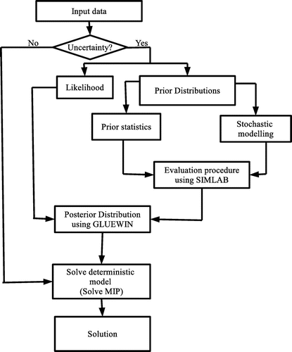
The first step is to estimate parameters that result in uncertainty with GLUE and later use the results from GLUE to solve the MIP Equations 8–14. Desalination and softening of water costs were analysed from three water sources. Means and variances were calculated after implementing MCMC method to forecast desalination and softening costs to generate more data. Normality tests were done to see if the parameters are normally distributed. Based on the results, a multivariate normal distribution was used for the desalination and softening costs. The annualised costs of desalination and softening were calculated by Equation 21 at 10% interest for the next 10 years for each new water source as predicted in the Bulawayo City Council (BCC) master plan (Bulawayo City Council, 2012). Figure 1 presents the flow chart of how GLUEMIP methodology is implemented. Water demand, annual operational costs and capital costs are input parameters that are considered to be influenced by uncertainty. We input the other parameters other than the ones mentioned in the MIP first, without using GLUE to find the mean estimates.

Figure 1. GLUEMIP flow chart.

MATLAB was used to generate N multivariate normal realisation of parameters in Table 1. Demands at node level were fitted to a uniform Dirichlet distribution which allows “string-cutting” problem formulation after using per capita demand of an individual obtained using MCMC and annual population growth forecast obtained using Equations 15–18 as $b_i={\mathit{\psi }}_i^{\ast }{N}_i^{\ast }{\mathit{\beta }}_i^{\ast }$ where ${\mathit{\psi }}_i^{\ast }$ is the sample ith component from the water allocation distribution vector, $N_i^{\ast }$ the sample from posterior predictive distribution of the population and ${\mathit{\beta }}_i^{\ast }$ sample from posterior predictive distribution of the per capita consumption. Three runs of GLUE were done to ensure that smooth posterior distributions are obtained. The likelihood value, $L(\mathit{\theta }|R)$ was computed from generated observation, R, with two replicates for each variable, for each N and for ${\mathit{\theta }}_i$, the generated parameter vector as(35) $$\begin{array}{c}\hfill L(\mathit{\theta }|R)=\prod _{j=1}^M\frac{1}{\sqrt{2\mathit{\pi }{\mathit{\sigma }}_R^2}}\exp \left(-\frac{{\left[R_j-P_j({\mathit{\theta }}_i)\right]}^2}{2{\mathit{\sigma }}_R^2}\right),i=1,2,\dots ,N\end{array}$$(35)

where ${\mathit{\theta }}_i$ is the ith parameter, $R_j$ the jth observation of R, $P_j({\mathit{\theta }}_i)$ the jth type of the model output of the set ${\mathit{\theta }}_i$, ${\mathit{\sigma }}_R^2$ the variance of model errors and M is the number of observation replicates. Mean demand is generated using Equation 19.

Table 1. Uncertainty parameters

Parameter	Resultant uncertainty parameter	unit
$d_{it}$	$d_{\mathit{\lambda }it}$	${\mathrm{m}}^3$
$e_{ijt}^u$	$e_{\mathit{\lambda }ijt}^u$	US$
$e_{ijt}^d$	$e_{\mathit{\lambda }ijt}^d$	US$
$c_{ijt}^u$	$c_{\mathit{\lambda }ijt}^u$	US$
$c_{ijt}^d$	$c_{\mathit{\lambda }ijt}^d$	US$

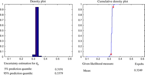
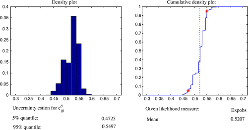
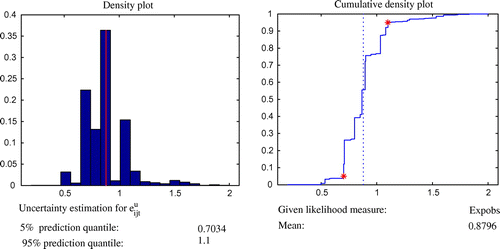
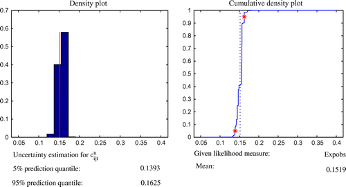
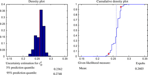
A sample of 12,413 households of different socio-economic groups was extracted from Bulawayo City Council (2006) master plan (see Table 2). Parameter sets of 100,000 were generated for each of the components, demand, $d_{it}$, annualised capital cost, $e_{ijt}^{(.)}$ and annualised operational cost, $c_{ijt}^{(.)}$, in SIMLAB 2.2.1 software. SIMLAB is a software designed to solve problems using Monte Carlo-based uncertainty and sensitivity analysis (Saltelli, 2003). SIMLAB generates samples suitable for uncertainty and sensitivity analysis of the model components. The FAST sampling method was used which was introduced by (Saltelli, Tarantola, & Chan, 1999). The predicted mean values over 1,000 runs, probability, cumulative density distributions and variance were used to characterise prediction uncertainty with 90% confidence interval in GLUEWIN (see Figures 2–6). An explanation of the GLUEWIN methodology, implementation, data requirements and analysis can be found in Ratto and Saltelli (2001). Figures 2–6 show the mean values of the five parameters and these values are the ones that are passed on to the MIP.

Figure 2. Average daily demand in $10,000{\mathrm{m}}^3$ per day.

Figure 3. Average annual capital costs of building new water plants.

Figure 4. Average annual capital costs of adding capacity to pipelines.

Figure 5. Average annual pipelines operating costs.

Figure 6. Average annual supply operating costs.

Table 2. Household water consumption data

Residential area	No. of housing units	Average household	Average household
		size	consumption (l/d)
Selbourne Park	830	6	200
Suburbs	698	6	200
Romney Park	457	7	150
Mahatshula	2,091	8	100
Sizinda	2,082	13	100
Emganwini	6,255	11	100

GLUE estimates, $d_{\mathit{\lambda }it},c_{\mathit{\lambda }ijt}^u,c_{\mathit{\lambda }ijt}^d,e_{\mathit{\lambda }ijt}^u$ and $e_{\mathit{\lambda }ijt}^d$, are then used in the main MIP. The MIP is solved in GAMS using CPlex solver. The same MIP is solved using single-point estimates of $d_{it}$, $e_{ijt}^{(.)}$ and $c_{ijt}^{(.)}$ in GAMS using CPlex solver, see Table 3 for results and parameter values that were adjusted through GLUE.

Table 3. Summary of input parameters and model results

Single-point estimate		GLUE mean estimate
Parameter	Value	Parameter	Value
$d_{it}$ (${\mathrm{m}}^3$/ day)	293,084.72	$d_{\mathit{\lambda }it}$	324,900. 56
$c_{ijt}^u$ (US$\mathrm{\$}/{\mathrm{m}}^3$ )	0.11	$c_{\mathit{\lambda }ijt}^u$	0.15
$c_{ijt}^d$ (US$\mathrm{\$}/{\mathrm{m}}^3$ )	0.18	$c_{\mathit{\lambda }ijt}^d$	0.26
$e_{ijt}^u$ (US$\mathrm{\$}/{\mathrm{m}}^3$ )	0.79	$e_{\mathit{\lambda }ijt}^u$	0.88
$e_{ijt}^d$ (US$\mathrm{\$}/{\mathrm{m}}^3$ )	0.45	$e_{\mathit{\lambda }ijt}^d$	0.52
Optimum solution (US $$/day)	178,000	Optimum solution (US $\mathrm{\$}$/ day)	201,000

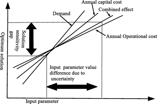
The results, in our numerical example, show a great difference in the total cost of water distribution using the two frameworks, that is, general MIP and GLUEMIP. The difference is a result of using underestimated parameter values. Usually, demand, annual capital and operational costs are underestimated if a model that does not incorporate uncertainty is used. The results are supported by that of Bunea and Bedford (2002) and Lal, Obeysekera, and van Zee (1997). The optimum solution is highly sensitive to changes in the input parameter values (see Figure 7). The other reason for the large difference, besides underestimation of input parameters, is due to the fact that the GLUEMIP uses future annual capital and operational costs, while the general MIP uses present costs. The difference is large to the extent that if water authorities do not consider uncertainties in water distribution, it can lead to serious operational challenges. The water authorities will face challenges arising from penalties for failing to meet demand.

Figure 7. Sensitivity of optimum solution to water demand, annual capital and operational costs.

Second-order dynamic linear model seems to be an efficient tool for forecasting population growth as evidenced by a large difference between point estimate demand and the demand forecast obtained using predicted population growth, which is the most influential factor of predicting demand (Polebitski & Palmer, 2010). The drawback of using the second-order DLM, coupled with normal distribution of a water consumption series, to predict future water demand, which is subject to marked changes in the regime, is that it cannot represent the time series throughout longer periods. An analysis of the second-order DLM is done for 15 years to come up with the appropriate time series. The time series is limited to 10 years and after these years, the shift in water demand seems to be exaggerated. The observation of the performance of the second-order DLM, in our results, is supported by observations of Yelland and Lee (2003), who observed the DLM’s results as compared to other forecasting techniques.

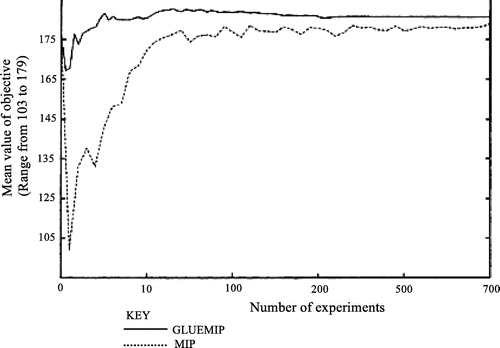
GLUEMIP proves to be a better method for forecasting future water distribution costs rather than using single-point estimates. In our results, the water authority may underestimate the costs by $23,000 and this high value slack is capable of halting the whole water resource distribution system for at least four days. GLUEMIP seems to be a significant method of finding optimal solutions of water resources management problems because it captures the important aspects in water resources management and planning. Water authorities plan for future water resource distribution aiming at meeting future water demand. The GLUEMIP methodology makes use of the important aspects of meeting future demand, that is, population growth and expansion of the water distribution networks by adjusting annual capital and operational costs. Figure 8 illustrates and compares the experiments that were carried out using different input values of water demand, annual capital and operational costs to both the GLUEMIP and general MIP. It is shown that the GLUEMIP methodology appears to be useful in optimising water resource distribution systems with uncertainties and its results are useful for better planning purposes.

Figure 8. Experimental analysis of the GLUEMIP and MIP.

4.2. Example of looped network using real data

This example uses real value data of water consumption, operational and maintenance costs. The network has 50 nodes and a total population of 1200 water consumers. The daily demand is $21,500{\mathrm{m}}^3$. The daily operational and maintenance costs are $900.00 and $575.00, respectively. The procedure of solving this problem is carried out the same way as is in Section 4.1. The results show that there is a large difference between the results obtained by MIP and that of GLUEMIP. The optimum costs, using MIP, is $72,060.00 per year, while it costs $75,700.00/ year for the same water network using GLUEMIP. Again, the water authority will underestimate the costs by $3640.00. This proves the superiority of the GLUEMIP methodology over the MIP.

5. Conclusion

GLUEMIP is a new way of incorporating uncertainty into the MIP. It seems a better way to model a water distribution network that is characterised with uncertainties arising from population growth and future operational costs. Incorporating new water sources in a water distribution network requires estimating uncertainties in pipe costs, desalination, softening and operational costs. Probability of the solution, component probabilities and the probabilities of unique sets of components can be offered through GLUEMIP output. In general, models incorporating uncertainties are preferred to deterministic models when modelling water distribution networks. The GLUEMIP results appear to be remarkably conditioned on the assumptions made in this study. Lastly, the results confirm the impact of uncertainty when optimising costs.

Additional information

Funding

The authors received no direct funding for this research.

Notes on contributors

Godfrey Chagwiza

Godfrey Chagwiza is a PhD student at National University of Science and Technology, Zimbabwe. His research interests focus on optimisation, mathematical modelling and mathematical programming.

Brian C. Jones

Brian C Jones is a professor emeritus of Applied Mathematics, National University of Science and Technology, Zimbabwe. His research interests include modelling inflow of material into black holes, as well as outflow under radiation pressure and magnetic forces, implications of spherical/cylindrical symmetries on observational parameters and protean operations research problems.

Senelani D. Hove-Musekwa

Senelani D Hove-Musekwa is an associate professor of Applied Mathematics, National University of Science and Technology, Zimbabwe. Her research interests include application of mathematics to the functioning of the human body, the interaction of the human body with infectious pathogens and the economic epidemiology.

Sobona Mtisi

Sobona Mtisi is a senior research officer, Water Policy Programme, Rural Policy and Governance Group. His research interests include socio-economic, political and institutional analyses of water resources governance.

References

- Alighanbari, M., & How, J. P. (2005). Cooperative task assignment of unmanned aerial vehicles in adversarial environments. In Proceedings Institute of Electrical and Electronics Engineers (IEEE) American Control Conference (pp. 4661–4667). Portland, OR.
- Anwar, A. A., & Clarke, D. (2001). Irrigation scheduling using mixed-integer linear programming. Journal of Irrigation and Drainage Engineering, 127, 63–69.
- Bertsimas, D., & Sim, M. (2003). Robust discrete optimization and network flows. Mathematical Programming, Series B, 98, 49–71.
- Beven, K. J., & Binley, A. M. (1992). The future of distributed models: Model calibration and uncertainty prediction. Hydrological Processes, 6, 279–298.
- Biscos, C., Mulholland, M., Le Lann, M. V., Buckley, C. A., & Brouckaert, C. J. (2003). Optimal operation of water distribution networks by predictive control using MINLP. Water SA, 29, 393–404.
- Blasone, R. S., Vrugt, J. A., Madsen, H., Rosbjerg, D., Robinson, B. A., & Zyvoloski, G. A. (2008). Generalized Likelihood Uncertainty Estimation (GLUE) using adaptive Markov chain Monte Carlo sampling. Advances in Water Resources, 31, 630–648.
- Bulawayo City Council. (2006). Water report for the period January–December 2006. Annual Water Report. Bulawayo, Zimbabwe.
- Bulawayo City Council. (2012). Water report for the period January–December 2012. Annual Water Report. Bulawayo, Zimbabwe.
- Bunea, C., & Bedford, T. (2002). The effect of model uncertainty on maintenance optimization. IEEE Transactions on Realiability, 51, 486–493.
- Cameron, D. S., Beven, K. J., & Naden, P. (2000). Flood frequency estimation by continuous simulation under climate change (with uncertainty). Hydrology and Earth System Science, 4, 393–405.
- Candela, A., Noto, L., & Aronica, G. (2005). Influence of surface roughness in hydrological response of semiarid catchments. Journal of Hydrology, 313, 119–131.
- Cembrano, G., Wells, G., Quevedo, J., Pérez, R., & Argelaguet, R. (2000). Optimal control of a water distribution network in a supervisory control system. Control Engineering Practice, 8, 1177–1188.
- Chow, N. H. (1995). A study on optimal management of water resources in Kaoping area Taiwan(I). In Project Completion Representation to National Science Council. Taipei, Taiwan, R.O.C.
- Creasey, J. D. (1988). Pump scheduling in water supply: More than a mathematical problem. In B. Coulbeck & C. H. Orr (Eds.), Computer application in water supply. Systems optimization and control. (Vol. 2, pp. 279–289). Taunton: Research Studies Press Ltd.
- de Vries, T. T., & Anwar, A. A. (2004). Irrigation scheduling 1: Integer programming approach. Journal of Irrigation and Drainage Engineering, 130, 9–16.
- Dye, S., Stougle, L., & Tomasgard, A. (2003). The stochastic single resource service-provision problem. Naval Research Logistics, 50, 869–887.
- Freni, G., Mannina, G., & Viviani, G. (2009). Assessment of data availability influence on integrated urban drainage modelling uncertainty. Environment Model Software, 24, 1171–1181.
- Garey, M. R., & Johnson, D. S. (1979). Computers and intractability: A guide to the theory of NP-completeness. New York, NY: WH Freeman and Company.
- Garfinkel, R. S., & Nemhauser, G. L. (1972). Integer programming (2nd ed.). New York, NY: John Wiley.
- Gelman, A., Carlin, J. B., Stren, H. S., & Rubin, D. B. (1995). Bayesian data analysis. New York, NY: Chapmann and Hall.
- Gonen, T., & Foote, B. L. (1981). Distribution system planning using mixed-integer programming. Generation, Transmission and Distribution, IEEE Conference, 128, 70–79.
- Gurkan, G., Ozge, A. Y., & Robinson, S. M. (1999). Solving stochastic optimization problems with stochastic constraints: An application in network design. In P. A. Farrington, H. B. Nembhard, D. T. Sturrock, & G. W. Evans (Eds.), Proceedings of the 1999 Winter Simulation Conference (pp. 471–478). Washington, DC: Omnipress.
- Kallrath, J., & Wilson, J. M. (1997). Business optimisation using mathematical programming. London: Macmillan.
- Lal, W., Obeysekera, J., & van Zee, R. (1997). Sensitivity and uncertainty analysis of a regional simulation model for the natural system in South Florida. In Managing water: Coping with scarcity and abundance. San Francisco, CA.
- Madden, C., & Carmichael, A. (2007). Every last drop. Sydney: Random House Australia.
- Makowski, D., Wallach, D., & Tremblay, M. (2002). Using a bayesian approach to parameter estimation: Comparison of the glue and mcmc methods. Agronomie, 22, 191–203.
- Mannina, G. (2005). Integrated urban drainage modelling with uncertainty for stormwater pollution management (PhD thesis). Universita di Catania, Italy.
- Polebitski, A. & Palmer, R. (2010). Seasonal residential water demand forecasting for census tracts. Journal of Water Resources Planning and Management, 136, 27–36.
- Ramesh, B. R., Venugopal, K., & Karunakaran, K. (2009). Zero-one programming model for daily operation scheduling for irrigation canal. Journal of Agricultural Science, 1, 13–20.
- Ratto, M., & Saltelli, A. (2001). Model assessment in integrated procedures for environmental impact evaluation: Software prototypes. IMPACT project, deliverable 18, Joint Research Centre of European Commission, Institute for the Protection and Security of the Citizen. Ispra.
- Refsgaard, J. P., Van der Sluijs, J. P., Højberg, A. L., & Vanrolleghem, P. A. (2007). Uncertainty in the environmental modelling process—A framework and guidance. Environment Model Software, 22, 1543–1556.
- Romanowicz, R. & Beven, K. J. (1998). Dynamic real-time prediction of flood inundation probabilities. Hydrology Science Journal, 43, 181–196.
- Saltelli, A. (2003). SIMLAB 2.2 manual, simulation environment for uncertainty and sensitivity analysis. SIMLAB 2.2 Manual, JRC/ POLIS ScaRL, SIMLAB.
- Saltelli, A., Tarantola, S., & Chan, K. P. S. (1999). A quantitative model-independent method for global sensitivity analysis of model output. Technometrics, 41, 39–56.
- Sandholm, T., Gilpin, A., & Conitzer, V. (2005). Mixed-integer programming methods for finding Nash equilibria. American Association for Artificial Intelligence (AAAI)-05, National Conference on Artifcial Intelligence (pp. 495–501). Pennsylvania: Pittsburgh.
- Sen, S. & Higle, J. L. (1999). An introductory tutorial on stochastic linear programming models. Interfaces, 29, 33–61.
- Smith, J. C., & Taskin, Z. C. (2008). A tutorial guide to mixed-integer programming models and solution techniques. In G. J. Lim & E. K. Lee (Eds.), Optimization in Medicine and Biology. Auerbach Publications: Taylor and Francis.
- Suryavanshi, A. R. & Reddy, J. M. (1986). Optimal operation schedule of irrigation distribution systems. Agricultural Water Management, 11, 23–30.
- von Bertalanffy, L. (1968). General system theory. New York, NY: Braziller.
- Vossen, T., Ball, M., & Smith, R. H. (1999). On the use of integer programming models in AI planning. In Sixth International Joint Conference on Artificial Intelligence (IJCAI)-99 (pp. 304–309). San Francisco, CA; Morgan Kaufmann.
- West, M., & Harrison, J. (1997). Bayesian forecasting and dynamic models. Springer series in statistics (2nd ed.). New York, NY: Springer-Verlag.
- Willems, P. (2000). Quantification and relative comparison of different types of uncertainties in sewer water quality modelling. Water Research, 42, 3539–3551.
- Williams, H. P. (1993). Model building in mathematical programming (3rd ed.). Chichester: John Wiley.
- Yelland, P. M., & Lee, E. (2003). Forecasting product sales with dynamic linear mixture models. SMLI TR-2003-122. Sun Microsystems Inc., Mountain View, CA.