Dissipativity and passivity analysis for discrete-time complex-valued neural networks with time-varying delay

Abstract

In this paper, we consider the problem of dissipativity and passivity analysis for complex-valued discrete-time neural networks with time-varying delays. The neural network under consideration is subject to time-varying. Based on an appropriate Lyapunov–Krasovskii functional and by using the latest free-weighting matrix method, a sufficient condition is established to ensure that the neural networks under consideration is strictly $(\mathcal{Q},\mathcal{S},\mathcal{R})$-dissipative. The derived conditions are presented in terms of linear matrix inequalities. A numerical example is presented to illustrate the effectiveness of the proposed results.

Keywords:

• complex-valued neural networks
• dissipativity
• Lyapunov–Krasovskii functional
• linear matrix inequalities(LMIs)
• time-varying delay

Public Interest Statement

The passivity approach for interconnection of passive systems provides a nice tool for controlling a large class of nonlinear systems and DNNs, and its potential applications have been found in the stability and stabilization schemes of electrical networks, and in the control of teleoperators.

1. Introduction

In the past several decades, the neural networks are very important nonlinear circuit networks because of their wide applications in various fields such as associative memory, signal processing, data compression, system control (Hirose, 2003), optimization problem, and so on Liang, Wang, and Liu (2009), Wang, Ho, Liu, and Liu (2009), Liu, Wang, Liang, and Liu (2009), Bastinec, Diblik, and Smarda (2010), and Diblik, Schmeidel, and Ruzickova (2010). Recently, neural networks have been electronically implemented and they have been used in real-time applications. However in electronic implementation of neural networks, some essential parameters of neural networks such as release rate of neurons, connection weights between the neurons and transmission delays might be subject to some deviations due to the tolerances of electronic components employed in the design of neural networks (Aizenberg, Paliy, Zurada, & Astola, 2008; Hu & Wang, 2012; Mostafa, Teich, & Lindner, 2013; Wang, Xue, Fei, & Li, 2013; Wu, Shi, Su, & Chu, 2011). As we know, time delays commonly exist in the neural networks because of the network traffic congestions and the finite speed of information transmission in networks. So the study of dynamic properties with time delay is of great significance and importance. However, most of the studied networks are real number valued. Recently, in order to investigate the complex properties in complex-valued neural networks, some complex-valued network models are proposed.

Figure 1. State trajectories of real part of two-neuron complex-valued neural networks for ${\mathit{\tau }}_1(k)=2.5+0.5sin(0.5k\mathit{\pi })$ and ${\mathit{\tau }}_2(k)=4.5+0.5sin(0.5k\mathit{\pi })$ with initial states $x_{11}=2+2j$.

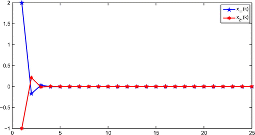
Figure 2. State trajectories of imaginary part of two-neuron complex-valued neural networks for ${\mathit{\tau }}_1(k)=2.5+0.5sin(0.5k\mathit{\pi })$ and ${\mathit{\tau }}_2(k)=4.5+0.5sin(0.5k\mathit{\pi })$ with initial states $x_{12}=-1-j$.

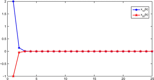
Figure 3. State trajectories of real part of two-neuron complex-valued neural networks for ${\mathit{\tau }}_1(k)=3.5+0.5sin(0.5k\mathit{\pi })$ and ${\mathit{\tau }}_2(k)=5.5+0.5sin(0.5k\mathit{\pi })$ with initial states $x_{11}=2+2j$.

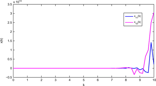
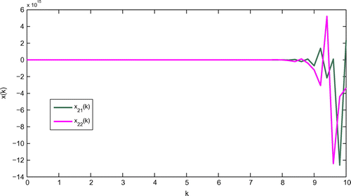
Figure 4. State trajectories of imaginary part of two-neuron complex-valued neural networks for ${\mathit{\tau }}_1(k)=3.5+0.5sin(0.5k\mathit{\pi })$ and ${\mathit{\tau }}_2(k)=5.5+0.5sin(0.5k\mathit{\pi })$ with initial states $x_{12}=-1-j$.

The most notable feature of complex-valued neural networks (CVNNs) is the compatibility with wave phenomena and wave information related to, for example, electromagnetic wave, light wave, electron wave, and sonic wave (Hirose, 2011). Furthermore, CVNNs are widely applied in coherent electromagnetic wave signal processing. They are mainly used in adapting, processing of interferometric synthetic aperture radar (InSAR) images captured by satellite or airplane to observe land surface (Suksmono & Hirose, 2002; Yamaki & Hirose 2009). Another important application field is sonic and ultrasonic processing. Pioneering work has been done in various directions (Zhang & Ma, 1997). In communication systems, the CVNNS can be regarded as an extension of adaptive complex filters, i.e. modular multiple-stage and nonlinear version. From this view point, several groups worked on time sequential signal processing (Goh & Mandic, 2007, 2005). Furthermore, there are many ideas based on CVNNs in image processing. An example is the adaptive processing for blur compensation by identifying the point scatting function in the frequency domain (Aizenberg et al., 2008). Recently, many mathematicians and scientists have paid more attention to this field of research. Besides, CVNNs have different and more complicated properties than the real-valued ones. Therefore, it is necessary to study the dynamic behaviors of the systems deeply. Over the past decades, some work has been done to analyze the dynamic behavior of the equilibrium points of the various CVNNs. In Mostafa et al. (2013), local stability analysis of discrete-time, continuous-state, complex-valued recurrent neural networks with inner state feedback was presented. In Zhou and Song (2013), the authors studied boundedness and complete stability of complex-valued neural networks with time delay by using free weighting matrices.

It is well known that dissipativity theory gives a framework for the design and analysis of control systems using an input?output description on energy-related considerations (Jing, Yao, & Shen, 2014; Wu, Shi, Su, & Chu, 2013; Wu, Yang, & Lam, 2014) and it becomes a powerful tool in characterizing important system behaviors such as stability. The passivity theory, being an effective tool for analyzing the stability of systems, has been applied in complexity (Zhao, Song, & He, 2014), signal processing, especially for high-order systems and thus the passivity analysis approach has been used for a long time to deal with the control problems (Chua, 1999). However, to the best of our knowledge, there is no result addressed on the dissipativity and passivity analysis of discrete-time complex-valued neural networks with time-varying delay, which motivates the present study.

In this paper, we consider the problem of dissipativity and passivity analysis for discrete-time complex-valued neural networks with time-varying delay. Based on the lemma proposed in Zhou and Song (2013), a condition is derived for strict $(\mathcal{Q},\mathcal{S},\mathcal{R})$-dissipativity and passivity of the control neural networks, which depends only on the discrete delay. In established model, the delay-dependent dissipativity and passivity conditions are derived and the obtained linear matrix inequalities (LMIs) can be checked numerically using the effective LMI toolbox in MATLAB and accordingly the estimator gains are obtained. The effectiveness of the proposed design is finally demonstrated by a numerical example.

The rest of this paper is organized as follows: model description and preliminaries are given in Section 2. Dissipativity and passivity analysis for discrete-time complex-valued neural networks with time-varying delay are presented in Section 3. Illustrative example and its simulation results for dissipativity conditions have been given in Section 4.

Notations: ${\mathbb{C}}^n$ and ${\mathbb{R}}^n$ denote, respectively, the $n$-dimensional complex space and Euclidean space. $z(k)=x(k)+iy(k)$ denote the complex-valued function, where $x(k)$, $y(k)\in {\mathbb{R}}^n$. ${\mathbb{R}}^{n\times m}$ is the set of real $n\times m$ matrices, $I$ is the identity matrix of appropriate dimension. For any matrix $P$, $P>0$$(P<0)$ means $P$ is a positive definite (negative definite) matrix. The superscript $\ast$ denotes the matrix complex conjugate transpose, $diag\{···\}$ stands for a block-diagonal matrix. Let $\mathcal{C}([-{\mathit{\tau }}_2,0],\mathcal{D})$ be the Banach space of continuous functions mapping $[-{\mathit{\tau }}_2,0]$ into $\mathcal{D}\subset {\mathbb{C}}^n$. For integers $a$ and $b$ with $a<b$, let $N[a,b]=a,a+1,\dots ,b-1,b$. $X^T$ represents the transpose of matrix $X$, $\mathrm{\Delta }V(k)$ denotes the difference of function $V(k)$ given by $\mathrm{\Delta }V(k)=V(k+1)-V(k).$

2. Model description and preliminaries

Consider the following discrete-time complex-valued neural networks with time-varying delays:(1) $$\begin{array}{cc}\hfill z(k+1)& =Af(z(k))+Bf(z(k-\mathit{\tau }(k)))+u(k)\hfill \\ \hfill \mathit{y}(k)& =f(z(k))\hfill \end{array}$$(1)

where $z(k)={[z_1(k),z_2(k),\dots z_n(k)]}^T\in {\mathbb{C}}^n$ is the neuron state vector; $A\in {\mathbb{C}}^{n\times n}$, $B\in {\mathbb{C}}^{n\times n}$ are the connection weight matrix and the delayed connection weight matrix, respectively; $y(k)$ is the output of neural network (1). $u(k)={[u_1(k),u_2(k),\dots u_n(k)]}^T\in {\mathbb{C}}^n$ is the input vector; time delay $\mathit{\tau }(k)$ ranges from ${\mathit{\tau }}_1$ to ${\mathit{\tau }}_2$ as ${\mathit{\tau }}_1\le \mathit{\tau }(k)\le {\mathit{\tau }}_2$; $f(z(k))={[f_1(z_1(k)),\dots ,f_n(z_n(k))]}^T\in {\mathbb{C}}^n$ and $f(z(k-\mathit{\tau }(k)))={[f_1(z_1(k-{\mathit{\tau }}_1(k))),\dots ,f_n(z(k-{\mathit{\tau }}_1(k)))]}^T\in {\mathbb{C}}^n$ are the complex-valued neuron activation functions without and with time delays. The initial conditions of the CVNNs (1) are given by$$\begin{array}{c}\hfill z_i(s)={\mathit{\varphi }}_i(s),s\in [-{\mathit{\tau }}_2,0],i=1,2,\dots ,n\end{array}$$

where ${\mathit{\varphi }}_i\in \mathcal{C}([-{\mathit{\tau }}_2,0],\mathcal{D})$ are continuous. Complex-valued parameters in the neural network can be represented as $a_{ij}=a_{ij}^R+i{a}_{ij}^I$, $b_{ij}=b_{ij}^R+i{b}_{ij}^I$. Then (1) can be written as(2) $$\begin{array}{cc}\hfill z_i^R(k+1)& =\sum _{j=1}^n{a}_{ij}^{R}f(z_j^R(k))-\sum _{j=1}^n{a}_{ij}^{I}f(z_j^I(k))+\sum _{j=1}^n{b}_{ij}^{R}f(z_j^R(k-\mathit{\tau }(k)))-\sum _{j=1}^n{b}_{ij}^{I}f(z_j^I(k-\mathit{\tau }(k)))\hfill \\ \hfill & +u_i^R(k)\hfill \\ \hfill z_i^I(k+1)& =\sum _{j=1}^n{a}_{ij}^{R}f(z_j^I(k))+\sum _{j=1}^n{a}_{ij}^{I}f(z_j^R(k))+\sum _{j=1}^n{b}_{ij}^{R}f(z_j^I(k-\mathit{\tau }(k)))+\sum _{j=1}^n{b}_{ij}^{I}f(z_j^R(k-\mathit{\tau }(k)))\hfill \\ \hfill & +u_i^I(k)\hfill \end{array}$$(2)

where $z_i^R$ and $z_i^I$ are the real and imaginary parts of variable $z_i$, respectively. $a_{ij}^R$ and $a_{ij}^I$ are the real and imaginary parts of connection weight $a_{ij}$; $b_{ij}^R$ and $b_{ij}^I$ are the real and imaginary parts of delayed connection weight $b_{ij}$. $u_i^R(k)$ and $u_i^I(k)$ are the real and imaginary parts of $u(k)$. Connection weight matrices are represented as $A^R={(a_{ij}^R)}_{n\times n}\in {\mathbb{R}}^{n\times n}$, $A^I={(a_{ij}^I)}_{n\times n}\in {\mathbb{R}}^{n\times n}$, $B^R={(b_{ij}^R)}_{n\times n}\in {\mathbb{R}}^{n\times n}$, and $B^I={(b_{ij}^I)}_{n\times n}\in {\mathbb{R}}^{n\times n}$. Then, we have$$\begin{array}{cc}\hfill z^R(k+1)& =A^R{f}^R(k)-A^I{f}^I(k)+B^R{f}^R(k-\mathit{\tau }(k)))-B^I{f}^I(k-\mathit{\tau }(k)))+u^R(k)\hfill \\ \hfill z^I(k+1)& =A^R{f}^I(k)+A^I{f}^R(k)+B^R{f}^I(k-\mathit{\tau }(k)))+B^I{f}^R(k-\mathit{\tau }(k)))+u^I(k)\hfill \end{array}$$

To derive the main results, we will introduce the following assumptions, definitions, and lemmas.

Assumption 2.1

The activation function $f_j(·)$ can be separated into real and imaginary parts of the complex numbers $z$. It follows that $f_j(z)$ is expressed by$$\begin{array}{c}\hfill f_j(z)=f_j^R(Re(z))+i{f}_j^I(Im(z))\end{array}$$

where $f_i^R(·)$, $f_j^I(·):\mathbb{R}\to \mathbb{R}$ for all $j=1,2,\dots ,n$. Then,$$\begin{array}{c}\hfill l_j^{R-}\le \frac{f_j^R({\mathit{\alpha }}_1)-f_j^R({\mathit{\alpha }}_2)}{{\mathit{\alpha }}_1-{\mathit{\alpha }}_2}\le l_j^{R+}\end{array}$$$$\begin{array}{c}\hfill l_j^{I-}\le \frac{f_j^I({\mathit{\alpha }}_1)-f_j^I({\mathit{\alpha }}_2)}{{\mathit{\alpha }}_1-{\mathit{\alpha }}_2}\le l_j^{I+},\forall {\mathit{\alpha }}_1,{\mathit{\alpha }}_2\in \mathbb{R},{\mathit{\alpha }}_1\ne {\mathit{\alpha }}_2\end{array}$$

Definition 2.1

Zhou and Song (2013): The neural network (1) is said to be $(\mathcal{Q},S,R)$-dissipative, if the following dissipation inequality(3) $$\begin{array}{c}\hfill \sum _{k=0}^{k_p}r(u(k),y(k))\ge 0,\forall k_p\ge 0\end{array}$$(3)

holds under zero initial condition for any nonzero input $u\in l_2[0,+\infty )$. Furthermore, if for some scalar $\mathit{\gamma }>0$, the dissipation inequality(4) $$\begin{array}{c}\hfill \sum _{k=0}^{k_p}r(u(k),y(k))\ge \mathit{\gamma }\sum _{k=0}^{k_p}{u}^T(k)u(k)\forall k_p\ge 0\end{array}$$(4)

holds under zero initial condition for any nonzero input $u\in l_2[0,+\infty )$, then the neural network (1) is said to be strictly $(\mathcal{Q},S,R)$-$\mathit{\gamma }$-dissipative. In this paper, we define a quadratic supply rate $r(u,y)$ associated with neural network (1) as follows:(5) $$\begin{array}{c}\hfill r(u,y)=y^T\mathcal{Q}y+2y^T\mathcal{S}u+u^T\mathcal{R}u\end{array}$$(5)

where $\mathcal{Q}\le 0$, $\mathcal{S}$, and $\mathcal{R}$ are real symmetric matrices of appropriate dimensions.

Definition 2.2

Wu et al. (2011): The neural network (1) is said to be passive if there exists a scalar $\mathit{\gamma }>0$ such that, for all $k_0\ge 0$$$\begin{array}{c}\hfill 2\sum _{j=0}^{k_0}{y}^T(j)u(j)\ge -\mathit{\gamma }\sum _{j=0}^{k_0}{u}^T(j)u(j)\end{array}$$

under the zero initial condition.

Lemma 2.1

Liu et al. (2009): Let $X$ and $Y$ be any $n$-dimensional real vectors, and let $P$ be an $n\times n$ positive semidefinite matrix. Then, the following inequality holds:$$\begin{array}{c}\hfill 2X^{T}PY\le X^{T}PX+Y^{T}PY\end{array}$$

Lemma 2.2

For any constant matrix $M\in {\mathbb{R}}^{n\times n}$, $M=M^T>0$, integers $r_1$ and $r_2$ satisfying $r_2>r_1$, and vector function $\mathit{\omega }:\mathbb{N}[r_1,r_2]\to {\mathbb{R}}^n$, such that the sums concerned are well defined, then(6) $$\begin{array}{c}\hfill -(r_2-r_1+1)\sum _{j=r_1}^{r_2}{\mathit{\omega }}^T(j)M\mathit{\omega }(j)\le -\sum _{j=r_1}^{r_2}{\mathit{\omega }}^T(j)M\sum _{j=r_1}^{r_2}\mathit{\omega }(j)\end{array}$$(6)

Proof

$$\begin{array}{cc}\hfill -(r_2-r_1+1)\sum _{j=r_1}^{r_2}{\mathit{\omega }}^T(j)M\mathit{\omega }(j)& =-\frac{1}{2}(r_2-r_1+1)\sum _{j=r_1}^{r_2}{\mathit{\omega }}^T(j)M\mathit{\omega }(j)-\frac{1}{2}(r_2-r_1+1)\sum _{j=r_1}^{r_2}{\mathit{\omega }}^T(j)M\mathit{\omega }(j)\hfill \\ \hfill & =-\frac{1}{2}(r_2-r_1+1)\sum _{i=r_1}^{r_2}{\mathit{\omega }}^T(i)M\mathit{\omega }(i)-\frac{1}{2}(r_2-r_1+1)\sum _{j=r_1}^{r_2}{\mathit{\omega }}^T(j)M\mathit{\omega }(j)\hfill \\ \hfill & =-\frac{1}{2}[\sum _{i=r_1}^{r_2}(r_2-r_1+1){\mathit{\omega }}^T(i)M\mathit{\omega }(i)+\sum _{i=r_1}^{r_2}\sum _{j=r_1}^{r_2}{\mathit{\omega }}^T(j)M\mathit{\omega }(j)]\hfill \\ \hfill & =-\frac{1}{2}\sum _{j=r_1}^{r_2}[(r_2-r_1+1){\mathit{\omega }}^T(i)M\mathit{\omega }(i)+\sum _{j=r_1}^{r_2}{\mathit{\omega }}^T(j)M\mathit{\omega }(j)]\hfill \\ \hfill & =-\frac{1}{2}\sum _{j=r_1}^{r_2}\sum _{j=r_1}^{r_2}[{\mathit{\omega }}^T(j)M\mathit{\omega }(j)+{\mathit{\omega }}^T(i)M\mathit{\omega }(i)]\hfill \\ \hfill & \le -\sum _{j=r_1}^{r_2}\sum _{i=r_1}^{r_2}{\mathit{\omega }}^T(j)M\mathit{\omega }(i)[UsingLemma2.1]\hfill \\ \hfill & =-\sum _{j=r_1}^{r_2}{\mathit{\omega }}^T(j)M\sum _{i=r_1}^{r_2}\mathit{\omega }(i)\hfill \\ \hfill \end{array}$$

Lemma 2.3

Let $M\in {\mathbb{R}}^{n\times n}$ be a positive semidefinite matrix, ${\mathit{\xi }}_j\in {\mathbb{R}}^n$, and scalar constant $a_j\ge 0$$(j=1,2,\dots )$. If the series concerned is convergent, then the following inequality holds:(7) $$\begin{array}{c}\hfill (\sum _{j=1}^{\infty }{a}_j{\mathit{\xi }}_j{)}^{T}M(\sum _{j=1}^{\infty }{a}_j{\mathit{\xi }}_j)\le (\sum _{j=1}^{\infty }{a}_j)\sum _{j=1}^{\infty }{a}_j{\mathit{\xi }}_j^{T}M{\mathit{\xi }}_j\end{array}$$(7)

Proof

Letting m be a positive integer, we have$$\begin{array}{cc}\hfill (\sum _{j=1}^m{a}_j{\mathit{\xi }}_j{)}^{T}M(\sum _{j=1}^m{a}_j{\mathit{\xi }}_j)& =(\sum _{j=1}^m{a}_j{\mathit{\xi }}_j{)}^{T}M(\sum _{i=1}^m{a}_i{\mathit{\xi }}_i)\hfill \\ \hfill & =\sum _{j=1}^m\sum _{i=1}^m{a}_j{a}_i{\mathit{\xi }}_j^{T}M{\mathit{\xi }}_i\hfill \\ \hfill & \le \sum _{j=1}^m\sum _{i=1}^m\frac{1}{2}{a}_j{a}_i({\mathit{\xi }}_j^{T}M{\mathit{\xi }}_j+{\mathit{\xi }}_i^{T}M{\mathit{\xi }}_i)(bytheLemma2.1)\hfill \\ \hfill & =(\sum _{j=1}^m{a}_j)\sum _{j=1}^m{a}_j{\mathit{\xi }}_j^{T}M{\mathit{\xi }}_j\hfill \end{array}$$

and then (8) follows directly by letting $m\to \infty$, which completes the proof.

Lemma 2.4

Given a Hermitian matrix $Q$, The inequality $Q<0$ is equivalent to$$\begin{array}{c}\hfill \left(\begin{array}{cc}{\mathbb{Q}}^R& -{\mathbb{Q}}^I\\ {\mathbb{Q}}^I& {\mathbb{Q}}^R\end{array}\right)<0\end{array}$$

where ${\mathbb{Q}}^R=Re(\mathbb{Q})$ and ${\mathbb{Q}}^I=Im(\mathbb{Q})$.

3. Main results

In this section, we derive the dissipativity criterion for discrete-time complex-valued neural networks (1) with time-varying delays using the Lyapunov functional method combining with LMI approach. For convenience, we use the following notations: $\mathit{\psi }(k)=\frac{1}{\mathit{\alpha }(k)}[{\sum }_{i=k-\mathit{\tau }(k)}^{k-{\mathit{\tau }}_1-1}z(i)],$$\mathit{\varphi }(k)=\frac{1}{\mathit{\beta }(k)}[{\sum }_{i=k-{\mathit{\tau }}_2}^{k-\mathit{\tau }(k)-1}z(i)],$$M=\frac{{\mathit{\tau }}_1^4}{4}G+\frac{{({\mathit{\tau }}_2-{\mathit{\tau }}_1)}^2}{4}H,$$\mathit{\alpha }(k)=\mathit{\tau }(k)-{\mathit{\tau }}_1,$$\mathit{\beta }(k)={\mathit{\tau }}_2-\mathit{\tau }(k)$. Table 1 describes the matrices along with the dimensions that are used in the following Theorem 3.1.

Theorem 3.1

Assume that Assumption 2.1 holds, then the complex-valued neural networks (1) are dissipative if there exist positive Hermitian matrices $P=P_1+i{P}_2$, $Q=Q_1+i{Q}_2$, $R=R_1+i{R}_2$, $S=S_1+i{S}_2$, $T=T_1+i{T}_2$, $U=U_1+i{U}_2$, $V=V_1+i{V}_2$, $W=W_1+i{W}_2$, $G=G_1+i{G}_2$, $H=H_1+i{H}_2$, two positive diagonal matrices $F_1>0$, $F_2>0$, and a scalar $\mathit{\gamma }>0$ such that the following LMI holds.(8) $$\begin{array}{c}\hfill \mathrm{\Theta }=\left(\begin{array}{cc}{\mathrm{\Theta }}^R& -{\mathrm{\Theta }}^I\\ {\mathrm{\Theta }}^I& {\mathrm{\Theta }}^R\end{array}\right)<0\end{array}$$(8)

where(9) $$\begin{array}{c}\hfill {\mathrm{\Theta }}^R=\left(\begin{array}{ccccccccccc}{\mathrm{\Theta }}_{1,1}^R& 0& 0& 0& {\mathrm{\Theta }}_{1,5}^R& {\mathrm{\Theta }}_{1,6}^R& {\mathrm{\Theta }}_{1,7}^R& 0& 0& 0& {\mathrm{\Theta }}_{1,11}^R\\ 0& {\mathrm{\Theta }}_{2,2}^R& 0& 0& 0& 0& 0& 0& {\mathrm{\Theta }}_{2,9}^R& 0& 0\\ 0& 0& {\mathrm{\Theta }}_{3,3}^R& 0& 0& 0& 0& 0& {\mathrm{\Theta }}_{3,9}^R& 0& 0\\ 0& 0& 0& {\mathrm{\Theta }}_{4,4}^R& 0& 0& 0& 0& 0& 0& 0\\ 0& 0& 0& 0& {\mathrm{\Theta }}_{5,5}^R& {\mathrm{\Theta }}_{5,6}^R& 0& 0& 0& 0& {\mathrm{\Theta }}_{5,11}^R\\ 0& 0& 0& 0& 0& {\mathrm{\Theta }}_{6,6}^R& 0& 0& 0& 0& {\mathrm{\Theta }}_{6,11}^R\\ 0& 0& 0& 0& 0& 0& {\mathrm{\Theta }}_{7,7}^R& 0& 0& 0& 0\\ 0& 0& 0& 0& 0& 0& 0& {\mathrm{\Theta }}_{8,8}^R& 0& 0& 0\\ 0& 0& 0& 0& 0& 0& 0& 0& {\mathrm{\Theta }}_{9,9}^R& 0& 0\\ 0& 0& 0& 0& 0& 0& 0& 0& 0& {\mathrm{\Theta }}_{10,10}^R& 0\\ 0& 0& 0& 0& 0& 0& 0& 0& 0& 0& {\mathrm{\Theta }}_{11,11}^R\end{array}\right)\end{array}$$(9)

and(10) $$\begin{array}{c}\hfill {\mathrm{\Theta }}^I=\left(\begin{array}{ccccccccccc}{\mathrm{\Theta }}_{1,1}^I& 0& 0& 0& {\mathrm{\Theta }}_{1,5}^I& {\mathrm{\Theta }}_{1,6}^I& {\mathrm{\Theta }}_{1,7}^I& 0& 0& 0& {\mathrm{\Theta }}_{1,11}^I\\ 0& {\mathrm{\Theta }}_{2,2}^I& 0& 0& 0& 0& 0& 0& {\mathrm{\Theta }}_{2,9}^I& 0& 0\\ 0& 0& {\mathrm{\Theta }}_{3,3}^I& 0& 0& 0& 0& 0& {\mathrm{\Theta }}_{3,9}^I& 0& 0\\ 0& 0& 0& {\mathrm{\Theta }}_{4,4}^I& 0& 0& 0& 0& 0& 0& 0\\ 0& 0& 0& 0& {\mathrm{\Theta }}_{5,5}^I& {\mathrm{\Theta }}_{5,6}^I& 0& 0& 0& 0& {\mathrm{\Theta }}_{5,11}^I\\ 0& 0& 0& 0& 0& {\mathrm{\Theta }}_{6,6}^I& 0& 0& 0& 0& {\mathrm{\Theta }}_{6,11}^I\\ 0& 0& 0& 0& 0& 0& {\mathrm{\Theta }}_{7,7}^I& 0& 0& 0& 0\\ 0& 0& 0& 0& 0& 0& 0& {\mathrm{\Theta }}_{8,8}^I& 0& 0& 0\\ 0& 0& 0& 0& 0& 0& 0& 0& {\mathrm{\Theta }}_{9,9}^I& 0& 0\\ 0& 0& 0& 0& 0& 0& 0& 0& 0& {\mathrm{\Theta }}_{10,10}^I& 0\\ 0& 0& 0& 0& 0& 0& 0& 0& 0& 0& {\mathrm{\Theta }}_{11,11}^I\end{array}\right)\end{array}$$(10)

with$$\begin{array}{cc}\hfill {\mathrm{\Theta }}_{1,1}^R& =-P_1+Q_1+R_1+T_1+{\mathit{\tau }}_1^2{U}_1+{\mathit{\tau }}_2^2{V}_1+M_1-{\mathit{\tau }}_1^2{G}_1+F_1\mathrm{\Gamma }\hfill \\ \hfill {\mathrm{\Theta }}_{1,5}^R& =-A_1^T{M}_1-A_2^T{M}_2,{\mathrm{\Theta }}_{1,6}^R=-B_1^T{M}_1-B_2^T{M}_2,{\mathrm{\Theta }}_{1,7}^R=-{\mathit{\tau }}_1{G}_1,{\mathrm{\Theta }}_{1,11}^R=-M_1\hfill \\ \hfill {\mathrm{\Theta }}_{2,2}^R& =-Q_1+S_1-H_1,{\mathrm{\Theta }}_{2,9}^R=H_1,{\mathrm{\Theta }}_{3,3}^R=-H_1-R_1-S_1,{\mathrm{\Theta }}_{3,9}^R=H_1\hfill \\ \hfill {\mathrm{\Theta }}_{4,4}^R& =-T_1+B_1^T{P}_1{B}_1-B_1^T{P}_2{B}_2+B_2^T{P}_2{B}_1+B_2^T{P}_1{B}_2-F_2\mathrm{\Gamma }\hfill \\ \hfill {\mathrm{\Theta }}_{5,5}^R& =A_1^T{P}_1{A}_1-A_1^T{P}_2{A}_2+A_2^T{P}_2{A}_1+A_2^T{P}_1{A}_2+A_1^T{M}_1{A}_1-A_1^T{M}_2{A}_2+A_2^T{M}_2{A}_1\hfill \\ \hfill & +A_2^T{M}_1{A}_2-{\mathcal{Q}}_1-F_1,{\mathrm{\Theta }}_{5,6}^R=A_1^T{P}_1{B}_1-A_1^T{P}_2{B}_2+A_2^T{P}_2{B}_1+A_2^T{P}_1{B}_2\hfill \\ \hfill {\mathrm{\Theta }}_{5,11}^R& =P_1{A}_1-P_2{A}_2+M_1{A}_1-M_2{A}_2-I-{\mathcal{S}}_1\hfill \\ \hfill {\mathrm{\Theta }}_{6,6}^R& =B_1^T{M}_1{B}_1-B_1^T{M}_2{B}_2+B_2^T{M}_2{B}_1+B_2^T{P}_1{B}_2-F_2,{\mathrm{\Theta }}_{6,11}^R=B_1^T{P}_1+B_2^T{P}_2\hfill \\ \hfill {\mathrm{\Theta }}_{7,7}^R& =-U_1+G_1,{\mathrm{\Theta }}_{8,8}^R=-V_1,{\mathrm{\Theta }}_{9,9}^R=-H_1,{\mathrm{\Theta }}_{10,10}^R=-H_1,{\mathrm{\Theta }}_{11,11}^R=-{\mathcal{R}}_1+\mathit{\gamma }I+P_1{M}_1\hfill \\ \hfill {\mathrm{\Theta }}_{1,1}^I& =-P_1+Q_1+R_1+T_1+{\mathit{\tau }}_1^2{U}_1+{\mathit{\tau }}_2^2{V}_1+M_1-{\mathit{\tau }}_1^2{G}_1\hfill \\ \hfill {\mathrm{\Theta }}_{1,5}^I& =-A_1^T{M}_2-A_2^T{M}_1,{\mathrm{\Theta }}_{1,6}^I=-B_1^T{M}_2-B_2^T{M}_1,{\mathrm{\Theta }}_{1,7}^I=-{\mathit{\tau }}_1{G}_2,{\mathrm{\Theta }}_{1,11}^I=-M_2\hfill \\ \hfill {\mathrm{\Theta }}_{2,2}^I& =-Q_2+S_2-H_2,{\mathrm{\Theta }}_{2,9}^I=H_2,{\mathrm{\Theta }}_{3,3}^I=-H_2-R_2-S_2,{\mathrm{\Theta }}_{3,9}^I=H_2\hfill \\ \hfill {\mathrm{\Theta }}_{4,4}^I& =-T_2+B_1^T{P}_2{A}_1+B_1^T{P}_1{B}_2-B_2^T{P}_1{B}_1+B_2^T{P}_2{B}_2\hfill \\ \hfill {\mathrm{\Theta }}_{5,5}^I& =A_1^T{P}_2{A}_1+A_1^T{P}_1{A}_2-A_2^T{P}_1{A}_1+A_2^T{P}_2{A}_2+A_1^T{M}_2{A}_1+A_1^T{M}_1{A}_2-A_2^T{M}_1{A}_1\hfill \\ \hfill & +A_2^T{M}_2{A}_2-{\mathcal{Q}}_2,{\mathrm{\Theta }}_{5,6}^I=A_1^T{P}_2{B}_1+A_1^T{P}_1{B}_2-A_2^T{P}_1{B}_1+A_2^T{P}_2{B}_2\hfill \\ \hfill {\mathrm{\Theta }}_{5,11}^I& =P_1{A}_2-P_2{A}_1+M_1{A}_2-M_2{A}_1-{\mathcal{S}}_2\hfill \\ \hfill {\mathrm{\Theta }}_{6,6}^I& =B_1^T{M}_2{B}_1+B_1^T{M}_1{B}_2-B_2^T{M}_1{B}_1+B_2^T{P}_2{B}_2,{\mathrm{\Theta }}_{6,11}^I=B_1^T{P}_2-B_2^T{P}_1\hfill \\ \hfill {\mathrm{\Theta }}_{7,7}^I& =-U_2+G_2,{\mathrm{\Theta }}_{8,8}^I=-V_2,{\mathrm{\Theta }}_{9,9}^I=-H_2,{\mathrm{\Theta }}_{10,10}^I=-H_2,{\mathrm{\Theta }}_{11,11}^I=-{\mathcal{R}}_2+P_2{M}_2\hfill \end{array}$$

Proof

Defining $\mathit{\eta }(k)=z(k+1)-z(k)$, we consider the following Lyapunov–Krasovskii functional for neural network in (1):$$\begin{array}{c}\hfill V(k)=\sum _{i=1}^6{V}_i(k)\end{array}$$

where$$\begin{array}{cc}\hfill V_1(k)& =z^{\ast }(k)Pz(k)\hfill \\ \hfill V_2(k)& =\sum _{i=k-{\mathit{\tau }}_1}^{k-1}{z}^{\ast }(i)Qz(i)+\sum _{i=k-{\mathit{\tau }}_2}^{k-1}{z}^{\ast }(i)Rz(i)+\sum _{i=k-{\mathit{\tau }}_2}^{k-{\mathit{\tau }}_1-1}{z}^{\ast }(i)Sz(i)+\sum _{i=k-\mathit{\tau }(k)}^{k-1}{z}^{\ast }(i)Tz(i)\hfill \\ \hfill V_3(k)& ={\mathit{\tau }}_1\sum _{j=-{\mathit{\tau }}_1}^{-1}\sum _{i=k+j}^{k-1}{z}^{\ast }(i)Uz(i)+{\mathit{\tau }}_2\sum _{j=-{\mathit{\tau }}_2}^{-1}\sum _{i=k+j}^{k-1}{z}^{\ast }(i)Vz(i)\hfill \\ \hfill V_4(k)& =({\mathit{\tau }}_2-{\mathit{\tau }}_1)\sum _{j=-{\mathit{\tau }}_2}^{-1-{\mathit{\tau }}_1}\sum _{i=k+j}^{k-1}{z}^{\ast }(i)Wz(i)+\sum _{j={\mathit{\tau }}_1}^{-1+{\mathit{\tau }}_2}\sum _{i=k-j}^{k-1}{z}^{\ast }(i)Tz(i)\hfill \\ \hfill V_5(k)& =\frac{{\mathit{\tau }}_1^2}{2}\sum _{i=-{\mathit{\tau }}_1}^{-1}\sum _{j=i}^0\sum _{l=k+j}^{k-1}{\mathit{\eta }}^{\ast }(l)G\mathit{\eta }(l)+\sum _{i=k-{\mathit{\tau }}_1}^{k-{\mathit{\tau }}_1-1}\sum _{j=i}^0\sum _{l=k+j}^{k-1}{\mathit{\eta }}^{\ast }(l)H\mathit{\eta }(l)\hfill \end{array}$$

Letting $\mathrm{\Delta }V(k)=V(k+1)-V(k)$, along the solution of the neural network (1), we have(11) $$\begin{array}{cc}\hfill \mathrm{\Delta }{V}_1(k)& =z^{\ast }(k+1)Pz(k+1)-z^{\ast }(k)Pz(k)\hfill \\ \hfill & =f{(z(k))}^{\ast }{A}^{\ast }PA+f{(z(k-\mathit{\tau }(k)))}^{\ast }{B}^{T}PBf(z(k-\mathit{\tau }(k)))+u{(k)}^{\ast }Pu(k)\hfill \\ \hfill & +2f{(z(k))}^{\ast }{A}^{\ast }PBf(z(k-\mathit{\tau }(k)))+2f{(z(k-\mathit{\tau }(k)))}^{\ast }{B}^{\ast }Pu(k)+2u{(k)}^{\ast }PAf(z(k))\hfill \\ \hfill & -z^{\ast }(k)Pz(k)\hfill \\ \hfill \mathrm{\Delta }{V}_2(k)& =z^{\ast }(k)(Q+R+T)z(k)+z^{\ast }(k-{\mathit{\tau }}_1)(-Q+S)z(k-{\mathit{\tau }}_1)+z^{\ast }(k-{\mathit{\tau }}_2)(-R-S)z(k-{\mathit{\tau }}_2)\hfill \\ \hfill & -z^{\ast }(k-\mathit{\tau }(k))Tz(k-\mathit{\tau }(k))+\sum _{i=k+1-\mathit{\tau }(k+1)}^{k-\mathit{\tau }(k)}{z}^{\ast }(i)Tz(i)\hfill \\ \hfill \mathrm{\Delta }{V}_3(k)& =z^{\ast }(k)({\mathit{\tau }}_1^{2}U+{\mathit{\tau }}_2^2)Vz(k)-[\sum _{i=k-{\mathit{\tau }}_1}^{k-1}{z}^{\ast }(i)]U[\sum _{i=k-{\mathit{\tau }}_1}^{k-1}{z}^{\ast }(i)]\hfill \\ \hfill & -[\sum _{i=k-{\mathit{\tau }}_2}^{k-1}{z}^{\ast }(i)]V[\sum _{i=k-{\mathit{\tau }}_2}^{k-1}{z}^{\ast }(i)]\hfill \\ \hfill \mathrm{\Delta }{V}_4(k)& =z^{\ast }(k)[{({\mathit{\tau }}_2-{\mathit{\tau }}_1)}^{2}W+({\mathit{\tau }}_2-{\mathit{\tau }}_1)T]z(k)-[\sum _{i=k-{\mathit{\tau }}_2}^{k-{\mathit{\tau }}_1-1}{z}^{\ast }(i)]W[\sum _{i=i=k-{\mathit{\tau }}_2}^{k-{\mathit{\tau }}_1-1}z(i)]\hfill \\ \hfill & -\sum _{i=k+1-{\mathit{\tau }}_2}^{k-{\mathit{\tau }}_1}[(z^{\ast }(i))Tz(i)]\hfill \\ \hfill \mathrm{\Delta }{V}_5(k)& =z^{\ast }(k+1)[\frac{{\mathit{\tau }}_1^4}{4}G+\frac{{({\mathit{\tau }}_2-{\mathit{\tau }}_1)}^2}{4}H]z(k+1)+z^{\ast }(k)[\frac{{\mathit{\tau }}_1^4}{4}G+\frac{{({\mathit{\tau }}_2-{\mathit{\tau }}_1)}^2}{4}H]z(k)\hfill \\ \hfill & -2z^{\ast }(k+1)[\frac{{\mathit{\tau }}_1^4}{4}G+\frac{{({\mathit{\tau }}_2-{\mathit{\tau }}_1)}^2}{4}H]z(k)\hfill \\ \hfill & -[{\mathit{\tau }}_{1}z(k)-\sum _{i=k-{\mathit{\tau }}_1}^{k-1}z(k){]}^{T}G[{\mathit{\tau }}_{1}z(k)-\sum _{i=k-{\mathit{\tau }}_1}^{k-1}z(k)]\hfill \\ \hfill & -{(z(k-{\mathit{\tau }}_1)-\mathit{\psi }(k))}^{\ast }H(z(k-{\mathit{\tau }}_1)-\mathit{\psi }(k))-{(z(k-{\mathit{\tau }}_1)-\mathit{\varphi }(k))}^{\ast }H(z(k-{\mathit{\tau }}_1)-\mathit{\varphi }(k))\hfill \\ \hfill \mathrm{\Delta }{V}_5(k)& =f{(z(k))}^{\ast }{A}^{\ast }MAf(z(k))+f(z{(k-\mathit{\tau }(k))}^{\ast }{B}^{\ast }MBf(z(k-\mathit{\tau }(k))+u{(k)}^{\ast }Mu(k)\hfill \\ \hfill & +2f{(z(k))}^{\ast }{A}^{\ast }MBf(z(k-\mathit{\tau }(k)))+2f(z(k-\mathit{\tau }(k)))B^{\ast }Mu(k)+2u{(k)}^{\ast }MAf(z(k))\hfill \\ \hfill & +z{(k)}^{\ast }Mz(k)-2f{(z(k))}^{\ast }{A}^{\ast }Mz(k)-f{(k-2\mathit{\tau }(k))}^{\ast }{B}^{\ast }Mz(k)-2u{(k)}^{\ast }Mz(k)\hfill \\ \hfill & -[\sum _{i=k-{\mathit{\tau }}_1}^{k-1}z(i){]}^{\ast }G[\sum _{i=k-{\mathit{\tau }}_1}^{k-1}z(i)]-2{\mathit{\tau }}_1{z}^{\ast }(k)G[\sum _{i=k-{\mathit{\tau }}_1}^{k-1}z(i)]-z^{\ast }(k-{\mathit{\tau }}_1))Hz(k-{\mathit{\tau }}_1)\hfill \\ \hfill & -z^{\ast }(k-{\mathit{\tau }}_2)Hz(k-{\mathit{\tau }}_2)+2z^{\ast }(k-{\mathit{\tau }}_1)H\mathit{\psi }(k)+2z^{\ast }(k-{\mathit{\tau }}_2)H\mathit{\varphi }(k)\hfill \\ \hfill & -{\mathit{\psi }}^{\ast }(k)H\mathit{\psi }(k)-{\mathit{\varphi }}^{\ast }(k))H\mathit{\varphi }(k)\hfill \end{array}$$(11)

Furthermore, from the Assumption 2.1, the activation function $f_j(·)$ of (1) can be written as $l_j^{R-}\le \frac{f_j^R(x_j(k))}{x_j(k)}\le l_j^{R+}$, $l_j^{I-}\le \frac{f_j^I(y_j(k))}{y_j(k)}\le l_j^{I+}$ for all $j=1,2,\dots ,n.$ Hence, we have(12) $$\begin{array}{c}\hfill |f_j^R(x_j(k))|\le |g_j^R(x_j(k))|,|f_j^I(x_j(k))|\le |g_j^I(x_j(k))|\end{array}$$(12)

where $g_j^R=max\{|l_j^{R-}|,|l_j^{R+}|\}$, $g_j^R=max\{|l_j^{I-}|,|l_j^{I+}|\}$ for all $j=1,2,\dots ,n.$

From (17), we get(13) $$\begin{array}{c}\hfill s_{j}f{(z_j(k))}^{\ast }f(z_j(k))\le s_j{g}_j^2{z}_j{(k)}^{\ast }{z}_j(k)\end{array}$$(13)

where $g_j=max\{g_j^R,g_j^I\}$ and $s_j$ is a positive constant for all $j=1,2,\dots ,n.$ Therefore, we can write the vector form of (18) as follows:(14) $$\begin{array}{c}\hfill f{(z(k))}^{\ast }{F}_{1}f(z(k))\le z{(k)}^{\ast }{F}_1\mathrm{\Gamma }z(k)\\ \hfill f{(z(k))}^{\ast }{F}_{1}f(z(k))-z{(k)}^{\ast }{F}_1\mathrm{\Gamma }z(k)\le 0\end{array}$$(14)

where $F_1$=$diag\{s_1,s_2,\dots ,s_n\}$.

Similarly,(15) $$\begin{array}{c}\hfill f{(z(k-\mathit{\tau }(k)))}^{\ast }{F}_{2}f(z(k-\mathit{\tau }(k)))\le z{(k-\mathit{\tau }(k))}^{\ast }{F}_2\mathrm{\Gamma }z(k-\mathit{\tau }(k))\\ \hfill f{(z(k-\mathit{\tau }(k)))}^{\ast }{F}_{2}f(z(k-\mathit{\tau }(k)))-z{(k-\mathit{\tau }(k))}^{\ast }{F}_2\mathrm{\Gamma }z(k-\mathit{\tau }(k))\le 0\end{array}$$(15)

where $F_2$=$diag\{s_1^{{}^{\prime }},s_2^{{}^{\prime }},\dots ,s_n^{{}^{\prime }}\}$ and $\mathrm{\Gamma }$=$diag\{g_1^2,g_2^2,\dots ,g_n^2\}$.

Now, $\mathrm{\Delta }V(k)=\mathrm{\Delta }{V}_1(k)+\mathrm{\Delta }{V}_1(k)+\mathrm{\Delta }{V}_1(k)+\mathrm{\Delta }{V}_1(k)+\mathrm{\Delta }{V}_1(k)+\mathrm{\Delta }{V}_1(k)+0+0$.

Substituting equations from (12) to (16) in $\mathrm{\Delta }V(k)$ and using the inequalities (19) and (20) in the RHS of $\mathrm{\Delta }V(k)$, we get(16) $$\begin{array}{c}\hfill \mathrm{\Delta }V(k)-y^{\ast }(k)\mathcal{Q}y(k)-2y^{\ast }(k)\mathcal{S}u(k)-u^{\ast }(k)(\mathcal{R}-\mathit{\gamma }I)u(k)\le {\mathit{\xi }}^{\ast }(k)\mathrm{\Theta }\mathit{\xi }(k)\end{array}$$(16)

where

${\mathit{\xi }}^{\ast }(k)=[z(k)z(k-{\mathit{\tau }}_1)z(k-{\mathit{\tau }}_2)z(k-\mathit{\tau }(k))f(z(k))f(z(k-\mathit{\tau }(k))){\sum }_{k-{\mathit{\tau }}_1}^{k-1}z(k){\sum }_{k-{\mathit{\tau }}_2}^{k-1}z(k)\mathit{\psi }(k)$$\mathit{\varphi }(k)u(k){]}^{\ast }$.

Thus,(17) $$\begin{array}{c}\hfill \sum _{k=0}^{k_p}\mathrm{\Delta }V(k)-\sum _{k=0}^{k_p}{y}^{\ast }(k)\mathcal{Q}y(k)-2u^{\ast }(k)\mathcal{S}y(k)-u^{\ast }(k)(\mathcal{R}-\mathit{\gamma }I)u(k)\le \sum _{k=0}^{k_p}{\mathit{\xi }}^{\ast }(k)\mathrm{\Theta }\mathit{\xi }(k)\end{array}$$(17)

for all $k_p\in \mathbb{N}$.

Suppose $\mathrm{\Theta }<0$, then (22) yields$$\begin{array}{c}\hfill \sum _{k=0}^{k_p}\mathrm{\Delta }V(k)\le \sum _{k=0}^{k_p}[y^{\ast }(k)\mathcal{Q}y(k)+2u^{\ast }(k)\mathcal{S}y(k)+u^{\ast }(k)(\mathcal{R}-\mathit{\gamma }I)u(k)]\\ \hfill V(x(k+1))-V(x(0))\le \sum _{k=0}^{k_p}{y}^{\ast }(k)\mathcal{Q}y(k)+2u^{\ast }(k)\mathcal{S}y(k)+u^{\ast }(k)(\mathcal{R}-\mathit{\gamma }I)u(k)]\end{array}$$

for all $k_p\in \mathbb{N}$.

Thus (5) holds under the zero initial condition. Therefore, according to Definition 2.1, neural network (1) is strictly $(\mathcal{Q},S,R)$-$\mathit{\gamma }$-dissipative. This completes the proof. $\square$

The LMIs obtained in Theorem 3.1 ensures the $(\mathcal{Q},S,R)-\mathit{\gamma }$-dissipativity of discrete-time complex-valued neural network (1). Further, we specialize Theorem 3.1 to obtain the passivity conditions for the system (1), by assuming $\mathcal{Q}=0,\mathcal{S}=I$, and $\mathcal{R}=2\mathit{\gamma }I$. The derived passivity conditions are presented in the following corollary.

Corollary 3.2

Assume that Assumption 2.1 holds, then the complex-valued neural networks (1) are passive if there exist positive Hermitian matrices $P=P_1+i{P}_2$, $Q=Q_1+i{Q}_2$, $R=R_1+i{R}_2$, $S=S_1+i{S}_2$, $T=T_1+i{T}_2$, $U=U_1+i{U}_2$, $V=V_1+i{V}_2$, $W=W_1+i{W}_2$, $G=G_1+i{G}_2$, $H=H_1+i{H}_2$, two positive diagonal matrices $F_1>0$, $F_2>0$, and a scalar $\mathit{\gamma }>0$ such that the following LMI holds.(18) $$\begin{array}{c}\hfill \mathrm{\Sigma }=\left(\begin{array}{cc}{\mathrm{\Sigma }}^R& -{\mathrm{\Sigma }}^I\\ {\mathrm{\Sigma }}^I& {\mathrm{\Sigma }}^R\end{array}\right)<0\end{array}$$(18)

where(19) $$\begin{array}{c}\hfill {\mathrm{\Sigma }}^R=\left(\begin{array}{ccccccccccc}{\mathrm{\Sigma }}_{1,1}^R& 0& 0& 0& {\mathrm{\Sigma }}_{1,5}^R& {\mathrm{\Sigma }}_{1,6}^R& {\mathrm{\Sigma }}_{1,7}^R& 0& 0& 0& {\mathrm{\Sigma }}_{1,11}^R\\ 0& {\mathrm{\Sigma }}_{2,2}^R& 0& 0& 0& 0& 0& 0& {\mathrm{\Sigma }}_{2,9}^R& 0& 0\\ 0& 0& {\mathrm{\Sigma }}_{3,3}^R& 0& 0& 0& 0& 0& {\mathrm{\Sigma }}_{3,9}^R& 0& 0\\ 0& 0& 0& {\mathrm{\Sigma }}_{4,4}^R& 0& 0& 0& 0& 0& 0& 0\\ 0& 0& 0& 0& {\mathrm{\Sigma }}_{5,5}^R& {\mathrm{\Sigma }}_{5,6}^R& 0& 0& 0& 0& {\mathrm{\Sigma }}_{5,11}^R\\ 0& 0& 0& 0& 0& {\mathrm{\Sigma }}_{6,6}^R& 0& 0& 0& 0& {\mathrm{\Sigma }}_{6,11}^R\\ 0& 0& 0& 0& 0& 0& {\mathrm{\Sigma }}_{7,7}^R& 0& 0& 0& 0\\ 0& 0& 0& 0& 0& 0& 0& {\mathrm{\Sigma }}_{8,8}^R& 0& 0& 0\\ 0& 0& 0& 0& 0& 0& 0& 0& {\mathrm{\Sigma }}_{9,9}^R& 0& 0\\ 0& 0& 0& 0& 0& 0& 0& 0& 0& {\mathrm{\Sigma }}_{10,10}^R& 0\\ 0& 0& 0& 0& 0& 0& 0& 0& 0& 0& {\mathrm{\Sigma }}_{11,11}^R\end{array}\right)\end{array}$$(19)

and(20) $$\begin{array}{c}\hfill {\mathrm{\Sigma }}^I=\left(\begin{array}{ccccccccccc}{\mathrm{\Sigma }}_{1,1}^I& 0& 0& 0& {\mathrm{\Sigma }}_{1,5}^I& {\mathrm{\Sigma }}_{1,6}^I& {\mathrm{\Sigma }}_{1,7}^I& 0& 0& 0& {\mathrm{\Sigma }}_{1,11}^I\\ 0& {\mathrm{\Sigma }}_{2,2}^I& 0& 0& 0& 0& 0& 0& {\mathrm{\Sigma }}_{2,9}^I& 0& 0\\ 0& 0& {\mathrm{\Sigma }}_{3,3}^I& 0& 0& 0& 0& 0& {\mathrm{\Sigma }}_{3,9}^I& 0& 0\\ 0& 0& 0& {\mathrm{\Sigma }}_{4,4}^I& 0& 0& 0& 0& 0& 0& 0\\ 0& 0& 0& 0& {\mathrm{\Sigma }}_{5,5}^I& {\mathrm{\Sigma }}_{5,6}^I& 0& 0& 0& 0& {\mathrm{\Sigma }}_{5,11}^I\\ 0& 0& 0& 0& 0& {\mathrm{\Sigma }}_{6,6}^I& 0& 0& 0& 0& {\mathrm{\Sigma }}_{6,11}^I\\ 0& 0& 0& 0& 0& 0& {\mathrm{\Sigma }}_{7,7}^I& 0& 0& 0& 0\\ 0& 0& 0& 0& 0& 0& 0& {\mathrm{\Sigma }}_{8,8}^I& 0& 0& 0\\ 0& 0& 0& 0& 0& 0& 0& 0& {\mathrm{\Sigma }}_{9,9}^I& 0& 0\\ 0& 0& 0& 0& 0& 0& 0& 0& 0& {\mathrm{\Sigma }}_{10,10}^I& 0\\ 0& 0& 0& 0& 0& 0& 0& 0& 0& 0& {\mathrm{\Sigma }}_{11,11}^I\end{array}\right)\end{array}$$(20)

with$$\begin{array}{cc}\hfill {\mathrm{\Sigma }}_{1,1}^R& ={\mathrm{\Theta }}_{1,1}^R,{\mathrm{\Sigma }}_{1,5}^R={\mathrm{\Theta }}_{1,5}^R,{\mathrm{\Sigma }}_{1,6}^R={\mathrm{\Theta }}_{1,6}^R,{\mathrm{\Sigma }}_{1,7}^R={\mathrm{\Theta }}_{1,7}^R,{\mathrm{\Sigma }}_{1,11}^R={\mathrm{\Theta }}_{1,11}^R,{\mathrm{\Sigma }}_{2,2}^R={\mathrm{\Theta }}_{2,2}^R,{\mathrm{\Sigma }}_{2,9}^R={\mathrm{\Theta }}_{2,9}^R\hfill \\ \hfill {\mathrm{\Sigma }}_{3,3}^R& ={\mathrm{\Theta }}_{3,3}^R,{\mathrm{\Sigma }}_{3,9}^R={\mathrm{\Theta }}_{3,9}^R,{\mathrm{\Sigma }}_{4,4}^R={\mathrm{\Theta }}_{4,4}^R,{\mathrm{\Sigma }}_{5,6}^R={\mathrm{\Theta }}_{5,6}^R,{\mathrm{\Sigma }}_{6,6}^R={\mathrm{\Theta }}_{6,6}^R,{\mathrm{\Sigma }}_{6,11}^R={\mathrm{\Theta }}_{6,11}^R,{\mathrm{\Sigma }}_{7,7}^R={\mathrm{\Theta }}_{7,7}^R\hfill \\ \hfill {\mathrm{\Sigma }}_{8,8}^R& ={\mathrm{\Theta }}_{8,8}^R,{\mathrm{\Sigma }}_{9,9}^R={\mathrm{\Theta }}_{9,9}^R,{\mathrm{\Sigma }}_{10,10}^R={\mathrm{\Theta }}_{10,10}^R,{\mathrm{\Sigma }}_{1,1}^I={\mathrm{\Theta }}_{1,1}^I,{\mathrm{\Sigma }}_{1,5}^I={\mathrm{\Theta }}_{1,5}^I,{\mathrm{\Sigma }}_{1,6}^I={\mathrm{\Theta }}_{1,6}^I,{\mathrm{\Sigma }}_{1,7}^I={\mathrm{\Theta }}_{1,7}^I,\hfill \\ \hfill {\mathrm{\Sigma }}_{1,11}^I& ={\mathrm{\Theta }}_{1,11}^I,{\mathrm{\Sigma }}_{2,2}^I={\mathrm{\Theta }}_{2,2}^I,{\mathrm{\Sigma }}_{2,9}^I={\mathrm{\Theta }}_{2,9}^I{\mathrm{\Sigma }}_{3,3}^I={\mathrm{\Theta }}_{3,3}^I,{\mathrm{\Sigma }}_{3,9}^I={\mathrm{\Theta }}_{3,9}^I,{\mathrm{\Sigma }}_{4,4}^I={\mathrm{\Theta }}_{4,4}^I,{\mathrm{\Sigma }}_{6,6}^I={\mathrm{\Theta }}_{6,6}^I\hfill \\ \hfill {\mathrm{\Sigma }}_{6,11}^I& ={\mathrm{\Theta }}_{6,11}^I,{\mathrm{\Sigma }}_{7,7}^I={\mathrm{\Theta }}_{7,7}^I,{\mathrm{\Sigma }}_{8,8}^I={\mathrm{\Theta }}_{8,8}^I,{\mathrm{\Sigma }}_{9,9}^I={\mathrm{\Theta }}_{9,9}^I,{\mathrm{\Sigma }}_{10,10}^I={\mathrm{\Theta }}_{10,10}^I\hfill \\ \hfill {\mathrm{\Sigma }}_{5,5}^R& =A_1^T{P}_1{A}_1-A_1^T{P}_2{A}_2+A_2^T{P}_2{A}_1+A_2^T{P}_1{A}_2+A_1^T{M}_1{A}_1-A_1^T{M}_2{A}_2+A_2^T{M}_2{A}_1+A_2^T{M}_1{A}_2-F_1\hfill \\ \hfill {\mathrm{\Sigma }}_{5,11}^R& =P_1{A}_1-P_2{A}_2+M_1{A}_1-M_2{A}_2-I,{\mathrm{\Sigma }}_{11,11}^R=-\mathit{\gamma }I+P_1{M}_1\hfill \\ \hfill {\mathrm{\Sigma }}_{5,5}^I& =A_1^T{P}_2{A}_1+A_1^T{P}_1{A}_2-A_2^T{P}_1{A}_1+A_2^T{P}_2{A}_2+A_1^T{M}_2{A}_1+A_1^T{M}_1{A}_2-A_2^T{M}_1{A}_1+A_2^T{M}_2{A}_2\hfill \\ \hfill {\mathrm{\Sigma }}_{5,6}^I& =A_1^T{P}_2{B}_1+A_1^T{P}_1{B}_2-A_2^T{P}_1{B}_1+A_2^T{P}_2{B}_2,{\mathrm{\Sigma }}_{5,11}^I=P_1{A}_2-P_2{A}_1+M_1{A}_2-M_2{A}_1-I\hfill \\ \hfill {\mathrm{\Sigma }}_{11,11}^I& =P_2{M}_2\hfill \end{array}$$

Proof

The proof is same as that of Theorem 3.1 and hence it is omitted.

4. Numerical examples

In this section, we will give an example showing the effectiveness of established theories.

Example 4.1

Consider the discrete-time complex-valued neural networks (1), where the interconnected matrices are, respectively,$$\begin{array}{c}\hfill A=\left[\begin{array}{cc}0.2+0.1j& -0.2+0.2j\\ -0.1+0.1j& 0.2\end{array}\right],B=\left[\begin{array}{cc}-0.2-0.2j& -0.1\\ 0.1+0.3j& -0.1+0.2j\end{array}\right]\end{array}$$$$\begin{array}{cc}\hfill \mathcal{Q}& =\left[\begin{array}{cc}5& 2.2+1.4i\\ 2.2-1.4i& 3\end{array}\right],\mathcal{R}=\left[\begin{array}{cc}4.5& -0.5-i\\ -0.5+i& 2.5\end{array}\right],\mathcal{S}=\left[\begin{array}{cc}0.3+0.5i& -0.6-0.2i\\ 0.4-0.6i& 0.5+0.3i\end{array}\right]\hfill \end{array}$$

Here, the activation functions are assumed to be $f(x)=\frac{1-e^{-x}}{1+e^x}$, $f(y)=\frac{1}{1+e^x}$ with $F_1=diag\{0.01,0.01\}$, $F_2=diag\{0.1,0.1\}$, and $\mathrm{\Gamma }=diag\{0.1,0.1\}$. Taking ${\mathit{\tau }}_1(k)=2.5+0.5sin(0.5k\mathit{\pi })$, ${\mathit{\tau }}_2(k)=4.5+0.5sin(0.5k\mathit{\pi })$, using the Matlab LMI control toolbox for LMI (9), the feasible matrices are sought as$$\begin{array}{cc}\hfill P_1& =\left[\begin{array}{cc}17.1077& 3.3520\\ \ast & 20.3736\end{array}\right],P_2=\left[\begin{array}{cc}3.4822& 6.9148\\ \ast & 18.1144\end{array}\right],Q_1=\left[\begin{array}{cc}2.2241& 0.8264\\ \ast & 3.1205\end{array}\right],Q_2=\left[\begin{array}{cc}1.7735& 0.6018\\ \ast & 3.0145\end{array}\right]\hfill \\ \hfill R_1& =\left[\begin{array}{cc}0.9142& 0.3672\\ \ast & 1.3126\end{array}\right],R_2=\left[\begin{array}{cc}0.7175& 0.2633\\ \ast & 1.2604\end{array}\right],S_1=\left[\begin{array}{cc}1.3086& 0.4592\\ \ast & 1.8068\end{array}\right],S_2=\left[\begin{array}{cc}1.0548& 0.3385\\ \ast & 1.7529\end{array}\right]\hfill \\ \hfill T_1& =\left[\begin{array}{cc}1.9012& 0.6074\\ \ast & 2.5871\end{array}\right],T_2=\left[\begin{array}{cc}2.3327& 1.1674\\ \ast & 3.9043\end{array}\right],U_1=\left[\begin{array}{cc}0.3527& 0.1549\\ \ast & 0.5209\end{array}\right],U_2=\left[\begin{array}{cc}0.2547& 0.1052\\ \ast & 0.4923\end{array}\right]\hfill \\ \hfill V_1& =\left[\begin{array}{cc}0.0626& 0.0309\\ \ast & 0.0985\end{array}\right],V_2=\left[\begin{array}{cc}0.0587& 0.0240\\ \ast & 0.0951\end{array}\right],W_1=\left[\begin{array}{cc}0.1692& 0.0778\\ \ast & 0.2535\end{array}\right],W_2=\left[\begin{array}{cc}0.1288& 0.0539\\ \ast & 0.2400\end{array}\right]\hfill \\ \hfill G_1& =\left[\begin{array}{cc}0.0338& 0.0231\\ \ast & 0.0585\end{array}\right],G_2=\left[\begin{array}{cc}0.0615& 0.0236\\ \ast & 0.0608\end{array}\right],H_1=\left[\begin{array}{cc}0.1549& 0.1186\\ \ast & 0.2980\end{array}\right],H_2=\left[\begin{array}{cc}0.4757& 0.1626\\ \ast & 0.2913\end{array}\right]\hfill \\ \hfill \end{array}$$

Setting the initial states as $x_{11}=2+2j$ and $x_{12}=-1-j$, Figures 1 and 2 show that the model (1) with above given parameters is dissipative in the sense of Definition 2.1 with $\mathit{\gamma }=58.9167$. Further, the state curves for the real and imaginary parts of the discrete-time complex-valued neural networks (1) have been given in Figures 1 and 2. When ${\mathit{\tau }}_1(k)=3.5+0.5sin(0.5k\mathit{\pi })$ and ${\mathit{\tau }}_2(k)=5.5+0.5sin(0.5k\mathit{\pi })$, the LMI (9) in Theorem 3.1 is not feasible and hence the CVNNs (1) is not $(\mathcal{Q},\mathcal{S},\mathcal{R})$-dissipative. In this case, Figures 3 and 4 describe the unstable behavior of the trajectories of the CVNNs (1).

Table 1. Dimensions of matrices concerned in Theorem 3.1

Matrices (Nonzero Ones)	Dimensions (Row by Column)
$P_i,Q_i,R_i,S_i,T_i,U_i,V_i,W_i,G_i,H_i,i=1,2$	$n\times n$
$F_1=diag\{s_1,s_2,\dots ,s_n\}$	$n\times n$
$F_2=diag\{s_1^{{}^{\prime }},s_2^{{}^{\prime }},\dots ,s_n^{{}^{\prime }}\}$	$n\times n$
$\mathrm{\Gamma }=diag\{g_1^2,g_2^2,\dots ,g_n^2\}$	$n\times n$

Remark 4.1

Different from the Lyapunov functional $V(k)$ given in Zhang, Wang, Lin, and Liu (2014), in our paper, we have constructed the appropriate Lyapunov functional involving the terms$$\begin{array}{cc}\hfill V_4(k)& =({\mathit{\tau }}_2-{\mathit{\tau }}_1)\sum _{j=-{\mathit{\tau }}_2}^{-1-{\mathit{\tau }}_1}\sum _{i=k+j}^{k-1}[z^{\ast }(l)Hz(l)]\hfill \\ \hfill & +\sum _{j={\mathit{\tau }}_1}^{-1+{\mathit{\tau }}_2}\sum _{i=k-j}^{k-1}[(z^{\ast }(i)Tz(i)]\hfill \\ \hfill V_5(k)& =\frac{{\mathit{\tau }}_1^2}{2}\sum _{i=-{\mathit{\tau }}_1}^{-1}\sum _{j=i}^0\sum _{l=k+j}^{k-1}[({\mathit{\eta }}^{\ast }(l)H\mathit{\eta }(l)]\hfill \\ \hfill & +\sum _{i=k-{\mathit{\tau }}_1}^{k-{\mathit{\tau }}_1-1}\sum _{j=i}^0\sum _{l=k+j}^{k-1}[({\mathit{\eta }}^{\ast }(l)H\mathit{\eta }(l)]\hfill \end{array}$$

Further, Lemma 2.3 is used to reduce the triple summation terms in $\mathrm{\Delta }{V}_5(k)$. In Zhang et al. (2014), the maximum values of upper bounds are obtained as ${\mathit{\tau }}_1=1$ and ${\mathit{\tau }}_2=2$ whereas the proposed results in our paper yield ${\mathit{\tau }}_1=3$ and ${\mathit{\tau }}_2=5$. Hence, the results proposed in Theorem 3.1 are less conservative than those obtained in Zhang et al. (2014).

5. Conclusions

In this paper, dissipativity and passivity analysis for discrete-time complex-valued neural networks with time-varying delays was studied. A delay-dependent condition has been provided to ensure the considered neural network to be strictly $(\mathcal{Q},S,R)$-$\mathit{\gamma }$ dissipative. An effective LMI approach has been proposed to derive the dissipativity criterion. Based on the new bounding technique and appropriate type of Lyapunov functional, a sufficient condition for the solvability of this problem is established for the dissipativity criterion. One numerical example is given to show the effectiveness of the established results. We would like to point out that it is possible to generalize our main results to more complex systems, such as neural networks with parameter uncertainties, stochastic perturbations, and Markovian jumping parameters.

Additional information

Funding

The work of authors was supported by UGC-BSR Research Start-Up-Grant, New Delhi, India, under the sanctioned No. F. 20-1/2012 (BSR)/20-5(13)/2012(BSR).

Notes on contributors

G. Nagamani

G. Nagamani served as a lecturer in Mathematics in Mahendra Arts and Science College, Namakkal, Tamilnadu, India, during 2001–2008. Currently she is working as an assistant professor in the Department of Mathematics, Gandhigram Rural University-Deemed University , Gandhigram, Tamilnadu, India, since June 2011. She has published more than 15 research papers in various SCI journals holding impact factors. She is also serving as a reviewer for few SCI journals. Her research interest is in the field of Modeling of Stochastic Differential Equations, Neural Networks, Dissipativity and Passivity Analysis.

The author research area is based on the passivity approach for dynamical systems and also for various types of neural networks such as Markovian jumping neural networks, Takagi-Sugeno fuzzy stochastic neural networks and Cohen-Grossberg neural networks. The author has published 14 research articles in most reputed SCI journals in the thrust area of the project during the past six years.

References

- Aizenberg, I., Paliy, D. V., Zurada, J. M., & Astola, J. T. (2008). Blur identification by multilayer neural network based on multivalued neurons. IEEE Transaction on Neural Networks, 19, 883–898.
- Bastinec, J., Diblik, J., & Smarda, Z. (2010). Existence of positive solutions of discrete linear equations with a single delay. Journal of Difference Equations and Applications, 16, 1165–1177.
- Chua, L. O. (1999). Passivity and complexity. IEEE Transactions on Circuit and Systems, 46, 71–82.
- Diblik, J., Schmeidel, E., & Ruzickova, M. (2010). Asymptotically periodic solutions of Volterra system of difference equations. Computers and Mathematics with Applications, 59, 2854–2867.
- Goh, S. L., & Mandic, D. P. (2007). An augmented extended Kalman filter algorithm for complex valued recurrent neural networks. Neural Computation, 19(4), 1–17.
- Goh, S. L., & Mandic, D. P. (2005). Nonlinear adaptive prediction of complex valued nonstationary signals. IEEE Transactions on Signal Processing, 53, 1827–1836.
- Hirose, A. (2003). Complex-valued neural networks: Theory and applications. Vol. 5, Series on innovative intelligence. River Edge, NJ: World Scientific.
- Hirose, A. (2011). Nature of complex number and complex valued neural networks. Frontiers of Electrical and Electronic Engineering in China, 6, 171–180.
- Hu, J., & Wang, J. (2012). Global stability of complex-valued recurrent neural networks with time-delays. IEEE Transaction on Neural Networks and Learning Systems, 23, 853–865.
- Jing, W., Yao, F., & Shen, H. (2014). Dissipativity-based state estimation for Markov jump discrete-time neural networks with unreliable communication links. Neurocomputing, 139, 107–113.
- Liang, J., Wang, Z., & Liu, X. (2009). State estimation for coupled uncertain stochastic networks with missing measurements and time-varying delays: The discrete-time case. IEEE Transactions on Neural Networks, 20, 781–793.
- Liu, Y., Wang, Z., Liang, J., & Liu, X. (2009). Stability and synchronization of discrete-time Markovian jumping neural networks with mixed mode-dependent time delays. IEEE Transactions on Neural Networks, 20, 1102–1116.
- Mostafa, M., Teich, W. G., & Lindner, J. (2013). Local stability analysis of discrete-time, continuous-state, complex-valued recurrent neural networks with inner state feedback. IEEE Transactions on Neural Networks and Learning Systems, 25, 830–836. doi:10.1109/TNNLS.2013.2281217
- Suksmono, A. B., & Hirose, A. (2002). Adaptive noise reduction of InSAR image based on complex-valued MRF model and its application to phase unwrapping problem. IEEE Transactions on Geoscience and Remote Sensing, 40, 699–709.
- Wang, T., Xue, M., Fei, S., & Li, T. (2013). Triple Lyapunov functional technique on delay-dependent stability for discrete-time dynamical networks. Neurocomputing, 122, 221–228.
- Wang, Z., Ho, D. W. C., Liu, Y., & Liu, X. (2009). Robust H8 control for a class of nonlinear discrete time delay stochastic systems with missing measurements. Automatica, 45, 684–691.
- Wu, L., Yang, X., & Lam, H. K. (2014). Dissipativity analysis and synthesis for discrete-time T-S fuzzy stochastic systems with time-varying delay. IEEE Transactions on Fuzzy Systems, 22, 380–394.
- Wu, Z. G., Shi, P., Su, H., & Chu, J. (2011). Passivity analysis for discrete-time stochastic Markovian jump neural networks with mixed time delays. IEEE Transaction on Neural Networks, 22, 1566–1575.
- Wu, Z. G., Shi, P., Su, H., & Chu, J. (2013). Dissipativity analysis for discrete-time stochastic neural networks with time-varying delays. IEEE Transactions on Neural networks, 22, 345–355.
- Yamaki, R., & Hirose, A. (2009). Singular unit restoration in interferograms based on complex valued Markov random field model for phase unwrapping. IEEE Geoscience and Remote Sensing Letters, 6, 18–22.
- Zhang, H., Wang, X. Y., Lin, X. H., & Liu, C. X. (2014). Stability and synchronization for discrete-time complex-valued neural networks with time-varying delays. PLoS ONE, 9, e93838. doi:10.1371/journal.pone.0093838
- Zhang, Y., & Ma, Y. (1997). CGHA for principal component extraction in the complex domain. IEEE Transactions on Neural Networks, 8, 1031–1036.
- Zhao, Z., Song, Q., & He, S. (2014). Passivity analysis of stochastic neural networks with time-varying delays and leakage delay. Neurocomputing, 125, 22–27.
- Zhou, B., & Song, Q. (2013). Boundedness and complete stability of complex-valued neural networks with time delay. IEEE Transactions on Neural Networks and Learning Systems, 24, 1227–1238.