Relative contribution ratio: A quantitative metrics for multi-parameter analysis

Abstract

In many applications, the objective function is determined by several parameters simultaneously. Properly assessing the relative contribution of each parameter can give the decision maker a better understanding of the problem. However, widely used assessing methods are qualitative or semi-quantitative. In this paper, a new concept, relative contribution ratio (RCR), is proposed. The concept follows the idea of proof by contradiction, and estimates the impact of absence of each parameter, based on the fact that the absence of a parameter with more contribution will bring more divergence. Based on surrogate models, a statistical method for calculating RCR is also presented. Numerical results indicate that RCR is capable of analyzing multi-parameter problems, regardless of whether they are linear or nonlinear.

Keywords:

• multi-parameter problem
• quantitative assessment
• data-driven modeling
• impact of absence
• relative contribution ratio

Public Interest Statement

Motivated by a real-world application, a new metric, relative contribution ratio (RCR), is proposed. RCR uses a less-compressed projection for data processing, and more valuable information of the original data could be maintained. It provides a unique perspective on analyzing multi-parameter problems.

1. Introduction

Many parameters could affect the aerodynamic forces of hypersonic vehicles simultaneously. The most sensitive parameters include Mach number (of the free stream, determined by flight speed and altitude), Reynolds number (determined by free stream and characteristic length), and angle of attack, etc. (refer to Anderson, 2006 for more details).Proper evaluation of the relative contribution of each parameter to the aerodynamic coefficient is very important for its shape design and flight control. However, in this case, to assess a parameter’s relative contribution is not easy. It is a non-linear, multi-parameter problem. In practical study, a number of easy and intuitive methods have been applied to indicate the relative sensitivity of an individual parameter. For example, to evaluate the contribution of each parameter to the dimensionless heat flux density around a hypersonic aircraft, the approach described in Table 1 is widely used/queryPlease check the edits made in the sentence “For example ... following table.” And correct if necessary..

Table 1. The sensitivity of each parameter to the dimensionless heat flux density around a hypersonic aircraft

Parameter	Influence on heat flux density	Degree of sensitivity
Static pressure	Little influence
Static temperature	Medium influence, positively correlated
Mach number	Small influence, positively correlated
Flight altitude	Medium influence, negatively correlated
Angle of attack	Large influence, positively correlated
Model scale	Little influence
Wall temperature	Small influence, negatively correlated

The result in Table 1 is easy to understand and it works fine for the qualitative analysis. Note that each of the sensitivity result in Table 1 is drawn by observing a series of data curves, on the assumption that the other parameters are fixed to some given values. If the other parameters are fixed at different values, the result may vary. This means such conclusions are drawn manually, and are inevitably subjective. Meanwhile, the sensitivity (marked by the number of stars) in Table 1 is quasi-quantitative, and it has a vague meaning to some extent.

Although the above method or something like that is widely used in practical applications, it can only provide qualitative (or at most quasi-quantitative) information to the decision maker. However, sometimes the qualitative result is not enough to make a further analysis. This motivates us to define a new concept, relative contribution ratio (RCR), to make it possible to quantitatively assess the contribution of an individual parameter to the objective value.

The rest of the paper is organized as follows. Pairwise correlation graph, the rudiment of RCR, is presented and discussed in Section 2. The concept of RCR is described in Section 3, and Section 4 provides a numerical computation of RCR based on surrogate models. Section 5 gives a real-world application of RCR. The concluding remarks are drawn in Section 6.

2. Foundation and observations

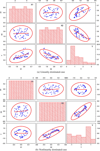
For a given multi-parameter problem $Y=f(X_1,X_2,\dots ,X_n)$, $X\in \mathrm{\Omega }$, if the contribution of an individual parameter $X_i$ is small, the change of $X_i$ will not bring much variation to the objective values Y. Thus $X_i$ and Y should be statistically uncorrelated, or the absolute value of the correlation coefficient will be very small. Based on this fact, we have suggested using a pairwise correlation graph to study multi-parameter problems, in which the data are projected onto a 2-D plane pairwise, and then the correlation coefficient between each parameter and the objective is determined based on data distribution on the 2-D plane. For example, consider a scalar valued problem with two parameters. Both of the parameters $X_1$ and $X_2$ could affect the value of objective Y. One needs to find the RCR of each parameter to the objective value. Suppose a set of 50 samples $\{(x_1^{(i)},x_2^{(i)},y^{(i)}),i=1,2,\dots ,50\}$ has been obtained. To get the pairwise correlation graph, the 50 points are projected onto planes $X_1-X_2$, $X_1-Y$ and $X_2-Y$, respectively, as shown in Figure 1. It is obvious that $X_1$ and $X_2$ are uncorrelated since their correlation ellipses are close to a circle. $X_1$ and Y are positively correlated, while $X_2$ and Y are inversely correlated since their correlation ellipses are both flat and the slopes of ellipse’s semi-major axes are positive and negative, respectively. In fact, the exact relationship between the three variables is $Y=X_1/X_2$, where $(X_1,X_2)\in {[1,5]}^2$ in this case.

Figure 1. An example of pairwise correlation graph.

In general, the proposed pairwise correlation graph can help to identify the qualitative impact of each parameter on the objective value, and can even give a good quantitative value to show the degree of its impact, provided that all of the other parameters have little impact. However, when the parameter and objective have a strong nonlinear relationship, the pair wise correlation graph cannot give helpful information. This can be illustrated by the following example. Suppose we have a set of 50 sample points randomly drawn from the nonlinear function $Y=\left(5\ast X_2+0.2\ast X_1^2\right)/\left(3+{X_1}^2+{X_2}^2\right)$ in the domain $(X_1,X_2)\in {[-5,5]}^2$, and we try to detect the impact of each parameter $X_i(i=1,2)$ on the objective Y. The pairwise correlation graph is presented in Figure 1. It can be seen that the correlation ellipse of $X_1$ and Y is almost round, which means $X_1$ and Y are uncorrelated. This is not what we expect because $X_1$ and Y are actually correlated in the sense of nonlinear correlation. In other words, the pairwise correlation graph has failed to detect the desired correlation in this example.

Another drawback of the pairwise correlation graph is that it might give a misleading result. In fact, in many practical applications, the sample points could not be sampled evenly due to the limitations of experimental conditions. As a result, although the correlation ellipse looks very flat, the parameter and objective are not actually correlated.

Thus, for nonlinear problems with multiple parameters, we need some new concepts to quantitatively measure the relative contribution of each parameter to the objective.

3. Concept of RCR

3.1. Quick view of relevant concepts

As early as 1895, Pearson proposed a concept of correlation coefficient (Pearson, 1895). Although this concept is defined in 2-D space, it is still used to analyze multi-parameter problems in many practical applications. Pearson’s correlation coefficient is strongly dependent on linearity. So Spearman (1904/2010) introduced a rank concept for correlation, which enables it to be capable of analyzing problems with monotone decreasing (or increasing) relationships. Thereafter, Kendall (1938) introduced another new concept of concordant and discordant, and made a further extension of correlation. Both Spearman and Kendall’s correlation coefficients can depict part of the nonlinear relationship provided that there exists some partial ordering relations between the parameter and the objective. However, all of the above three correlation coefficients might fail to get the right correlation in general nonlinear cases. To address this problem, Wang, Shen, and Zhang (2005) proposed a nonlinear correlation measure, nonlinear correlation information entropy (NCIE), defined as $\text{NCC}(X;Y)=H^r(X)+H^r(Y)-H^r(X,Y)$, where $H^r(X,Y)$ is the revised joint entropy of the two variables X and Y. Zheng, Shi, and Zhang (2012) proposed a new concept, generalized measure of correlation (GMC) as follows.$$\{\text{GMC}(Y|X),\text{GMC}(X|Y)\}=\left\{1-\frac{E({\{Y-E(Y|X)\}}^2)}{\text{var}(Y)},1-\frac{E({\{X-E(X|Y)\}}^2)}{\text{var}(X)}\right\}$$

Both NCIE and GMC can handle nonlinear correlation problems properly. However, essentially, both of the metrics are still defined in a 2-D space and using the two metrics it is difficult to analyze data with multiple parameters for their relative contributions/queryPlease check the edits made in the sentence “However, essentially ... relative contributions.” And correct if necessary.. This motivates us to make a further extension of these concepts to n-D space.

3.2. Definition of relative ratio of contribution

Existing correlation coefficients are all defined in a 2-D space. To handle multi-parameter problems, one has to resort to dimensionality reduction, and project the data onto a 2-D plane pair by pair, as illustrated in Section 2. This could give misleading results, as discussed in Sections 2 and 3.1.

In our opinion, during the above projection process, the information contained in the data is over-compressed, and useful information might be lost. In our new concept, we try to define a less compressed projection process, so as to keep the valuable information as much as possible. That is, among the several parameters $X_1,X_2,\dots ,X_n$, to determine the contribution of parameter $X_i$, the sampled data are projected onto its complement space $(X_1,X_2,\dots ,X_{i-1},X_{i+1},\dots ,X_n)-Y$. The projection is mapped from (n + 1)-D space to n-D space $P:R^{n+1}\mapsto R^n$. Only one dimension is reduced during the projection. Thus, more information could be retained.

The parameter $X_i$ will be absent after the projection process. It is obvious that the projected points will become more divergent if $X_i$ has much contribution to the objective Y. Otherwise, the divergence will be little, and the projected points will converge to a curve (in 2-D), surface (in 3-D), or hypersurface (in k-D, $k\le n$). To quantitatively measure its degree of convergence , we suggest using a surrogate model as the reference object. 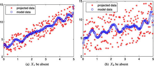The surrogate model $m_i(X_1,X_2,\dots ,X_{i-1},X_{i+1},\dots ,X_n)$ is a data-driven model, determined by the projected points. The more divergent they are, the further they will deviate from the model. To illustrate the relationship between the relative contribution of a parameter and the divergence of projected data, we take a simple intuitive example as follows. Suppose we have a set of 200 sample points uniformly drawn from the rectangular region ${[0,5]}^2$, and the objective function has an explicit expression $Y_1=X_1+2X_2$, then we can get an illustrative result of each parameter’s relative contribution to the 200 points $(x_1^{(k)},x_2^{(k)},y^{(k)})$, $k=1,2,\dots ,200$ as follows. First, project these points onto plane $X_2-Y_1$ and $X_1-Y_1$ respectively, and then draw their data-driven models (see Figure 2(a) and (b)). It can be seen that the projected points are much more divergent when $X_2$ is absent, which means the parameter $X_2$ has more contribution to the objective Y than the parameter $X_1$. Of course, the actual RCR is known in this example, i.e. $X_2$ has double contribution than $X_1$. This example is used only for demonstration. In practical applications, the RCR is not so easy to observe in general.

Figure 2. Divergence of projected points and the deviation from the data-driven model.

Figure 3. Divergence of projected points and the deviation from the observation-prediction line.

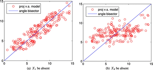
If the problem involves only two parameters, $X_1$ and $X_2$, the divergence of the projected points can be easily shown with a scatter-point plot on a 2-D plane, as shown in Figure 2(a) and (b). Similarly, 3-D scatter-point plot can also be used to show the divergence of the projected points if there are only three influence parameters $X_1$, $X_2$ and $X_3$. However, scatter-point plot cannot help if the problem involves four or more influence parameters, which is usual in practical applications. So we suggest using an observation-prediction plot $(Y,m_i(X_1,X_2,\dots ,X_{i-1},X_{i+1},\dots ,X_n))$ to show the divergence of the projected points, where the observation denotes the objective value of samples, and the prediction denotes their predicted value with the data-driven model $m_i$. The more divergent the projected points are, the further they will deviate from the observation-prediction line segment (on the angle bisector of the first and third quadrants). For the above case, its observation-prediction figures are shown in Figure 3(a) and (b).

Based on these facts, the RCR of $X_i$ to its objective function f can be defined as follows.

Definition 1

Suppose the function $Y=f(X_1,X_2,\dots ,X_n)$ is continuous and bounded on the box-constrained domain $\mathrm{\Omega }$, where $f:\mathrm{\Omega }\mapsto R$, $(X_1,X_2,\dots ,X_n)\in \mathrm{\Omega }\subset R^n$. Let the subspace $S_{X_i}=(X_1,X_2,\dots ,X_{i-1},X_{i+1}$, $\dots ,X_n,Y)=R^n$ be the orthogonal complement of $X_i$, the continuous region $P_{f,X_i}\subset S_{X_i}$ be the projection of the hypersuface $Y=f(X_1,X_2,\dots ,X_n)$ onto the subspace $S_{X_i}$, the scalar $V_{f,X_i}$ be the volume (or area in 2-D space) of $P_{f,X_i}$ in its subspace, $i=1,2,\dots ,n$. Then the RCR (RCR) of $X_i$ to its objective function f is defined as $r_{X_i}=\frac{V_{f,X_i}}{{\sum }_{i=1}^n{V}_{f,X_i}}$.

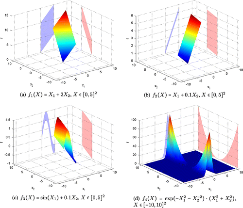
In this definition, the volume/area of the projection reflects the divergence brought by the absence of parameter $X_i$. As a special case, when n = 2, the above definition has a geometric interpretation, which will be illustrated by some simple examples in Figure 4. The first two functions are linear and it is easy to get the volume of projection (the area of the projected parallelogram). From Figure 4(a), one can see that the area of the projection on the complemented subspace of $X_2$ (on the left) is twice that of $X_1$ (on the left). So it is easy to get the RCR $r_{X_1}=1/3$, and $r_{X_2}=2/3$. Similarly, for the example in Figure 4(b), we have $r_{X_1}=1/11$, and $r_{X_2}=10/11$. The RCR is proportional to the product of its absolute coefficient and interval length.

Figure 4. Geometric interpretation of RCR.

As can be seen, the RCR of each parameter is easy to get if the problem is linear. However, it is not so easy to get the volume of projection when the problem is nonlinear (see Figure 4(c) and (d)), and the difficulty will increase as the problem involves more parameters (say, n is above 3). Therefore, special algorithms are needed to calculate RCR. To this end, a surrogate model-based method is proposed in the following section.

4. Numerical computation of RCR

Suppose the objective function has an explicit expression $Y=f(X_1,X_2,\dots ,X_n)$, as examples in Figure 4, the RCR can be approximated by the following steps.

Step 1.	(Random sampling) Randomly generate a sufficient number of sample points $(x_1^{(k)},x_2^{(k)},\dots ,x_n^{(k)})$ within the given domain $\mathrm{\Omega }$, and calculate their corresponding objective values $f^{(k)}$, $k=1,2,\dots ,K$. The sample data forms an (n + 1)-by-K matrix, where each row is determined by a sample point, the first n columns indicate its parameter values, and the last column gives its objective values.
Step 2.	(Subspace projecting) For each influence parameter $X_i$, remove its corresponding column for the (n + 1)-D data to make $X_i$ absent. The projected points lie in space $(X_1,X_2,\dots ,X_{i-1},X_{i+1},\dots ,X_n)-Y$.
Step 3.	(Data-driven modeling) Construct a surrogate model $Y=m_i(X_1,\dots ,X_{i-1},X_{i+1},\dots ,X_n)$ based on the projected points and their corresponding objective values $(x_1^{(k)},\dots ,x_{i-1}^{(k)},x_{i+1}^{(k)},\dots ,x_n^{(k)})$ and $f^{(k)}$.
Step 4.	(Residuals summarizing) Find the total residual $V_i={\sum }_{k=1}^K\left|f^{(k)}-m_i(x_1^{(k)},\dots ,x_{i-1}^{(k)},x_{i+1}^{(k)},\dots ,x_n^{(k)})\right|.$
Step 5.	(Cycling) Repeat step 2 to step 4 until all total residuals $V_i$ are obtained, $i=1,2,\dots ,n$, and let the residual represent the volume of projection $V_{f,X_i}=V_i$ (since they are proportional to each other). Calculate and output the RCRs $r_{X_i}=\frac{V_{f,X_i}}{{\sum }_{i=1}^n{V}_{f,X_i}}$.

In the above steps, the surrogate modeling plays the most important role, in which the approximation models are constructed with a set of sample points. Although increasing the number of samples could help get better models, it will involve much higher computation costs. To enhance the stability and efficiency of the algorithm, the distribution of the samples should be as uniform as possible. Therefore, controlled sampling methods such as Latin hypercube sampling (Beachkofski & Grandhi, 2002) and orthogonal sampling (Steinberg & Lin, 2006) are preferred for sample generation.

After the sample generation and projection, one needs to choose a reliable method for data-driven modeling. There are many model construction methods, including classical linear/nonlinear fitting/interpolation, Kriging regression, radial basis function (RBF) interpolation/regression (Wendland, 2010), and parse matrix evolution (PME) (Luo & Zhang, 2012). For classical fitting/interpolation, the configuration of the model structure does not lead to a good approximation, especially in multidimensional space. RBF interpolation/regression and PME are distinguished for their good performance with fewer requirements on the number of sample points. Kriging regression is famous for its capability of noise-resistance. Note that the distribution of the projected points could be rugged in the subspace. Therefore, an improved version of Kriging regression, DACE (Lophaven, Nielsen, & Søndergaard, 2002), is recommended for the surrogate modeling to ensure its robustness.

For example, consider the problems in Figure 4 with the above method, randomly generate 100 sample points by Latin hypercube sampling, and use DACE for the model construction in the subspace, one can get each parameter’s RCR as follows. $r_{X_1}=0.33$, $r_{X_2}=0.67$ for the first problem; $r_{X_1}=0.09$, $r_{X_2}=0.91$ for the second problem; $r_{X_1}=0.83$, $r_{X_2}=0.17$ for the third problem; And $r_{X_1}=0.57$, $r_{X_2}=0.43$ for the forth problem.

However, in most practical applications, no explicit function is available to describe the relationship between the influence parameters and the objective, and only some test data or simulation results could be obtained. Note that these sample data contain meaningful information that reflects their influence relationship. Therefore, again, we can use DACE to construct a surrogate model to represent the objective function before the first step. Then the RCR could be determined by following the above steps.

Note that DACE needs sufficient number of sample points to construct a surrogate model of high fidelity. This could be quite costly in practical applications. Therefore, in the case of small-sized samples (the amount of data is small relative to the number of influence parameters), we suggest using PME (Luo & Zhang, 2012) or radial basis function interpolation/regression (Wendland, 2010) to construct the surrogate model to approximate the underlying function.

5. A real-world application

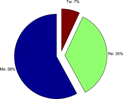
As mentioned in Section 1, for a hypersonic aircraft, several parameters could affect its axial force coefficient $C_A$, including Mach number (Ma), Reynolds (Re) and wall temperature ratio (${\widehat{T}}_w)$. It is of great importance to properly evaluate the relative influence ratio of each parameter for the aircraft design and the behavior control. Suppose we have got sufficient number of sample points for a given aircraft in a certain domain by wind tunnel tests, flight tests and validated CFD simulations, and the surrogate model has been deduced by PME (the surrogate modeling procedure is omitted here):$$C_A=0.029+0.907\left(\frac{1}{M{a}^2}+\frac{1}{R{e}^{1/4}}+\frac{0.260}{{\widehat{T}}_w}\right)$$

where the Mach number $Ma\in [5,8]$, Reynolds $Re\in [3.8\times {10}^5,4.8\times {10}^7]$, and wall temperature $T_w\in [60,250.3]$ K. With the method described in the above section, the RCR of Ma, Re and ${\widehat{T}}_w$ is 58, 35 and 7%, respectively (Figure 5).

Figure 5. The RCR of Ma, Re and Tw to the axial force of an aircraft at hypersonic flight conditions.

6. Conclusion

Motivated by the real-world problem, to measure each parameter’s relative contribution to the aerodynamic-force coefficient of a hypersonic vehicle, a new concept, RCR, has been presented. It considers the relative impact of absence of every parameter by projecting onto its orthogonal complement subspace. Thus, only one dimension is reduced, and more valuable information of the original data is maintained. This makes RCR capable of dealing with multi-parameter problems with linear or non-linear relations. RCR has provided an intuitive way to quantitatively assess different parameters’ relative contribution to the aerodynamic coefficient of hypersonic vehicles, and it can also be used as a scientific metric for other multi-parameter problem analyses without any subjective prejudice.

Based on surrogate modeling, random sampling, subspace projecting, and data-driven modeling, a problem specific algorithm to calculate the RCR is also provided. The proposed algorithm has a good feature of global optimization and has shown its reliability in practice, which brings great convenience in the application of the algorithm.

The concept presented in this paper (RCR) is domain dependent. It is defined on a given domain ($\mathrm{\Omega }$), and the RCR value of a parameter will vary if the range of any parameter has changed. Therefore, this concept is easy to be extended to a local one, or even in the limit sense. These topics will be addressed in our future study.

Additional information

Funding

This research has been supported by Innovation Grant of Chinese Academy of Sciences and the National Natural Science Foundation of China [grant number 90916028].

Notes on contributors

Changtong Luo

The authors are from the group of Shock Wave and Detonation Physics (SWDP), under the supervision of Professor Zonglin Jiang. The research activities are concentrated on hypersonic aerodynamics, especially shock wave and detonation, as well as their applications by theoretical analysis, numerical simulation and physical experiment. The team has set up a large scale shock tunnel (JF–12) with long test duration (100–130 ms), and a hypervelocity shock-expansion tube (JF–16). This paper is motivated by a real-world application of hypersonic aerodynamics, and provides a quantitative metrics to assess the contribution of different parameters to the objective.

References

- Anderson, Jr., J. (2006). Hypersonic and high temperature gas dynamics. Reston, VA: American Institute of Aerodynamics and Astronautics.
- Beachkofski, B., & Grandhi, R. (2002). Improved distributed hypercube sampling ( AIAA Paper Number 2002–1274). Reston, VA: American Institute of Aeronautics and Astronautics.
- Kendall, M. (1938). A new measure of rank correlation. Biometrika, 30, 81–89.
- Lophaven, S. N., Nielsen, H., & Søndergaard, J. (2002). DACE---A Matlab kriging toolbox (pp. 1–26, IMM-REP-2002-12). Kongens Lyngby: Technical University of Denmark.
- Luo, C. T., & Zhang, S.-L. (2012). Parse-matrix evolution for symbolic regression. Engineering Applications of Artificial Intelligence, 25, 1182–1193.
- Pearson, K. (1895). Notes on regression and inheritance in the case of two parents. Proceedings of the Royal Society of London, 58, 240–242.
- Spearman, C. (1904/2010). The proof and measurement of association between two things. The American Journal of Psychology, 15, 72–101; Reprinted by International Journal of Epidemiology, 39, 1137–1150.
- Steinberg, D. M., & Lin, D. K. J. (2006). A construction method for orthogonal Latin hypercube designs. Biometrika, 93, 279–288.
- Wang, Q., Shen, Y., & Zhang, J. (2005). A nonlinear correlation measure for multivariable data set. Physica D: Nonlinear Phenomena, 200, 287–295.
- Wendland, H. (2010). Scattered data approximation. Cambridge: Cambridge University Press.
- Zheng, S., Shi, N.-Z., & Zhang, Z. (2012). Generalized measures of correlation for asymmetry, nonlinearity, and beyond. Journal of the American Statistical Association, 107, 1239–1252.