Nonlinear least squares algorithm for identification of hazards

Abstract

Given observations of selected concentrations one wishes to determine unknown intensities and locations of the sources for a hazard. The concentration of the hazard is governed by a steady-state nonlinear diffusion–advection partial differential equation and the best fit of the data. The discretized version leads to a coupled nonlinear algebraic system and a nonlinear least squares problem. The coefficient matrix is a nonsingular M-matrix and is not symmetric. Iterative methods are compositions of nonnegative least squares and Picard/Newton methods, and a convergence proof is given. The singular values of the associated least squares matrix are important in the convergence proof, the sensitivity to the parameters of the model, and the location of the observation sites.

Keywords:

• advection–diffusion
• impulsive sources
• Schur complement
• nonnegative least squares
• nonlinear
• singular values

AMS subject classifications:

• 35K60
• 65H10
• 93B40
• 93E24

Public Interest Statement

Chemical or biological hazards can move by diffusion or fluid flow. The goal of the research is to make predictions about the location and intensities of the hazards based on the down stream location of observations sites. Mathematical models of the diffusion and flow are used to extrapolate from the observations data sites to unknown upstream locations and intensities of the hazards. The convergence of the iterative process for these extrapolations is studied. The sensitivities of the calculations, because of variations of the model parameters, observation data, and location of the observation sites, are also studied.

1. Introduction

The paper is a continuation of the work in White (2011). The first new result is a convergence proof of the algorithm to approximate a solution to a nonlinear least square problem. A second new result is a sensitivity analysis of the solution as a function of the model parameters, measured data, and observation sites. Here, the singular value decomposition of the least squares matrix plays an important role.

A convergence proof is given for the algorithm to approximate the solution of a coupled nonlinear algebraic system and a nonnegative least squares problem, see lines (9–11) in this paper and in White (2011). These discrete models evolve from the continuous models using the advection–diffusion PDE in Equation (1) (see Pao, 1992). In contrast to the continuous models in Andrle and El Badia (2015), Hamdi (2007), and Mahar and Datta (1997), this analysis focuses on the linear and semilinear algebraic systems. In Hamdi (2007), the steady-state continuous linear model requires observations at all of the down stream portions of the boundary. In Andrle and El Badia (2015), the continuous linear velocity free model where the intensities of the source term are time dependent requires observations at the boundary over a given time interval. In both these papers, the Kohn–Vogelius objective function is used for the symmetric models in the identification problems.

Here and in White (2011) we assume the coefficient matrix associated with the steady-state discretized partial differential equation in Equation (1) is an M-matrix and may not be symmetric, which includes coefficient matrices from upwind finite difference schemes for the advection–diffusion PDE. The least squares matrix C( : , ssites), see Equations (6–8), is an $k\times l$ matrix where $k>l$ and k and l are the number of observation and source sites, respectively. The rank and singular values (see Meyer, 2000, section 5.12), of C( : , ssites) determines whether of not the observation and source sites are located so that the intensities can be accurately computed.

Four examples illustrate these methods. The first two examples in Section 3 are for $n=2$ and $n=3$ unknowns, and they show some of the difficulties associated with the nonlinear problem. Sections 4 and 5 contain the convergence proof. Examples three and four in Section 6 are applications of the 1D and 2D versions of the steady-state advection–diffusion PDE. Sensitivity of the computed solutions due to variation of the model parameters, the data and the relative location of the source and observation sites is illustrated. The connection with the sensitivity and the singular values of the least squares matrix is established.

2. Problem formulation

Consider a hazardous substance with sources from a finite number of locations. The sources are typically located at points in a plane and can be modeled by delta functionals. The hazard is described as concentration or density by a function of space and time, u(x, y, t). This is governed by the advection–diffusion PDE(1) $$\begin{array}{c}\hfill u_t-\mathrm{\nabla }\bullet D\mathrm{\nabla }u+v\bullet \mathrm{\nabla }u+d_{r}u=f(u)+S\end{array}$$(1)

where S is a source term, D is the diffusion, v is the velocity of the medium, $d_r$ is the decay rate, and f(u) is the nonlinear term such as in logistic growth models. The source term will be a finite linear combination of delta functionals(2) $$\begin{array}{c}\hfill S=\sum a_i\mathit{\delta }(x-{\widehat{x}}_i)\end{array}$$(2)

where the coefficients $a_i$ are the intensities and the locations ${\widehat{x}}_i$ are possibly unknown points in the line or plane. The source coefficients should be nonnegative, which is in contrast with impulsive culling where the coefficient of the delta functionals are negative and have the form $-c_{i}u(x_i)$ (see White, 2009).

We will assume the source sites and the observation sites do not intersect. The reason for this is the ability to measure concentrations most likely allows one to measure the intensities at the same site.

Identification problem: Given data for u(osites) at a number of given observation sites, osites,  determine the intensities ($a_i$) and locations (${\widehat{x}}_i$) at source sites, ssites, so that$$\begin{array}{c}\hfill \Vert data-u(osites)\Vert \text{is suitably small}.\end{array}$$

2.1. Linear least squares

Since the governing PDE is to be discretized, we first consider the corresponding linear discrete problem$$\begin{array}{c}\hfill Au=d.\end{array}$$

The coefficient matrix A is derived using finite differences with upwind finite differences on the velocity term. Therefore, we assume A is a nonsingular M-matrix (see Berman & Plemmons, 1994, chapter 6 or Meyer, 2000, section 7.10). The following approach finds the solution in one least squares step. The coefficient matrix is $n\times n$ and nodes are partitioned into three ordered sets, whose order represents a reordering of the nodes:$$\begin{array}{cc}\hfill osites& \text{observe sites}\hfill \\ \hfill ssites& \text{source sites and}\hfill \\ \hfill rsites& \text{remaining sites}.\hfill \end{array}$$

The discrete identification problem is given data data at osites, find d(ssites) such that$$\begin{array}{c}\hfill Au=d\text{such that}u(osites)=data.\end{array}$$

In general, the reordered matrix has the following $2\times 2$ block structure with $other=\left[ssitesrsites\right]$(3) $$\begin{array}{cc}\hfill A& =\left[\begin{array}{cc}a\hfill & e\hfill \\ f\hfill & b\hfill \end{array}\right]\hfill \end{array}$$(3)

where $a=A(osites,osites)$, $e=A(osites,other)$, $f=A(other,osites)$ and $b=A(other,other)$.

Assumptions of this paper:

(1)	A is an M-matrix so that A and a have inverses.
(2)	$\#(osites)=k$, and $\#(ssites)=l<k$ so that $n=k+l+\#(rsites)$.
(3)	$d={\left[0d_1^T\right]}^T$ and the only nonzero terms in $d_1$ are at the nodes in ssites, that is, $d\equiv {\left[0d_1{(ssites)}^{T}0\right]}^T={\left[0z^{T}0\right]}^T$.

Multiply Equation (3) by a block elementary matrix (as in assumptions 1 and 2)(4) $$\begin{array}{cc}& \left[\begin{array}{cc}{I}_k\hfill & 0\hfill \\ -f{a}^{-1}\hfill & I_{n-k}\hfill \end{array}\right]\left[\begin{array}{cc}a\hfill & e\hfill \\ f\hfill & b\hfill \end{array}\right]\left[\begin{array}{c}{u}_0\\ u_1\end{array}\right]=\left[\begin{array}{cc}{I}_k\hfill & 0\hfill \\ -f{a}^{-1}\hfill & I_{n-k}\hfill \end{array}\right]\left[\begin{array}{c}0\\ d_1\end{array}\right]\hfill \end{array}$$(4) (5) $$\begin{array}{cc}& \left[\begin{array}{cc}a\hfill & e\hfill \\ 0\hfill & \widehat{b}\hfill \end{array}\right]\left[\begin{array}{c}{u}_0\\ u_1\end{array}\right]=\left[\begin{array}{c}0\\ d_1\end{array}\right]\hfill \end{array}$$(5)

where $\widehat{b}\equiv b-f{a}^{-1}e$. Solve Equation (5) for $u_1$ and then $u_0=-a^{-1}e{(\widehat{b})}^{-1}{d}_1$. Define(6) $$\begin{array}{c}\hfill d_1\equiv {[d_1{(ssites)}^{T}0]}^T\text{and}C\equiv -a^{-1}e{(\widehat{b})}^{-1}.\end{array}$$(6)

The computed approximations of the observed data are in $u_0$ and the source data are in $z=d_1(ssites)$. This gives a least squares problem for z (7) $$\begin{array}{c}\hfill data=C(:,ssites)z.\end{array}$$(7)

Since a is $k\times k$, e is $k\times (n-k)$, and $\widehat{b}$ is $(n-k)\times (n-k)$, the matrix C is $k\times (n-k)$ and the least squares matrix C( : , ssites) is $k\times l$ where $k>l$. The least squares problem in (7) has a unique solution if the columns of C( : , ssites) are linearly independent ($C(:,ssites)z=0$ implies $z=0)$.

Impose the nonnegative condition on the components of the least squares solution. That is, consider finding $z\ge 0$ such that(8) $$\begin{array}{c}\hfill r{(z)}^{T}r(z)=\underset{y\ge 0}{min}r{(y)}^{T}r(y)\text{where}r(z)\equiv data-C(:,ssites)z\end{array}$$(8)

If the matrix C( : , ssites) has full column rank, then the nonnegative least squares problem (8) has a unique solution (see Bjorck, 1996, section 5.2). The nonnegative least squares solution can be computed using the MATLAB command lsqnonneg.m (see MathWorks Inc., 2015).

2.2. Least squares and nonlinear term

Consider a nonlinear variation of $Au=d$(9) $$\begin{array}{c}\hfill Au=d(z)+\widehat{d}(u)\end{array}$$(9)

where $d(z)={\left[0z^{T}0\right]}^T$ (as in assumption 3) and $\widehat{d}(u)=[{\widehat{d}}_i(u_i)]$.

Use the reordering in (3) and repeat the block elementary matrix transformation in (4) and (5) applied to the above. Using the notation $\widehat{d}(u)={[{\widehat{d}}_0{(u)}^T{\widehat{d}}_1{(u)}^T]}^T$ one gets$$\begin{array}{cc}\hfill \left[\begin{array}{cc}a\hfill & e\hfill \\ 0\hfill & \widehat{b}\hfill \end{array}\right]\left[\begin{array}{c}{u}_0\\ u_1\end{array}\right]& =\left[\begin{array}{cc}{I}_k\hfill & 0\hfill \\ -f{a}^{-1}\hfill & I_{n-k}\hfill \end{array}\right]\left(\left[\begin{array}{c}0\\ d_1\end{array}\right]+\left[\begin{array}{c}{\widehat{d}}_0(u)\\ {\widehat{d}}_1(u)\end{array}\right]\right)\hfill \\ & =\left[\begin{array}{c}0\\ d_1\end{array}\right]+\left[\begin{array}{c}{\widehat{d}}_0(u)\hfill \\ -f{a}^{-1}{\widehat{d}}_0(u)+{\widehat{d}}_1(u)\hfill \end{array}\right].\hfill \end{array}$$

Solve for $u_1$ and then for $u_0$$$\begin{array}{cc}\hfill u_0& =a^{-1}{\widehat{d}}_0(u)-a^{-1}e{(\widehat{b})}^{-1}\left(d_1+(-f{a}^{-1}{\widehat{d}}_0(u)+{\widehat{d}}_1(u))\right)\hfill \\ \hfill & =g(u)+C{d}_1\hfill \end{array}$$

where $C\equiv -a^{-1}e{(\widehat{b})}^{-1}$ and $g(u)\equiv a^{-1}{\widehat{d}}_0(u)+C(-f{a}^{-1}{\widehat{d}}_0(u)+{\widehat{d}}_1(u))$.

This leads to a nonlinear least squares problem for nonnegative z (10) $$\begin{array}{c}\hfill data-g(u)=C(:,ssites)z.\end{array}$$(10)

The solution of the nonnegative least squares problem is input to the nonzero components in d, that is, $d(ssites)=z$. The coupled problem from (9) and (10) is to find $z\ge 0$ and u so that(11) $$\begin{array}{c}\hfill data-g(u)=C(:,ssites)z\text{and}Au=d(z)+\widehat{d}(u).\end{array}$$(11)

3. Two algorithms for the coupled problem

If the nonnegative least squares problem has a unique solution $z=H(u)$ given a suitable u, then we can write (11) as$$\begin{array}{c}\hfill Au=d(H(u))+\widehat{d}(u),\end{array}$$

or as a fixed point$$\begin{array}{c}\hfill u=A^{-1}(d(H(u))+\widehat{d}(u))\equiv G(u).\end{array}$$

The following algorithm is a composition of nonnegative least squares and a Picard update to form one iteration step. Using additional assumptions we will show this is contractive and illustrate linear convergence. Example 3.2 is a simple implementation with $n=3$, and in Section 6 Example 6.1 uses the 1D steady-state version of the model in (1) and Example 6.2 uses the 2D steady-state model in (1).

Algorithm 1. NLS-Picard Method for (11)       choose nonnegative $u^0$       for $m=0$, mmax             solve the nonnegative least squares problem                   $data-g(u^m)=C(:,ssites)z^{m+1}$             solve the linear problem                   $A{u}^{m+1}=d(z^{m+1})+\widehat{d}(u^m)$             test for convergence       end for-loop

The following algorithm uses a combination of nonnegative least squares and Newton like updates. Define F(z, u) and $F_u(z,u)$ as$$\begin{array}{c}\hfill F(z,u)\equiv Au-d(z)-\widehat{d}(u)\text{and}{F}_u(z,u)\equiv A-0-{\widehat{d}}_u(u)\end{array}$$

where ${\widehat{d}}_u(u)\equiv [{({\tilde{d}}_i)}^{\prime }(u_i)]$ is the diagonal matrix with components ${({\tilde{d}}_i)}^{\prime }(u_i)$.

The matrix $F_u(z,u)$ is not the full derivative matrix of F(z, u) because it ignores the dependence of z on u. Choose $\mathit{\lambda }>0$ so that $F_u+\mathit{\lambda }I$ has an inverse.

Algorithm 2. NLS-Newton Method for (11)       choose nonnegative $u^0$and $\mathit{\lambda }>0$       for $m=0$, mmax             solve the nonnegative least squares problem                   $data-g(u^m)=C(:,ssites)z^{m+1}$             solve the linear problem                   $A{u}^{m+1/2}=d(z^{m+1})+\widehat{d}(u^m)$             compute $F(z^{m+1},u^{m+1/2})\equiv A{u}^{m+1/2}-d(z^{m+1})-\widehat{d}(u^{m+1/2})$                   $=\widehat{d}(u^m)-\widehat{d}(u^{m+1/2})$             compute $F_u(z^{m+1},u^{m+1/2})\equiv A-0-{\widehat{d}}_u(u^{m+1/2})$             solve the linear problem                   $(F_u(z^{m+1},u^{m+1/2})+\mathit{\lambda }I)\mathrm{\Delta }u=F(z^{m+1},u^{m+1/2})$             $u^{m+1}=u^{m+1/2}-\mathrm{\Delta }u$             test for convergence       end for-loop

Variations of the NLS-Newton algorithm include using over relaxation, $\mathit{\omega }$, at the first linear solve and using damping, $\mathit{\alpha }$, on the second linear solve in the Newton update:$$\begin{array}{cc}\hfill u^{m+1/2}& =(1-\mathit{\omega })u^m+\mathit{\omega }{u}^{m+1/2}\text{and}\hfill \\ \hfill u^{m+1}& =u^{m+1/2}-\mathit{\alpha }\mathrm{\Delta }u.\hfill \end{array}$$

Appropriate choices of $w,\mathit{\alpha }$ and $\mathit{\lambda }$ can accelerate convergence.

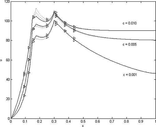
The calculations recorded in Table 4 and Figure 4 in White (2011), illustrate the NLS-Newton algorithm for the 1D steady-state problem with logistic growth term $\widehat{d}(u)=f(u)=c(100-u)u$ and variable growth rate c. The larger the c parameter resulted in larger concentrations. The intensities at the three source sites were identified. However, the number of iterations of the NLS-Newton algorithm increased as the c parameter increased. The algorithm did start to fail for c larger than 0.0100.

The lack of convergence is either because the associated fixed point problem does not have a contractive mapping or because the solutions become negative. The following example with $n=2$, nonzero source term and nonsymmetric A illustrates the difficulty of solving a semilinear algebraic problem where the solution is required to be positive.

Example 3.1

Let $n=2$ and use $f_i(u_i)=c(100-u_i)u_i$. Equation (9) has the form$$\begin{array}{c}\hfill \left[\begin{array}{cc}1& 0\\ -\mathit{\epsilon }& 1\end{array}\right]\left[\begin{array}{c}{u}_0\\ u_1\end{array}\right]=\left[\begin{array}{c}0\\ z\end{array}\right]+\left[\begin{array}{c}{f}_0(u_0)\\ f_1(u_1)\end{array}\right].\end{array}$$

The first equation is $u_0=c(100-u_0)u_0$ whose solution is either $u_0=0$ or $u_0=100-1/c>0$. Put the nonzero solution into the second equation $-\mathit{\epsilon }(100-1/c)+u_1=z+c(100-u_1)u_1$ and solve for $u_1$. If $\mathit{\epsilon }(100-1/c)+z>0$, then the second equation is $u_1=c(100-u_1)u_1+\mathit{\epsilon }(100-1/c)+z$ and will have a positive solution.

The next example with $n=3$, given data at the first and second nodes and a source term at the third node illustrates the coupled problem in (11). This simple example can be solved both by-hand calculations and the NLS-Picard algorithm, and more details are given in Appendix 1.

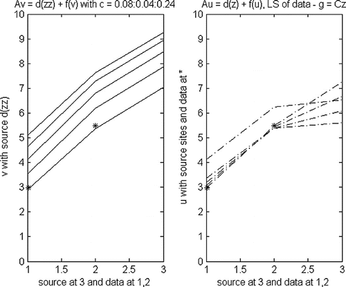
Example 3.2

Let the data be given at the first and second nodes$$\begin{array}{c}\hfill data=\left[\begin{array}{c}2.9711\\ 5.4971\end{array}\right].\end{array}$$

Let the matrix A and nonlinear terms be given by system$$\begin{array}{c}\hfill \left[\begin{array}{ccc}3& 0& -1\\ 0& 3& -2\\ -2& -2& 4\end{array}\right]\left[\begin{array}{c}{u}_1\\ u_2\\ u_3\end{array}\right]=\left[\begin{array}{c}0\\ 0\\ z\end{array}\right]+\left[\begin{array}{c}c{u}_1(10-u_1)\\ c{u}_2(10-u_2)\\ c{u}_3(10-u_3)\end{array}\right].\end{array}$$

The submatrices of A are$$\begin{array}{c}\hfill a=\left[\begin{array}{cc}3& 0\\ 0& 3\end{array}\right],e=\left[\begin{array}{c}-1\\ -2\end{array}\right],f=\left[\begin{array}{cc}-2& -2\end{array}\right]\text{and}b=[4].\end{array}$$

Then one easily computes$$\begin{array}{c}\hfill \widehat{b}=b-f{a}^{-1}e=\left[2\right]\text{and}C=-a^{-1}e{\widehat{b}}^{-1}=(1/6)\left[\begin{array}{c}1\\ 2\end{array}\right].\end{array}$$

The g(u) in the nonlinear least square Equation (11) is$$\begin{array}{c}\hfill g(u)=c\left[\begin{array}{c}(4/9)u_1(10-u_1)+(1/6)u_3(10-u_3)+(1/9)u_2(10-u_2)\\ (5/9)u_2(10-u_2)+(2/6)u_3(10-u_3)+(2/9)u_1(10-u_1)\end{array}\right].\end{array}$$

The calculation with the NLS-Picard algorithm for this example with $n=3$ in White (2015, testlsnonlc.m) confirms both the exact solution for $c=8/100=0.0800$ and convergence for $c<0.1667$, which are given in Appendix 1. The number of iterations needed for convergence increases as c increases, and convergence fails for $c=0.3000$. Both the exact and NLS-Picard calculations show $z>0$ for $c\le 0.1975$ and $z=0$ for $c\ge 0.1976$. The outputs for five values of $c=0.08:0.04:0.24$ are given in Figure 1. The left graphs indicate the five solutions of (10) for fixed $z=zz=10$ and increasing c. The two “*” are the given data, which are from the solution of (10) with $c=0.0800$ and 5% error. The right graphs are the converged solutions of (11) for $c=0.08:0.04:0.20$.

4. Nonnegative least squares problem

The nonnegative least squares problem in (10) for $z\ge 0$ has several forms$$\begin{array}{c}\hfill R{(z)}^{T}R(z)=\underset{y\ge 0}{min}R{(y)}^{T}R(y)\text{where}R(z)\equiv data-g(u)-C(:,ssites)z.\end{array}$$

This may be written as(12) $$\begin{array}{c}\hfill R{(z)}^{T}R(z)={(data-g(u))}^T(data-g(u))-2J(z)\end{array}$$(12)

where$$\begin{array}{c}\hfill J(z)\equiv \frac{1}{2}{z}^{T}C{(:,ssites)}^{T}C(:,ssites)z-z^{T}C{(:,ssites)}^T(data-g(u)).\end{array}$$

Figure 1. NLS-Picard algorithm for n = 3.

If C( : , ssites) has full column rank, then the matrix $C{(:,ssites)}^{T}C(:,ssites)$ is symmetric positive definite (SPD). J(z) is the quadratic functional associated with the linear system (normal equations)$$\begin{array}{c}\hfill 0=r(z)\equiv C{(:,ssites)}^T(data-g(u))-C{(:,ssites)}^{T}C(:,ssites)z\end{array}$$

When the nonnegative condition is imposed on $z\ge 0$ and the matrix is SPD, then the following are equivalent (see Cryer, 1971):$$\begin{array}{cc}& J(z)=\underset{y\ge 0}{min}J(y)\text{(minimum quadratic functional)},\hfill \\ \hfill & 0\ge r{(z)}^T(y-z)\text{for all}y\ge 0\text{(variational inequality) and}\hfill \\ \hfill & 0=r{(z)}^{T}z\text{and}0\ge r(z)\text{(linear complementarity problem).}\hfill \end{array}$$

Any solution of a variational inequality is unique and depends continuously on the right-hand side. The next theorem is a special case of this.

Theorem 4.1

Consider the nonnegative least squares problem in (10). If C( : , ssites) has full column rank, then there is only one nonnegative solution for each u. Let $z=H(u)$ be the solution for each u in S where S is a bounded set of nonnegative n-vectors. Moreover, if $\Vert \widehat{d}(u)-\widehat{d}(v)\Vert \le \widehat{K}\Vert u-v\Vert$, then there is a constant $C_1$ such that$$\begin{array}{c}\hfill \Vert C(:,ssites)(H(u)-H(v))\Vert \le C_1\Vert u-v\Vert \end{array}$$

Proof

Let z and w be solutions of (10). The variational inequalities for z with $y=w$, and for w with $y=z$ are$$\begin{array}{c}\hfill 0\ge r{(z)}^T(w-z)\text{and}0\ge r{(w)}^T(z-w).\end{array}$$

Add these to get a contradiction for the case $z-w$ is not a zero vector$$\begin{array}{c}\hfill 0\ge {(z-w)}^{T}C{(:,ssites)}^{T}C(:,ssites)(z-w)>0.\end{array}$$

In order to show the continuity, use the above with $z=H(u)$ and $w=H(v):$$$\begin{array}{cc}\hfill 0& \ge {[C{(:,ssites)}^T(data-g(u))-C{(:,ssites)}^{T}C(:,ssites)H(u)]}^T(H(v)-H(u))\hfill \\ \hfill 0& \ge {[C{(:,ssites)}^T(data-g(v))-C{(:,ssites)}^{T}C(:,ssites)H(v)]}^T(H(u)-H(v)).\hfill \end{array}$$

Add these to obtain for $B\equiv C{(:,ssites)}^{T}C(:,ssites)$$$\begin{array}{c}\hfill {(H(v)-Hu))}^{T}B(H(v)-H(u))\le -{(g(v)-g(u))}^{T}C(:,ssites)(H(v)-H(u)).\end{array}$$

Use the Cauchy inequality$$\begin{array}{c}\hfill {\Vert C(:,ssites)(H(v)-H(u))\Vert }^2\le \Vert g(v)-g(u)\Vert \Vert C(:,ssites)(H(v)-H(u))\Vert .\end{array}$$

By the definition of g and the assumption on d we have for some $C_1$$$\begin{array}{c}\hfill \Vert C(:,ssites)(H(v)-H(u))\Vert \le C_1\Vert v-u\Vert .\end{array}$$$\square$

The solution of the variational problem for fixed u has the form $z=$H(u). The assumption that C( : , ssites) has full column rank implies there is a positive constant $c_0$ such that $c_0^2{w}^{T}w\le w^{T}C{(:,ssites)}^{T}C(:,ssites)w$. This and the above theorem give the following(13) $$\begin{array}{c}\hfill c_0\Vert H(v)-H(u)\Vert \le \Vert C(:,ssites)(H(v)-H(u))\Vert \le C_1\Vert v-u\Vert .\end{array}$$(13)

Although in Example 3.2 with $n=3$ one can estimate $c_0$ and $C_1$, generally these constants are not easily approximated. However, $c_0$ can be estimated by the smallest singular value of the least squares matrix.

5. Convergence proof of the NLS-Picard algorithm

Let the assumptions in the previous theorem hold so that (12) is true for all $u,v\in S$. The mapping $G(u)\equiv A^{-1}(d(H(u))+\widehat{d}(u))$ may not give $G(u)\in S!$ This appears to be dependent on the particular problem and properties of $\widehat{d}(u)$. If the bound is chosen so that $\widehat{d}(u)$ is also nonnegative, then assumption (1) implies $A^{-1}\ge 0$ and hence $G(u)\ge 0$. The least squares condition requires the solution to be “close” to the given data at the osites, which suggests the G(u) should remain bounded. The following theorem gives general conditions on the problem.

Theorem 5.1

Let the assumptions of Theorem 4.1 hold for $u,v\in S$. Assume there is a solution to the coupled problem (11), $u^{\ast }\in S$. Let $c_0$ and $C_1$ be from (12). If$$\begin{array}{c}\hfill \widehat{r}\equiv \Vert A^{-1}\Vert (C_1/c_0+\widehat{K})<1,\end{array}$$

then the NLS-Picard algorithm will converge to this solution of (11).

Proof

Let $u^{\ast }=G(u^{\ast })$ and $u^{m+1}=G(u^m)$.$$\begin{array}{cc}\hfill ∥u^{\ast }-u^{m+1}∥& =\Vert G(u^{\ast })-G(u^m)\Vert \hfill \\ \hfill & =∥A^{-1}(d(H(u^{\ast })-d(H(u^m))+A^{-1}(\widehat{d}(u^{\ast })-\widehat{d}(u^m))∥\hfill \\ \hfill & \le ∥A^{-1}\Vert (C_1/c_0)\Vert u^{\ast }-u^m\Vert +\Vert A^{-1}\Vert \widehat{K}\Vert u^{\ast }-u^m∥\hfill \\ \hfill & =∥A^{-1}\Vert (C_1/c_0+\widehat{K})\Vert u^{\ast }-u^m∥\hfill \\ \hfill & =\widehat{r}\Vert u^{\ast }-u^m\Vert \hfill \\ \hfill & ⋮\hfill \\ \hfill & \le {\widehat{r}}^{m+1}\Vert u^{\ast }-u^0\Vert .\hfill \end{array}$$

Since $\widehat{r}<1$, this implies convergence $\square$

6. Applications and sensitivity analysis

Both the NLS-Picard and NLS-Newton methods converge linearly, that is, the errors at the next iteration are bounded by a contractive constant, $\widehat{r}<1$, times the error from the current iteration. However, the contractive constant for the NLS-Newton algorithm is significantly smaller than the contractive constant for the NLS-Picard algorithm, and this results in fewer iterations steps for the NLS-Newton algorithm. The calculations in the next two examples can be done by either algorithm. The relevance of the singular values of the least squares matrix to the sensitivity of the calculations with variations in the data and the source and observation sites is demonstrated.

Figure 2. NLS-Newton algorithm with variable c.

Example 6.1

Consider the steady-state 1D model in (1). The following calculations were done by the MATLAB code in White (2015, poll1dlsnonla2.m) and with seven observation sites, three source sites, and $n=160$. The differential Equation (1) was discretized by the upwind finite difference approximations, and the sources terms were the intensities times the approximation of the delta functionals$$\begin{array}{c}\hfill d(ssites)={[a_1{a}_2{a}_3]}^T/dx\end{array}$$

where initially $d\equiv zeros(n,1)$. In order to check the accuracy of the finite difference model, calculations were done with $n=160,320$ and 480, which gave similar results as reported below for $n=160$. The condition number (ratio of the largest and smallest singular values) of the least squares matrix controls the relative errors in the computed least squares problem. The condition numbers for the $n=160,320$, and 480 are about the same at 17.0170, 16.5666, and 16.4146, respectively.

For $c=0.010$ the NLS-Picard algorithm did not converge, but the NLS-Newton algorithm converged in 92 steps. The solid lines in Figure 2 are with no random error in the data, and the dotted lines are from data with 5% random error. For $c=0.005$ the NLS-Picard algorithm converged in 100 steps with $\widehat{r}\approx .83$, and the NLS-Newton algorithm converged in 19 steps with $\widehat{r}\approx .41$. If w is changed from 1.0 to 1.1, then the NLS-Newton algorithm converges in 16 steps with $\widehat{r}\approx .28$. As c decreases, the iterations required for convergence and $\widehat{r}$ decrease.

The dotted lines indicate some uncertainty in the numerical solutions, which can be a function of the physical parameters and the location of the observation sites relative to the source sites. If there is no error in the data, the intensities of the sources are in the vector$$\begin{array}{c}\hfill z=\left[\begin{array}{ccc}4.0000& 1.0000& 2.0000\end{array}\right].\end{array}$$

Use 100 computations with the $c=0.001$ and 5% random errors. The means and standard deviations of the computed intensities at the three source sites are$$\begin{array}{cc}\hfill mean(z)& =\left[\begin{array}{ccc}4.0357& 0.9437& 2.0187\end{array}\right]\text{and}\hfill \\ \hfill std(z)& =\left[\begin{array}{ccc}0.2570& 0.3631& 0.1375\end{array}\right].\hfill \end{array}$$

The standard deviation of the intensities at the center source in Figure 2 is large relative to its mean value. The large computed least squares errors are a result of some relatively small singular values in the singular value decomposition of the least squares matrix$$\begin{array}{c}\hfill C(:,ssites)=U\mathrm{\Sigma }{V}^T\end{array}$$

where the singular values ${\mathit{\sigma }}_i$ are the diagonal components of $\mathrm{\Sigma }$; U is $7\times 7$, $\mathrm{\Sigma }$ is $7\times 3$ and V is $3\times 3$.

In this example, the third singular value is small$$\begin{array}{c}\hfill \mathit{\sigma }=\left[\begin{array}{ccc}0.2882& 0.0916& 0.0169\end{array}\right].\end{array}$$

The least square solution of (10) is given by the pseudo inverse of the least squares matrix times $data-g(u)\equiv \widehat{d}$$$\begin{array}{c}\hfill V{\mathrm{\Sigma }}^{†}{U}^T\widehat{d}=v_1{u}_1^T\widehat{d}/{\mathit{\sigma }}_1+v_2{u}_2^T\widehat{d}/{\mathit{\sigma }}_2+v_3{u}_3^T\widehat{d}/{\mathit{\sigma }}_3.\end{array}$$

Because ${\mathit{\sigma }}_3$ is relatively small, any errors in $\widehat{d}$ will be amplified as well as the components of$$\begin{array}{c}\hfill v_3={\left[\begin{array}{ccc}0.5778& -0.7882& 0.2121\end{array}\right]}^T.\end{array}$$

This suggests the second component, the center source, of least squares solution will have significant errors. The errors can be decreased if the percentage random error is smaller or by alternative location of the observation sites. In the 1D model this is not too difficult to remedy. However, in the 2D model this is more challenging.

Example 6.2

Consider the steady-state 2D model in (1) with boundary conditions equal to zero up stream and zero normal derivative down stream. The calculations in Figure 3 were done by the MATLAB code in White (2015, testlsnonlf2da3.m) using NLS-Picard and with four variable observation sites and three fixed source sites. The three fixed sources are to the left near $x=0$, and the four observation sites are indicated by the symbol “*” above the site. The intensities times the approximation of the delta functionals is$$\begin{array}{c}\hfill d(ssites)={[a_1{a}_2{a}_3]}^T/(dx\ast dy)\end{array}$$

where initially $d\equiv zeros(nn,1)$ and $nn=(nx+1)\ast (ny+1)$. If there is no random error in the data, then the computed source will be$$\begin{array}{c}\hfill \left[\begin{array}{ccc}8.0000& 16.0000& 4.0000\end{array}\right].\end{array}$$

The numerical experiments involve varying the location of the observation site at (x, 16) where $x=L-\mathrm{\Delta }L$ and varying the y-component of the velocity, vely. The velocity term in (1) is $(velx,vely)=(1.00,0.10)$. The base calculation in Figure 3 uses $\mathrm{\Delta }L=30$ and $vely=0.10$ along with 5% random error in the data and $c=0.0004$ growth coefficient in the nonlinear term. The singular values of the least squares matrix and the mean and standard deviations of the intensities of the three computed sources are recorded for 100 computations.

$\mathrm{\Delta }L=30$ and $vely=0.10:$$$\begin{array}{cc}& \mathit{\sigma }=\left[\begin{array}{ccc}0.0472& 0.0300& 0.0046\end{array}\right]\hfill \\ \hfill & mean(z)=\left[\begin{array}{ccc}7.9947& 16.0341& 4.0040\end{array}\right]\text{and}\hfill \\ \hfill & std(z)=\left[\begin{array}{ccc}0.2523& 0.4966& 0.1451\end{array}\right].\hfill \end{array}$$

Changing the y-component of the velocity can cause the concentration to be moved away from the observation sites and cause more uncertainty in the calculations, which is indicated by larger standard deviations and smaller singular values of the least squares matrix. Change $vely=0.10$ to $vely=0.15$ and $vely=0.05$.

$\mathrm{\Delta }L=30$ and $vely=0.15:$$$\begin{array}{cc}& \mathit{\sigma }=\left[\begin{array}{ccc}0.0424& 0.0302& 0.0002\end{array}\right]\hfill \\ \hfill & mean(z)=\left[\begin{array}{ccc}7.9562& 16.034& 23.6939\end{array}\right]\text{and}\hfill \\ \hfill & std(z)=\left[\begin{array}{ccc}0.2399& 0.5479& 30.7650\end{array}\right].\hfill \end{array}$$

Here, the third singular value has significantly decreased and can cause failure of the NLS-Picard algorithm or increased computation errors because of the variation in the data.

$\mathrm{\Delta }L=30$ and $vely=0.05:$$$\begin{array}{cc}& \mathit{\sigma }=\left[\begin{array}{ccc}0.0853& 0.0004& 0.0001\end{array}\right]\hfill \\ \hfill & mean(z)=\left[\begin{array}{ccc}7.7883& 16.6030& 3.9778\end{array}\right]\text{and}\hfill \\ \hfill & std(z)=\left[\begin{array}{ccc}0.5744& 2.0884& 0.1167\end{array}\right].\hfill \end{array}$$

In this case the second and third singular values of the least squares matrix decreased, and the standard deviation of the second source increased.

Changing the location of the third observation site can also cause more uncertainty in the calculations, which is indicated by larger standard deviations and smaller singular values of the least squares matrix. Change $\mathrm{\Delta }L=30$ to $\mathrm{\Delta }L=20$ and $\mathrm{\Delta }L=10$ and keep $vely=0.10$.

$\mathrm{\Delta }L=20$ and $vely=0.10:$$$\begin{array}{cc}& \mathit{\sigma }=\left[\begin{array}{ccc}0.0472& 0.0300& 0.0005\end{array}\right]\hfill \\ \hfill & mean(z)=\left[\begin{array}{ccc}8.0012& 16.0350& 4.5229\end{array}\right]\text{and}\hfill \\ \hfill & std(z)=\left[\begin{array}{ccc}0.2350& 0.5321& 4.5265\end{array}\right].\hfill \end{array}$$

Here, the third singular value has significantly decreased and can cause failure of the NLS-Picard algorithm or increased computation errors because of the variation in the data. The standard deviation of the third source has significantly increased.

$\mathrm{\Delta }L=10$ and $vely=0.10:$$$\begin{array}{cc}& \mathit{\sigma }=\left[\begin{array}{ccc}0.0472& 0.0320& 0.0000396\end{array}\right]\hfill \\ \hfill & mean(z)=\left[\begin{array}{ccc}8.0005& 15.9137& 238.9531\end{array}\right]\text{and}\hfill \\ \hfill & std(z)=\left[\begin{array}{ccc}0.2379& 0.5007& 396.3124\end{array}\right].\hfill \end{array}$$

In this case the third singular values of the least squares matrix have dramatically decreased, and the standard deviation of the third source is very large relative to the mean.

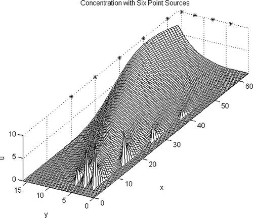
The calculation in Figure 4 has six source sites (near the axes) and nine observation sites (down stream and below the “*”) (White, 2015, testlsnonlf2da6.m) uses NLS-Picard. Here the vely is larger with velocity the equal to (1.00, 0.30), and the random error in the data is smaller and equal to 1%:$$\begin{array}{cc}& \mathit{\sigma }=\left[\begin{array}{cccccc}0.0782& 0.0612& 0.0459& 0.0304& 0.0178& 0.0047\end{array}\right]\hfill \\ \hfill & mean(z)=\left[\begin{array}{cccccc}23.9404& 16.0215& 8.0135& 3.9869& 16.1539& 7.9334\end{array}\right]\text{and}\hfill \\ \hfill & std(z)=\left[\begin{array}{cccccc}0.8512& 0.4408& 0.2064& 0.0549& 0.9046& 0.2879\end{array}\right].\hfill \end{array}$$

The source closest to the origin is the most difficult to identify; with one percent error in the data the standard deviation is 0.8512 and with five percent error this goes up to 4.2348. This happens despite the relatively close distribution of the singular values from 0.0782 to 0.0047 for a condition number equal to 16.7658.

7. Summary

In order to determine locations and intensities of the source sites from data at the observation sites, there must more observations sites than source sites and the observation sites must be more chosen so that the least squares matrix C( : , ssites) has full column rank. Furthermore, the singular values in the singular value decomposition of the least squares matrix are important in the convergence proof and the location of the observation sites.

Figure 3. Three sources and four observations.

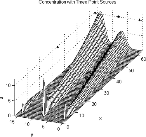
Figure 4. Six sources and nine observations.

Measurement errors in the observations as well as uncertain physical parameters can contribute to significant variation in the computed intensities of the sources. Multiple computations with varying these should be done, and the means and standard deviations should be noted. Large standard deviations from the mean indicate a lack of confidence in the computations. In this case, one must adjust the observation sites, which can be suggested by inspection of the smaller singular values for the least squares matrix and the corresponding columns in V of the singular value decomposition.

Additional information

Funding

No external funding. Some of this research was done before retirement at North Carolina State University.

Notes on contributors

Robert E. White

Professor Robert E. White has published numerous articles on numerical analysis including approximate solutions of partial differential equations, numerical linear algebra, and parallel algorithms. The most recent work is on hazard identification given observation data. He has authored three textbooks. The second edition of Computational Mathematics: Models, Methods and Analysis with MATLAB and MPI will be published in the fall of 2015 by CRC Press/Taylor and Francis.

Appendix 1

Details for Example 3.2 with $n=3$

The least square problem in (11) can be solved for nonnegative $z=H(u)$$$\begin{array}{cc}\hfill z& =(6/5)(data(1)+2data(2))\hfill \\ \hfill & -(16/15)c{u}_1(10-u_1)\hfill \\ \hfill & -(22/15)c{u}_2(10-u_2)\hfill \\ \hfill & -c{u}_3(10-u_3).\hfill \end{array}$$

Next, consider the system in (11). The first two equations give the first and second unknowns in terms of the third unknown$$\begin{array}{cc}\hfill u_1& =\frac{-(3-c10)+\sqrt{{(3-c10)}^2+4c{u}_3}}{2c}\text{and}\hfill \\ \hfill u_2& =\frac{-(3-c10)+\sqrt{{(3-c10)}^2+8c{u}_3}}{2c}.\hfill \end{array}$$

Insert the formulas for $z,u_1$, and $u_2$ into the third equation in the system to get a nonlinear problem for a single unknown $u_3$ and the single equation$$\begin{array}{cc}& \sqrt{{(3-c10)}^2+4c{u}_3}+2\sqrt{{(3-c10)}^2+8c{u}_3}\hfill \\ \hfill & =3(3-c10)+2c(data(1)+2data(2)).\hfill \end{array}$$

When $c=8/100$, this can be solved by Newton’s method to give $u_3=7.2526$. Then solve for the first two unknowns and finally solve for z $$\begin{array}{c}\hfill u_1=2.9748,u_2=5.4952\text{and}z=10.4764.\end{array}$$

In the above example, we were able to explicitly solve for nonnegative z in terms of the components of u. The problem $Au=d(H(u))+\widehat{d}(u)$ is$$\begin{array}{cc}\hfill \left[\begin{array}{ccc}3& 0& -1\\ 0& 3& -2\\ -2& -2& 4\end{array}\right]\left[\begin{array}{c}{u}_1\\ u_2\\ u_3\end{array}\right]& =\left[\begin{array}{c}c{u}_1(10-u_1)\\ c{u}_2(10-u_2)\\ D(u_1,u_2)\end{array}\right]\hfill \end{array}$$

where$$\begin{array}{cc}\hfill D(u_1,u_2)& \equiv (6/5)(data(1)+2data(2))\hfill \\ \hfill & -(16/15)c{u}_1(10-u_1)\hfill \\ \hfill & -(22/15)c{u}_2(10-u_2).\hfill \end{array}$$

The equivalent fixed point problem is $u=A^{-1}(d(H(u))+\widehat{d}(u))$$$\begin{array}{c}\hfill \left[\begin{array}{c}{u}_1\\ u_2\\ u_3\end{array}\right]=(1/18)\left[\begin{array}{ccc}8& 2& 3\\ 4& 10& 6\\ 6& 6& 9\end{array}\right]\left[\begin{array}{c}c{u}_1(10-u_1)\\ c{u}_2(10-u_2)\\ D(u_1,u_2)\end{array}\right]\equiv G(u).\end{array}$$

Expand the matrix-vector product to get$$\begin{array}{c}\hfill G(u)\approx \left[\begin{array}{c}{f}_1(.26)+f_2(-.13)+2.8\\ f_1(-.13)+f_2(.07)+5.6\\ f_1(-.20)+f_2(-.40)+8.4\end{array}\right]\text{where}{f}_i\equiv c{u}_i(10-u_i).\end{array}$$

Assume u, v are nonnegative and bounded and in$$\begin{array}{c}\hfill S\equiv \{u|u={\left[\begin{array}{ccc}{u}_1& u_2& u_3\end{array}\right]}^T,0\le u_i\le 10,i=1,2,3\}.\end{array}$$

Then $0\le f_i\le 25c$ and since $z\ge 0,G(u)\ge 0$. If $c\le 1$, then $G(u)<10$ and G aps S into S.

The contraction mapping theorem requires G(u) to be contractive, that is,$$\begin{array}{c}\hfill {\Vert G(u)-G(v)\Vert }_{\infty }\le r{\Vert u-v\Vert }_{\infty }\text{where}r<1.\end{array}$$

One can approximate the differences$$\begin{array}{cc}\hfill \mathrm{\Delta }{f}_i& \equiv c{u}_i(10-u_i)-c{v}_i(10-v_i)\hfill \\ \hfill \Vert \mathrm{\Delta }{f}_i\Vert & \le c10\Vert u_i-v_i\Vert .\hfill \end{array}$$

Then it is possible to estimate r as a function of c $$\begin{array}{cc}\hfill {\Vert G(u)-G(v)\Vert }_{\infty }& \le \Vert (1/18)\left[\begin{array}{ccc}8& 2& 3\\ 4& 10& 6\\ 6& 6& 9\end{array}\right]\left[\begin{array}{c}\mathrm{\Delta }{f}_1\\ \mathrm{\Delta }{f}_2\\ D(u_1,u_2)-D(v_1,v_2)\end{array}\right]{\Vert }_{\infty }\hfill \\ \hfill & \le (1/18)\Vert \left[\begin{array}{c}\mathrm{\Delta }{f}_1(8+3(-16/15))+\mathrm{\Delta }{f}_2(2+3(-22/15))\\ \mathrm{\Delta }{f}_1(4+6(-16/15))+\mathrm{\Delta }{f}_2(10+6(-22/15))\\ \mathrm{\Delta }{f}_1(6+9(-16/15))+\mathrm{\Delta }{f}_2(6+9(-22/15))\end{array}\right]{\Vert }_{\infty }\hfill \\ \hfill & \le {c10(10.8/18)\Vert u-v\Vert }_{\infty },\hfill \end{array}$$

Let $r=c(108/18)<1$ and require $c<1/6=0.1667$.

References

- Andrle, M., & El Badia, A. (2015). On an inverse problem. Application to a pollution detection problem, II. Inverse Problems in Science and Engineering, 23, 389–412.
- Berman, A., & Plemmons, R. J. (1994). Nonnegative matrices in the mathematical sciences. Philadelphia, PA: SIAM.
- Bjorck, A. (1996). Numerical methods for least squares problems. Philadelphia, PA: SIAM.
- Cryer, C. W. (1971). The solution of a quadratic programming problem using systematic over ralaxation. SIAM Journal on Control and Optimization, 9, 385–392.
- Hamdi, A. (2007). Identification of point sources in two-dimensional advection-diffusion-reaction equations: Application to pollution sources in a river. Stationary case, Inverse Problems in Science and Engineering, 15, 855–870.
- Mahar, P. S., & Datta, B. (1997). Optimal monitoring network and ground-water-pollution source identification. Journal of Water Resources Planning and Management, 199, 199–2007.
- MathWorks Inc. (2015). (123, pp. 199–207). Retrieved from http://www.mathworks.com
- Meyer, C. D. (2000). Matrix analysis and applied linear algebra. Philadelphia, PA: SIAM.
- Pao, C. V. (1992). Nonlinear parabolic and elliptic equations. New York, NY: Plenum Press.
- White, R. E. (2009). Populations with impulsive culling: Identification and control. International Journal of Computer Mathematics, 86, 2143–2164.
- White, R. E. (2011). Identification of hazards with impulsive sources. International Journal of Computer Mathematics, 88, 762–780.
- White, R. E. (2015). MATLAB codes for hazard identification. Retrieved from http://www4.ncsu.edu/eos/users/w/white/www/white/hazardid/hazardid.htm
Appendix 1
Details for Example 3.2 with