Games of entangled agents

Abstract

The paper extends the mathematical formalism of quantum physics to include games of intelligent agents that communicate due to entanglement. The novelty of the approach is based upon a human factor-based behavioral model of an intelligent agent. The model is quantum inspired: it is represented by a modified Madelung equation in which the gradient of quantum potential is replaced by a specially chosen information force. It consists of motor dynamics simulating actual behavior of the agent, and mental dynamics representing evolution of the corresponding knowledge base and incorporating this knowledge in the form of information flows into the motor dynamics. Due to feedback from mental dynamics, the motor dynamics attains quantum-like properties: its trajectory splits into a family of different trajectories, and each of those trajectories can be chosen with the probability prescribed by the mental dynamics; each agent is entangled (in a quantum way) to other agents and makes calculated predictions for future actions; human factor is associated with violation of the second law of thermodynamics: the system can move from disorder to order without external help, and that represents intrinsic intelligence. All of these departures actually extend and complement the classical methods making them especially successful in analysis of communications of agents represented by new mathematical formalism, and in particular, in agent-based economics with a human factor.

Keywords:

• randomness
• stability
• attractors

Public Interest Statement

The novelties introduced in the manuscript, and in particular, departures from Newtonian approach actually extend and complement the classical methods making them especially successful in analysis of communications of agents represented by new mathematical formalism, and in particular, in agent-based economics with a human factor.

1. Introduction

This paper is devoted to a new approach to differential games, (Isaacs, 1965), i.e. to a group of problems related to the modeling and analysis of conflict in the context of a dynamical system. In corresponding agent-based models, the “agents” are “computational objects modeled as interacting according to rules” over space and time, not real people. The rules are formulated to model behavior and social interactions based on incentives and information. Such rules could also be the result of optimization, realized through use of AI methods.

We will concentrate on the non-Newtonian properties of dynamics describing a psychology-based behavior of intelligent agents as players. In other words, we will introduce dynamical systems with a human factor.

1.1. Justification for non-Newtonian approach

All the previous attempts to develop models for so-called active systems (i.e. systems that possess certain degree of autonomy from the environment that allows them to perform motions that are not directly controlled from outside) have been based upon the principles of Newtonian and statistical mechanics. These models appear to be so general that they predict not only physical, but also some biological and economical, as well as social patterns of behavior exploiting such fundamental properties of non-linear dynamics as attractors. Notwithstanding indisputable successes of that approach (neural networks, distributed active systems, etc.), there is still a fundamental limitation that characterizes these models on a dynamical level of description: they propose no difference between a solar system, a swarm of insects, and a stock market. Such a phenomenological reductionism is incompatible with the first principle of progressive biological evolution associated with Darwin. According to this principle, the evolution of living systems is directed toward the highest levels of complexity if the complexity is measured by an irreducible number of different parts, which interact in a well-regulated fashion (although in some particular cases deviations from this general tendency are possible). At the same time, the solutions to the models based upon dissipative Newtonian dynamics eventually approach attractors where the evolution stops while these attractors dwell on the subspaces of lower dimensionality, and therefore, of the lower complexity (until a “master” reprograms the model). Therefore, such models fail to provide an autonomous progressive evolution of living systems (i.e. evolution leading to increase in complexity). Let us now extend the dynamical picture to include thermal forces. That will correspond to the stochastic extension of Newtonian models, while the Liouville equation will extend to the Fokker–Planck equation that includes thermal force effects through the diffusion term. Actually, it is a well-established fact that evolution of life has a diffusion-based stochastic nature as a result of the multi-choice character of behavior of living systems. Such an extended thermodynamics-based approach is more relevant to model of living systems, and therefore, the simplest living species must obey the second law of thermodynamics as physical particles do. However, then the evolution of living systems (during periods of their isolation) will be regressive since their entropy will increase. Therefore, Newtonian physics is not sufficient for simulation the specific properties typical for intelligence.

There is another argument in favor of a non-Newtonian approach to modeling intelligence. As pointed out by Penrose (1955), the Gödel’s famous theorem has the clear implication that mathematical understanding cannot be reduced to a set of known computational rules. That means that no knowable set of purely computational procedures could lead to a computer-control robot that possesses genuine mathematical understanding. In other words, such privileged properties of intelligent systems as common sense, intuition, or consciousness are non-computable within the framework of classical models. That is why a fundamentally new physics is needed to capture these “mysterious” aspects of intelligence, and in particular, to decision-making process.

2. Dynamical model for simulations

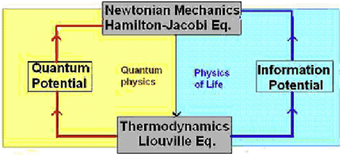
In this section, we review and discuss a behavioral model of intelligent agents, or players. The model is based upon departure from Newtonian dynamics to quantum inspired dynamics that was first introduced in Zak (1998, 2007, 2008, 2014a, 2014b), Figure 1.

Figure 1. Classical physics, quantum physics, and physics of life.

2.1. Destabilizing effect of Liouville feedback

We will start with the derivation of an auxiliary result that illuminates departure from Newtonian dynamics. For mathematical clarity, we will consider here a one-dimensional motion of a unit mass under action of a force f depending upon the velocity v and time t and present it in a dimensionless form(1) $$\dot{v}=f(v,t)$$(1)

referring all the variables to their representative values v₀, t₀, etc.

If initial conditions are not deterministic, and their probability density is given in the form(2) $${\mathit{\rho }}_0={\mathit{\rho }}_0(V),\text{where}\mathit{\rho }\ge 0,\text{and}\underset{-\infty }{\overset{\infty }{\int }}\mathit{\rho }dV=1$$(2)

while ρ is a single-valued function, then the evolution of this density is expressed by the corresponding Liouville equation(3) $$\frac{\mathit{\partial }\mathit{\rho }}{\mathit{\partial }t}+\frac{\mathit{\partial }}{\mathit{\partial }V}(\mathit{\rho }f)=0$$(3)

The solution of this equation subject to initial conditions and normalization constraints (2) determines probability density as a function of V and t:(4) $$\mathit{\rho }=\mathit{\rho }(V,t)$$(4)

Remark. Here and below we make distinction between the random variable v(t) and its values V in probability space.

In order to deal with the constraint (2), let us integrate Equation (3) over the whole space assuming that ρ → 0 at |V| → ∞ and |f| < ∞. Then(5) $$\frac{\mathit{\partial }}{\mathit{\partial }t}\underset{-\infty }{\overset{\infty }{\int }}\mathit{\rho }dV=0,\underset{-\infty }{\overset{\infty }{\int }}\mathit{\rho }dV=\text{const},$$(5)

Hence, the constraint (2) is satisfied for t > 0 if it is satisfied for t = 0.

Let us now specify the force f as a feedback from the Liouville equation

(6) $$f(v,t)=\mathit{\varphi }[\mathit{\rho }(v,t)]$$(6)

and analyze the motion after substituting the force (6) into Equation (2)(7) $$\dot{v}=\mathit{\varphi }[\mathit{\rho }(v,t)],$$(7)

This is a fundamental step in our approach. Although the theory of ODE does not impose any restrictions upon the force as a function of space coordinates, the Newtonian physics does: equations of motion are never coupled with the corresponding Liouville equation. Moreover, it can be shown that such a coupling leads to non-Newtonian properties of the underlying model. Indeed, substituting the force f from Equation (6) into Equation (3), one arrives at the non-linear equation of evolution of the probability density(8) $$\frac{\mathit{\partial }\mathit{\rho }}{\mathit{\partial }t}+\frac{\mathit{\partial }}{\mathit{\partial }V}\{\mathit{\rho }\mathit{\varphi }[\mathit{\rho }(V,t)]\}=0$$(8)

Let us now demonstrate the destabilizing effect of the feedback (6). For that purpose, it should be noticed that the derivative ∂ρ/∂v must change its sign at least once, within the interval −∞ < v < ∞, in order to satisfy the normalization constraint (2).

But since(9) $$Sign\frac{\mathit{\partial }\dot{v}}{\mathit{\partial }v}=Sign\frac{d\mathit{\varphi }}{d\mathit{\rho }}Sign\frac{\mathit{\partial }\mathit{\rho }}{\mathit{\partial }v}$$(9)

there will be regions of v where the motion is unstable, and this instability generates randomness with the probability distribution guided by the Liouville equation (8). It should be noticed that the condition (9) may lead to exponential or polynomial growth of v (in the last case the motion is called neutrally stable, however, as will be shown below, it causes the emergence of randomness as well if prior to the polynomial growth, the Lipcshitz condition is violated).

2.2. Emergence of self-generated stochasticity

In order to illustrate mathematical aspects of the concepts of Liouville feedback in systems under consideration as well as associated with it instability and randomness, let us take the feedback (6) in the form(10) $$f=-{\mathit{\sigma }}^2\frac{\mathit{\partial }}{\mathit{\partial }v}ln\mathit{\rho },$$(10)

to obtain the following equation of motion(11) $$\dot{v}=-{\mathit{\sigma }}^2\frac{\mathit{\partial }}{\mathit{\partial }v}ln\mathit{\rho },$$(11)

This equation should be complemented by the corresponding Liouville equation (in this particular case, the Liouville equation takes the form of the Fokker–Planck equation)(12) $$\frac{\mathit{\partial }\mathit{\rho }}{\mathit{\partial }t}={\mathit{\sigma }}^2\frac{{\mathit{\partial }}^2\mathit{\rho }}{\mathit{\partial }{V}^2}$$(12)

Here v stands for a particle velocity, and σ² is the constant diffusion coefficient.

The solution of Equation (12) subjects to the sharp initial condition(13) $$\mathit{\rho }=\frac{1}{2\mathit{\sigma }\sqrt{\mathit{\pi }t}}exp(-\frac{V^2}{4{\mathit{\sigma }}^{2}t})$$(13)

describes diffusion of the probability density, and that is why the feedback (10) will be called a diffusion feedback.

Substituting this solution with Equation (11) at V = v one arrives at the differential equation with respect to v (t)(14) $$\dot{v}=\frac{v}{2t}$$(14)

and therefore,(15) $$v=C\sqrt{t}$$(15)

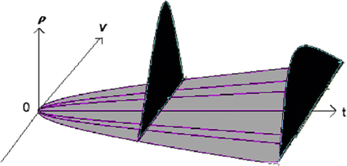
where C is an arbitrary constant. Since v = 0 at t = 0 for any value of C, the solution (15) is consistent with the sharp initial condition for the solution (13) of the corresponding Liouvile equation (12). The solution (15) describes the simplest irreversible motion: it is characterized by the “beginning of time” where all the trajectories intersect (that results from the violation of Lipcsitz condition at t = 0, Figure 2), while the backward motion obtained by replacement of t with (−t) leads to imaginary values of velocities. One can notice that the probability density (13) possesses the same properties.

Figure 2. Stochastic process and probability density.

It is easily verifiable that the solution (15) has the same structure as the solution of the Madelung equation (Zak, 2014b), although the dynamical system (11), (12) is not quantum! The explanation of such a “coincidence” is very simple: the system (11), (12) has the same dynamical topology as that of the Madelung equation where the equation of conservation of the probability is coupled with the equation of conservation of the momentum. As will be shown below, the systems (11), (12) neither quantum nor Newtonian, and we will call such systems quantum-inspired, or self-supervised.

Further analysis of the solution (15) demonstrates that the solution (15) is unstable since

(16) $$\frac{d\dot{v}}{dv}=\frac{1}{2t}>0$$(16)

and therefore, an initial error always grows generating randomness. Initially, at t = 0, this growth is of infinite rate since the Lipchitz condition at this point is violated

(17) $$\frac{d\dot{v}}{dv}\to \infty \text{at}t\to 0$$(17)

This type of instability has been introduced and analyzed in Zak (1992). The unstable equilibrium point (v = 0) has been called a terminal attractor, and the instability triggered by the violation of the Lipchitz condition—a non-Lipchitz instability. The basic property of the non- Lipchitz instability is the following: if the initial condition is infinitely close to the repeller, the transient solution will escape the repeller during a bounded time while for a regular repeller the time would be unbounded. Indeed, an escape from the simplest regular repeller can be described by the exponent v = v₀e^t. Obviously, v → 0 if v₀ → 0, unless the time period is unbounded. On the contrary, the period of escape from the terminal attractor (15) is bounded (and even infinitesimal) if the initial condition is infinitely small, (see Equation (17)).

Considering first Equation (15) at fixed C as a sample of the underlying stochastic process (13), and then varying C, one arrives at the whole ensemble characterizing that process (see Figure 2). One can verify that, as follows from Equation (13), (Risken, 1989), the expectation and the variance of this process are, respectively,(18) $$\overline{v}=0,\tilde{v}=2{\mathit{\sigma }}^{2}t$$(18)

The same results follow from the ensemble (15) at −∞ ≤ C ≤ ∞. Indeed, the first equality in (18) results from symmetry of the ensemble with respect to v = 0; the second one follows from the fact that(19) $$\tilde{v}\propto v^2\propto t$$(19)

It is interesting to notice that the stochastic process (15) is an alternative to the following Langevin equation, (Risken, 1989)(20) $$\dot{v}=\mathrm{\Gamma }(t),\overline{\mathrm{\Gamma }}=0,\tilde{\mathrm{\Gamma }}=\mathit{\sigma }$$(20)

that corresponds to the same Fokker–Planck Equation (12). Here, Γ(t) is the Langevin (random) force with zero mean and constant variance σ.

Thus, the emergence of self-generated stochasticity is the first basic non-Newtonian property of the dynamics with the Liouville feedback.

2.3. Second law of thermodynamics

In order to demonstrate another non-Newtonian property of the systems considered above, let us start with the dimensionless form of the Langevin equation for a one-dimensional Brownian motion of a particle subjected to a random force, (Risken, 1989)(21) $$\dot{v}=-kv+\mathrm{\Gamma }(t),<\mathrm{\Gamma }(t)>=0,<\mathrm{\Gamma }(t)\mathrm{\Gamma }(t^{\prime })>=2\mathit{\sigma }\mathit{\delta }(t-t^{\prime }),[\mathrm{\Gamma }]=1/s$$(21)

Here, v is the dimensionless velocity of the particle (referred to a representative velocity v₀), k is the coefficient of a linear damping force, Γ(t) is the Langevin (random) force per unit mass, σ > 0 is the noise strength. The representative velocity v₀ can be chosen, for instance, as the initial velocity of the motion under consideration.

The corresponding continuity equation for the probability density ρ is the following Fokker–Planck equation(22) $$\frac{\mathit{\partial }\mathit{\rho }}{\mathit{\partial }t}=k\frac{\mathit{\partial }(V\mathit{\rho })}{\mathit{\partial }V}+\mathit{\sigma }\frac{{\mathit{\partial }}^2\mathit{\rho }}{\mathit{\partial }{V}^2},\underset{-\infty }{\overset{\infty }{\int }}\mathit{\rho }dV=1$$(22)

Obviously without external control, the particle cannot escape from the Brownian motion.

Let us now introduce a new force (referred to unit mass and divided by v₀) as a Liouville feedback(23) $$f=\mathit{\sigma }exp\sqrt{D}\frac{\mathit{\partial }}{\mathit{\partial }v}ln\mathit{\rho },[f]=1/s$$(23)

Here D is the dimensionless variance of the stochastic process $D(t)=\underset{-\infty }{\overset{\infty }{\int }}\mathit{\rho }{V}^{2}dV$,

Then the new equation of motion takes the form(24) $$\dot{v}=-kv+\mathrm{\Gamma }(t)+\mathit{\sigma }exp\sqrt{D}\frac{\mathit{\partial }}{\mathit{\partial }v}ln\mathit{\rho },$$(24)

and the corresponding Fokker–Planck equation becomes non-linear(25) $$\frac{\mathit{\partial }\mathit{\rho }}{\mathit{\partial }t}=k\frac{\mathit{\partial }(V\mathit{\rho })}{\mathit{\partial }V}+\mathit{\sigma }(1-exp\sqrt{D})\frac{{\mathit{\partial }}^2\mathit{\rho }}{\mathit{\partial }{V}^2},\underset{-\infty }{\overset{\infty }{\int }}\mathit{\rho }dV=1$$(25)

Obviously, the diffusion coefficient in Equation (25) is negative. Multiplying Equation (25) by V², then integrating it with respect to V over the whole space, one arrives at ODE for the variance $\tilde{v}$(t)(26) $$\dot{D}=2[\mathit{\sigma }(1-exp\sqrt{D})-kD]$$(26)

Thus, as a result of negative diffusion, the variance D monotonously vanishes regardless of the initial value D(0). It is interesting to note that the time T of approaching D = 0 is finite(27) $$T=\frac{1}{2}\underset{D(0)}{\overset{0}{\int }}\frac{dD}{\mathit{\sigma }(1-exp\sqrt{D})-kD}\le \frac{1}{2\mathit{\sigma }}\underset{0}{\overset{\infty }{\int }}\frac{dD}{exp\sqrt{D}-1}=\frac{\mathit{\pi }}{6\mathit{\sigma }}$$(27)

This terminal effect is due to violation of the Lipchitz condition, at D = 0, (Zak, 2014a).

Let us review the structure of the force (23): it is composed only of the probability density and its variance, i.e. out of the components of the conservation Equation (25); at the same time, Equation (25) itself is generated by the equation of motion (24). Consequently, the force (23) is not an external force. Nevertheless, it allows the particle escape from the Brownian motion using its own “internal effort.” It would be reasonable to call the force (23) an information force since it links to information rather than to energy.

Thus, we came across the phenomenon that violates the second law of thermodynamics when the dynamical system moves from disorder to the order without external interactions due to a feedback from the equation of conservation of the probability to the equation of conservation of the momentum. One may ask why the negative diffusion was chosen to be non-linear. Let us turn to a linear version of Equation (26)(28) $$\frac{\mathit{\partial }\mathit{\rho }}{\mathit{\partial }t}=-{\mathit{\sigma }}^2\frac{{\mathit{\partial }}^2\mathit{\rho }}{\mathit{\partial }{V}^2},\underset{-\infty }{\overset{\infty }{\int }}\mathit{\rho }dV=1$$(28)

and discuss a negative diffusion in more detail. As follows from the linear equivalent of Equation (26)(29) $$\dot{D}=-2\mathit{\sigma },\text{i.e.}D=D_0-2\mathit{\sigma }t<0\text{at}t>D_0/(2\mathit{\sigma })$$(29)

Thus, eventually the variance becomes negative, and that disqualifies Equation (29) from being meaningful. As shown in Zak (2014a), the initial value problem for this equation is ill-posed: its solution is not differentiable at any point. Therefore, a negative diffusion must be non-linear in order to protect the variance from becoming negative, Figure 3.

Figure 3. Negative diffusion.

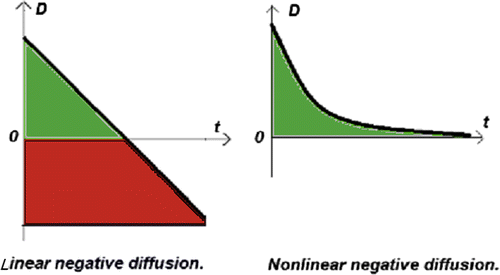
It should be emphasized that negative diffusion represents a major departure from both Newtonian mechanics and classical thermodynamics by providing a progressive evolution of complexity against the second law of thermodynamics.

In the next subsection, we will demonstrate again that formally the dynamics introduced above does not belong to the Newtonian world; nevertheless, its self-supervising capability may associate such a dynamics with a potential model for intelligent behavior. For that purpose, we will turn to even simpler version of this dynamics by removing the external Langevin force and simplifying the information force.

In 1945, Schrödinger wrote in his book “What is life”: “Life is to create order in the disordered environment against the second law of thermodynamics.” The self-supervised dynamical system introduced above is fully consistent with this statement. Indeed, consider a simplified version of Equations (21) and (22)

(30) $$\dot{v}=\mathit{\sigma }\sqrt{D}\frac{\mathit{\partial }}{\mathit{\partial }v}ln\mathit{\rho },$$(30)

(31) $$\frac{\mathit{\partial }\mathit{\rho }}{\mathit{\partial }t}=-\mathit{\sigma }\sqrt{D}\frac{{\mathit{\partial }}^2\mathit{\rho }}{\mathit{\partial }{V}^2},\underset{-\infty }{\overset{\infty }{\int }}\mathit{\rho }dV=1$$(31)

Removal of the Langevin forces makes the particle isolated. Nevertheless, the particle has a capability of moving from disorder to order. For demonstration of this property, we will assume that the Langevin force was suddenly removed at t = 0 so that the initial variance D₀ > 0. Then,(32) $$\dot{D}=-2\mathit{\sigma }\sqrt{D}$$(32) (33) $$whenceD={\left(\sqrt{D_0}-\mathit{\sigma }t\right)}^2$$(33)

As follows from Equation (33), as a result of internal, self-generated force(34) $$F=\mathit{\sigma }\sqrt{D}\frac{\mathit{\partial }}{\mathit{\partial }v}ln\mathit{\rho },$$(34)

the Brownian motion gradually disappears and then vanishes abruptly:(35) $$D\to 0,\dot{D}\to 0,\frac{d\dot{D}}{dD}\to \infty att\to \frac{\sqrt{D_0}}{\mathit{\sigma }}$$(35)

Thus, the probability density shrinks to a delta-function at $t=\frac{\sqrt{D_0}}{\mathit{\sigma }}$. Consequently, the entropy $H(t)=-\underset{V}{\int }\mathit{\rho }ln\mathit{\rho }dV$ decreases down to zero, and that violates the second law of thermodynamics.

Another non-Newtonian property is entanglement.

2.4. Entanglement

In this subsection, we will introduce a fundamental and still mysterious property that was predicted theoretically and corroborated experimentally in quantum systems: entanglement. Quantum entanglement is a phenomenon in which the quantum states of two or more objects have to be described with reference to each other, even though the individual objects may be spatially separated. This leads to correlations between observable physical properties of the systems. As a result, measurements performed on one system seem to be instantaneously influencing other systems entangled with it. Different views of what is actually occurring in the process of quantum entanglement give rise to different interpretations of quantum mechanics. Here, we will demonstrate that entanglement is not a prerogative of quantum systems: it occurs in quantum-inspired (QI) systems that are under consideration in this paper. That will shed light on the concept of entanglement as a special type of global constraint imposed upon a broad class of dynamical systems that include quantum as well as QI systems.

In order to introduce entanglement in QI system, we will start with Equations (11) and (12) and generalize them to the two-dimensional case(36) $${\dot{v}}_1=-a_{11}\frac{\mathit{\partial }}{\mathit{\partial }{v}_1}ln\mathit{\rho }-a_{12}\frac{\mathit{\partial }}{\mathit{\partial }{v}_2}ln\mathit{\rho },$$(36)

(37) $${\dot{v}}_2=-a_{21}\frac{\mathit{\partial }}{\mathit{\partial }{v}_1}ln\mathit{\rho }-a_{22}\frac{\mathit{\partial }}{\mathit{\partial }{v}_2}ln\mathit{\rho },$$(37)

(38) $$\frac{\mathit{\partial }\mathit{\rho }}{\mathit{\partial }t}=a_{11}\frac{{\mathit{\partial }}^2\mathit{\rho }}{\mathit{\partial }{V}^2}+(a_{12}+a_{21})\frac{{\mathit{\partial }}^2\mathit{\rho }}{\mathit{\partial }{V}_1\mathit{\partial }{V}_2}+a_{22}\frac{{\mathit{\partial }}^2\mathit{\rho }}{\mathit{\partial }{V}_2},$$(38)

As in the one- dimensional case, this system describes diffusion without a drift

The solution to Equation (38) has a closed form(39) $$\mathit{\rho }=\frac{1}{\sqrt{2\mathit{\pi }det[{\widehat{a}}_{ij}]t}}exp(-\frac{1}{4t}{b}_{ij}^{\prime }{V}_i{V}_j),i=1,2.$$(39)

Here,(40) $$[b_{ij}^{\prime }]={[{\widehat{a}}_{ij}]}^{-1},{\widehat{a}}_{11}=a_{11},{\widehat{a}}_{22}=a{}_{22},{\widehat{a}}_{12}={\widehat{a}}_{21}=a_{12}+a_{21},{\widehat{a}}_{ij}={\widehat{a}}_{ji},b_{ij}^{\prime }=b_{ji}^{\prime },$$(40)

Substituting the solution (39) with Equations (36) and (37), one obtains(41) $${\dot{v}}_1=\frac{b_{11}{v}_1+b_{12}{v}_2}{2t}$$(41) (42) $${\dot{v}}_2=\frac{b_{21}{v}_1+b_{22}{v}_2}{2t},b_{ij}=b_{ij}^{\prime }{\widehat{a}}_{ij}$$(42)

Eliminating t from these equations, one arrives at an ODE in the configuration space(43) $$\frac{d{v}_2}{d{v}_1}=\frac{b_{21}{v}_1+b_{22}{v}_2}{b_{11}{v}_1+b_{12}{v}_2},v_2\to 0at{v}_1\to 0,$$(43)

This is a classical singular point treated in text books on ODE.

Its solution depends upon the roots of the characteristic equation(44) $${\mathit{\lambda }}^2-2b_{12}\mathit{\lambda }+b_{12}^2-b_{11}{b}_{22}=0$$(44)

Since both the roots are real in our case, let us assume for concreteness that they are of the same sign, for instance, ${\mathit{\lambda }}_1=1,{\mathit{\lambda }}_2=1$. Then the solution to Equation (43) is represented by the family of straight lines(45) $$v_2=\tilde{C}{v}_1,\tilde{C}=const.$$(45)

Substituting this solution into Equation (41) yields (45)(46) $$v_1=C{t}^{\frac{1}{2}(b_{11}+\tilde{C}{b}_{12})}{v}_2=\tilde{C}C{t}^{\frac{1}{2}(b_{11}+\tilde{C}{b}_{12})}$$(46)

Thus, the solutions to Equations (36) and (37) are represented by two-parametrical families of random samples, as expected, while the randomness enters through the time-independent parameters C and $\tilde{C}$that can take any real numbers. Let us now find such a combination of the variables that is deterministic. Obviously, such a combination should not include the random parameters C or $\tilde{C}$. It is easily verifiable that(47) $$\frac{d}{dt}(ln{v}_1)=\frac{d}{dt}(ln{v}_2)=\frac{b_{11}+\tilde{C}{b}_{12}}{2t}$$(47)

and therefore,(48) $$(\frac{d}{dt}ln{v}_1)/(\frac{d}{dt}ln{v}_2)\equiv 1$$(48)

Thus, the ratio (48) is deterministic although both the numerator and denominator are random, (see Equation (47)). This is a fundamental non-classical effect representing a global constraint. Indeed, in theory of stochastic processes, two random functions are considered statistically equal if they have the same statistical invariants, but their point-to-point equalities are not required (although it can happen with a vanishingly small probability). As demonstrated above, the diversion of determinism into randomness via instability (due to a Liouville feedback), and then conversion of randomness to partial determinism (or coordinated randomness) via entanglement is the fundamental non-classical paradigm that may lead to instantaneous transmission of conditional information on remote distance that to be discussed below.

2.5. Relevance to model of intelligent agents

The model under discussion was inspired by E. Schrödinger, the creator of quantum mechanics who wrote in his book “What is Life”: “Life is to create order in the disordered environment against the second law of thermodynamics.” The proposed model illuminates the “border line” between living and non-living systems. The model introduces a biological particle that, in addition to Newtonian properties, possesses the ability to process information. The probability density can be associated with the self-image of the biological particle as a member of the class to which this particle belongs, while its ability to convert the density into the information force—with the self-awareness (both these concepts are adopted from psychology). Continuing this line of associations, the equation of motion (such as Equations (1) or (7)) can be identified with a motor dynamics, while the evolution of density (see Equations (3) or (8)—with a mental dynamics. Actually, the mental dynamics plays the role of the Maxwell sorting demon: it rearranges the probability distribution by creating the information potential and converting it into a force that is applied to the particle. One should notice that mental dynamics describes evolution of the whole class of state variables (differed from each other only by initial conditions), and that can be associated with the ability to generalize that is a privilege of living systems. Continuing our biologically inspired interpretation, it should be recalled that the second law of thermodynamics states that the entropy of an isolated system can only increase. This law has a clear probabilistic interpretation: increase of entropy corresponds to the passage of the system from less probable to more probable states, while the highest probability of the most disordered state (that is the state with the highest entropy) follows from a simple combinatorial analysis. However, this statement is correct only if there is no Maxwell’ sorting demon, i.e. nobody inside the system is rearranging the probability distributions. But this is precisely what the Liouville feedback is doing: it takes the probability density ρ from Equation (3), creates functionals and functions of this density, converts them into a force and applies this force to the equation of motion (1). As already mentioned above, because of that property of the model, the evolution of the probability density becomes non-linear, and the entropy may decrease “against the second law of thermodynamics,” Figure 4.

Figure 4. Living system: Deviation from classical thermodynamics.

Obviously the last statement should not be taken literary; indeed, the proposed model captures only those aspects of the living systems that are associated with their behavior, and in particular, with their motor–mental dynamics, since other properties are beyond the dynamical formalism. Therefore, such physiological processes that are needed for the metabolism, reproduction, est., are not included into the model. That is why this model is in a formal disagreement with the first and second laws of thermodynamics while the living systems are not. Indeed, applying the first law of thermodynamics we imply violation of conservation of mechanical energy since other types of energies (chemical, electro-magnetic, etc.) are beyond our mathematical formalism. Applying the second law of thermodynamics, we consider our system as isolated one while the underlying real system is open due to other activities of livings that were not included in our model. Nevertheless, despite these limitations, the proposed model captures the “magic” of life: the ability to create self-image and self-awareness, and that fits perfectly to the concept of intelligent agent. Actually, the proposed model represents governing equations for interactions of intelligent agents. In order to emphasize the autonomy of the agents’ decision-making process, we will associate the proposed models with self-supervised (SS) active systems.

By an active system, we will understand here a set of interacting intelligent agents capable of processing information, while an intelligent agent is an autonomous entity, which observes and acts upon an environment and directs its activity toward achieving goals. The active system is not derivable from the Lagrange or Hamilton principles, but it is rather created for information processing. One of the specific differences between active and physical systems is that the former are supposed to act in uncertainties originated from incompleteness of information. Indeed, an intelligent agent almost never has access to the whole truth of its environment. Uncertainty can also arise because of incompleteness and incorrectness in the agent’s understanding of the properties of the environment. That is why QI SS systems are well suited for representation of active systems.

2.6. Self-supervised active systems with integral feedback

In this subsection, we will introduce a feedback from the mental to motor dynamics that is different from the feedback (6) discussed above. This feedback will make easier to formulate new principles of the competitive mode of agents associated with game theory.

Let us introduce the following feedback, (Zak, 2008)(49) $$f=\frac{1}{\mathit{\rho }(v,t)}\underset{-\infty }{\overset{v}{\int }}[\mathit{\rho }(\mathit{\zeta },t)-{\mathit{\rho }}^{*}(\mathit{\zeta })]dv$$(49)

With the feedback (49), Equations (7) and (8) take the form, respectively,(50) $$f=\frac{1}{\mathit{\rho }(v,t)}\underset{-\infty }{\overset{v}{\int }}[\mathit{\rho }(\mathit{\zeta },t)-{\mathit{\rho }}^{*}(\mathit{\zeta })]dv$$(50)

(51) $$\frac{\mathit{\partial }\mathit{\rho }}{\mathit{\partial }t}+\mathit{\rho }(t)-{\mathit{\rho }}^{*}=0$$(51)

The last equation has the analytical solution(52) $$\mathit{\rho }=({\mathit{\rho }}_0-{\mathit{\rho }}^{*})e^{-t}+{\mathit{\rho }}^{*}$$(52)

Subject to the initial condition(53) $$\mathit{\rho }(t=0)={\mathit{\rho }}_0$$(53)

This solution converges to a prescribed, or target, stationary distribution ρ^*(V). Obviously the normalization condition for ρ is satisfied if it is satisfied for ρ₀ and ρ^*. This means that Equation (51) has an attractor in the probability space, and this attractor is stochastic. Substituting the solution (52) with Equation (50), one arrives at the ODE that simulates the stochastic process with the probability distribution (52)(54) $$\dot{v}=\frac{e^{-t}}{[{\mathit{\rho }}_0(v)-{\mathit{\rho }}^{*}(v)]e^{-t}+{\mathit{\rho }}^{*}(v)}\underset{-\infty }{\overset{v}{\int }}[{\mathit{\rho }}_0(\mathit{\zeta })-{\mathit{\rho }}^{*}(\mathit{\zeta })]d\mathit{\zeta }$$(54)

As notices above, the randomness of the solution to Equation (54) is caused by instability that is controlled by the corresponding Liouville equation. It should be emphasized that in order to run the stochastic process started with the initial distribution ρ₀ and approaching a stationary process with the distribution ρ^*, one should substitute into Equation (54) the analytical expressions for these functions.

It is reasonable to assume that the solution (4) starts with sharp initial condition(55) $${\mathit{\rho }}_0(V)=\mathit{\delta }(V)$$(55)

As a result of that assumption, all the randomness is supposed to be generated only by the controlled instability of Equation (54). Substitution of Equation (55) into Equation (54) leads to two different domains of v: v ≠ 0 and v = 0 where the solution has two different forms, respectively,(56) $$\underset{-\infty }{\overset{v}{\int }}{\mathit{\rho }}^{*}(\mathit{\zeta })d\mathit{\zeta }=\frac{C_1}{e^{-t}-1},v\ne 0$$(56)

(57) $$v\equiv 0$$(57)

Equation (57) represents a singular solution, while Equation (56) is a regular solution that include arbitrary constant C. The regular solutions is unstable at t = 0, |v| → 0 where the Lipschitz condition is violated(58) $$\frac{d\dot{v}}{dv}\to \infty att\to 0,|v|\to 0$$(58)

and therefore, an initial error always grows generating randomness.

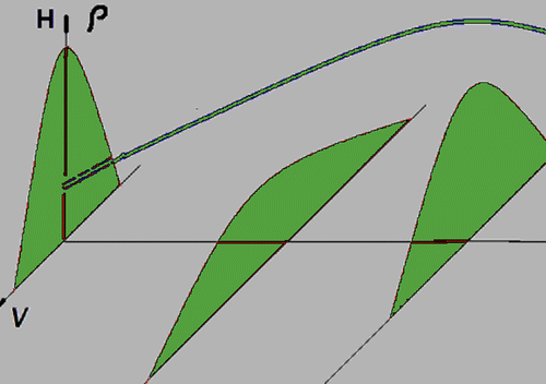
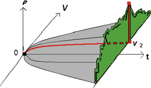
Let us analyze the behavior of the solution (56) in more detail. As follows from this solution, all the particular solutions intersect at the same point v = 0 at t = 0, and that leads to non-uniqueness of the solution due to violation of the Lipcshitz condition. Therefore, the same initial condition v = 0 at t = 0 yields infinite number of different solutions forming a family (56); each solution of this family appears with a certain probability guided by the corresponding Liouville equation (51). For instance, in cases plotted in Figures 5 and 6, the “winner” solution is, respectively,(59) $$v_1=\mathit{\epsilon }\to 0,\mathit{\rho }(v_1)={\mathit{\rho }}_{max},\text{and}v=v_2,\mathit{\rho }(v_2)=sup\{\mathit{\rho }\}$$(59)

Figure 5. Stochastic process and probability density.

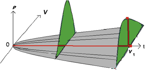
Figure 6. Global maximum.

since it passes through the maximum of the probability density (51). However, with lower probabilities, other solutions of the family (53) can appear as well. Obviously, this is a non-classical effect. Qualitatively, this property is similar to those of quantum mechanics: the system keeps all the solutions simultaneously and displays each of them “by a chance,” while that chance is controlled by the evolution of probability density (51).

The approach is generalized to n-dimensional case simply by replacing v with a vector v = v₁, v₂, … v_n since Equation (51) does not include space derivatives.

Examples. Let us start with the following normal distribution(60) $${\mathit{\rho }}^{*}(V)=\frac{1}{\sqrt{2\mathit{\pi }}}{e}^{-\frac{V^2}{2}}$$(60)

Substituting the expression (60) and (55) with Equation (56) at V = v, one obtains(61) $$v=er{f}^{-1}(\frac{C_1}{e^{-t}-1}),v\ne 0$$(61)

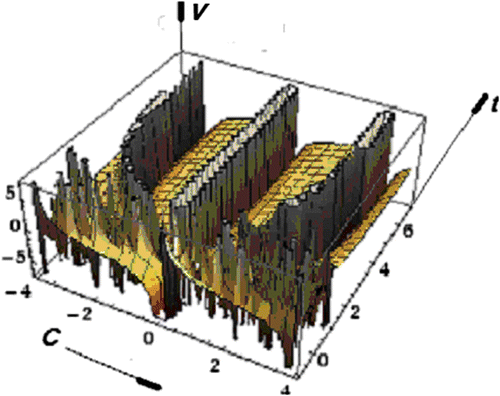
As another example, let us choose the target density ρ^* as the student’s distribution, or so called power law distribution(62) $${\mathit{\rho }}^{*}(V)=\frac{\mathrm{\Gamma }(\frac{\mathit{\nu }+1}{2})}{\sqrt{\mathit{\nu }\mathit{\pi }}\mathrm{\Gamma }(\frac{\mathit{\nu }}{2})}{(1+\frac{V^2}{\mathit{\nu }})}^{-(\mathit{\nu }+1)/2}$$(62)

Substituting the expression (62) with Equation (56) at V = v, and ν = 1, one obtains(63) $$v=tan(\frac{C}{e^{-t}-1})forv\ne 0$$(63)

The 3D plot of the solutions of Equations (61) and (63), are presented in Figures 7, and 8 respectively.

Figure 7. Dynamics driving random events to normal distribution.

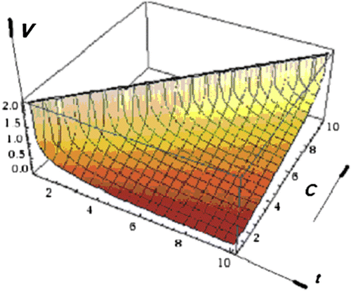
Figure 8. Dynamics driving random events to power law.

2.7. Finding global maximum

Based upon the proposed model with integral feedback, a simple algorithm for finding a global maximum of an n-dimensional function can be formulated. The idea of the proposed algorithm is very simple: based upon the model with integral feedback (50), and (51), introduce a positive function $\mathit{\psi }(v_1,v_2,...v_n),|v_i|<\infty$ to be maximized as the probability density ρ^*(v₁, v₂, ...v_n) to which the solution of Equation (50) is attracted. Then the larger value of this function will have the higher probability to appear. The following steps are needed to implement this algorithm.

(1)	Build and implement the n-dimensional version of the model Equations (50), and (51), as an analog devise(64) $${\dot{v}}_i=\frac{e^{-t}}{n\{[{\mathit{\rho }}_0(v)-{\mathit{\rho }}^{*}(v)]e^{-t}+{\mathit{\rho }}^{*}(v)\}}\underset{-\infty }{\overset{v_i}{\int }}[{\mathit{\rho }}_0(\mathit{\zeta })-{\mathit{\rho }}^{*}(\mathit{\zeta }{)]}^{}d\mathit{\zeta },i=1,2,\dots n.$$(64)
(2)	Normalize the function to be maximized(65) $$\overline{\mathit{\psi }}(\{v\})=\frac{\mathit{\psi }(\{v\})}{\underset{-\infty }{\overset{\infty }{\int }}\mathit{\psi }(\{v\})d\{v\}}$$(65)
(3)	Using Equation (51), evaluate time τ of approaching the stationary process to accuracy ε(66) $$\mathit{\tau }\approx ln\frac{1-\overline{\mathit{\psi }}}{\mathit{\epsilon }\overline{\mathit{\psi }}}$$(66)
(4)	Substitute $\overline{\mathit{\psi }}$ instead of ρ* with Equations (64) and run the system during the time interval τ.
(5)	The solution will “collapse” into one of possible solutions with the probability $\overline{\mathit{\psi }}$.Observing (measuring) the corresponding values of {v*}, find the first approximation to the optimal solution.
(6)	Switching the device to the initial state and then starting again, arrive at the next approximations.
(7)	The sequence of the approximations represents Bernoulli trials that exponentially improve the chances of the optimal solution to become a winner. Indeed, the probability of success ρs and failure ρf after the first trial are, respectively,(67) $${\mathit{\rho }}_s={\overline{\mathit{\psi }}}_1,{\mathit{\rho }}_f=1-{\overline{\mathit{\psi }}}_1$$(67) Then the probability of success after M trials is(68) $${\mathit{\rho }}_{sM}=1-{(1-\overline{\mathit{\psi }})}^M\to 1atM\to \infty$$(68) Therefore, after polynomial number of trials, one arrived at the solution to the problem (unless the function ψ is flat).

The main advantage of the proposed methodology is in a weak restriction imposed upon the space structure of the function $\overline{\mathit{\psi }}(\{v\})$: it should be only integrable since there is no space derivatives included in the model (64). This means that $\overline{\mathit{\psi }}(\{v\})$ is not necessarily to be differentiable. For instance, it can be represented by a Weierstrass-like function $f(v)={\sum }_0^{\infty }{a}^{n}cos(b^n\mathit{\pi }v)$, where 0 < a < 1, b is a positive odd integer, and ab > 1 + 1.5π.

In a particular case when $\overline{\mathit{\psi }}(\{x\})$ is twice differentiable, the algorithm is insensitive to local maxima because it is driven not by gradients, but by the values of this function.

2.8. Entanglement in QI active systems with integral feedback

We will continue the analysis of the QI system with integral feedback introduced above proceeding with the two-dimensional case(69) $${\dot{v}}_1=\frac{1}{2\mathit{\rho }(v_1,v_2,t)}\underset{-\infty }{\overset{v_1}{\int }}[\mathit{\rho }(\mathit{\eta },v_2,t)-{\mathit{\rho }}^{*}(\mathit{\eta },v_2)]d\mathit{\eta }$$(69) (70) $${\dot{v}}_2=\frac{1}{2\mathit{\rho }(v_1,v_2,t)}\underset{-\infty }{\overset{v_2}{\int }}[\mathit{\rho }(v_1,\mathit{\eta },t)-{\mathit{\rho }}^{*}(v_1,\mathit{\eta })]d\mathit{\eta }$$(70) (71) $$\frac{\mathit{\partial }\mathit{\rho }(V,t)}{\mathit{\partial }t}+\mathit{\rho }(V,t)-{\mathit{\rho }}^{*}(V)=0$$(71)

The solution of Equation (71) has the same form as for one-dimensional case, (see Equation (52))(72) $$\mathit{\rho }={\mathit{\rho }}_0+{\mathit{\rho }}^{*}(1-e^{-t})$$(72)

Substitution this solution into Equations (69) and (70), yields, respectively,(73) $${\dot{v}}_1=\frac{e^{-t}}{2[{\mathit{\rho }}_0(v_1,v_2)-{\mathit{\rho }}^{*}(v_1,v_2)]e^{-t}+{\mathit{\rho }}^{*}(v_1,v_2)}\underset{-\infty }{\overset{v_1}{\int }}[{\mathit{\rho }}_0(\mathit{\eta },v_2)-{\mathit{\rho }}^{*}(\mathit{\eta },v_2)]d\mathit{\eta }$$(73)

(74) $${\dot{v}}_2=\frac{e^{-t}}{2[{\mathit{\rho }}_0(v_1,v_2)-{\mathit{\rho }}^{*}(v_1,v_2)]e^{-t}+{\mathit{\rho }}^{*}(v_1,v_2)}\underset{-\infty }{\overset{v_2}{\int }}[{\mathit{\rho }}_0(v_1,\mathit{\eta })-{\mathit{\rho }}^{*}(v_1,\mathit{\eta })]d\mathit{\eta }$$(74)

that are similar to Equation (54). Following the same steps as in one-dimensional case, one arrives at the following solutions of Equations (73) and (74), respectively,(75) $$\underset{-\infty }{\overset{v_1}{\int }}{\mathit{\rho }}^{*}(\mathit{\eta },v_2)d\mathit{\eta }=\frac{C_1}{e^{-t}-1},v_1\ne 0$$(75) (76) $$\underset{-\infty }{\overset{v_2}{\int }}{\mathit{\rho }}^{*}(\mathit{\eta },v_1)d\mathit{\eta }=\frac{C_2}{e^{-t}-1},v_2\ne 0$$(76)

that are similar to the solution (56). Since ρ(v₁, v₂) is the known (preset) function, Equations (75) and (76) implicitly define v₁ and v₂ as functions of time. Eliminating time t and orbitary constants C₁, C₂, one obtains(77) $$\frac{d}{dt}[ln\underset{-\infty }{\overset{v_1}{\int }}{\mathit{\rho }}^{*}(\mathit{\eta },v_2)d\mathit{\eta }]/\frac{d}{dt}[ln\underset{-\infty }{\overset{v_2}{\int }}{\mathit{\rho }}^{*}(v_1,\mathit{\eta })d\mathit{\eta }]\equiv 1$$(77)

Thus, the ratio (77) is deterministic although both the numerator and denominator are random, (see Equations (75) and (66)).

3. Application to games of entangled agents

In this section, we will address a situation when agents are competing. That means that they have different objectives. Turning to Equation (75), (76), one can rewrite them for the case of competing agents(78) $${\dot{v}}_i=\frac{1}{n\mathit{\rho }(v_{1,}\dots v_n,t)}\underset{-\infty }{\overset{v_i}{\int }}[\mathit{\rho }({\mathit{\zeta }}_i,v_{j\ne i},t)-{\mathit{\rho }}_i^{*}({\mathit{\zeta }}_i,v_{j\ne i})]d{\mathit{\zeta }}_i$$(78)

(79) $$\frac{d\mathit{\rho }}{dt}+\mathit{\rho }(t)-\frac{1}{n}\sum _1^n{a}_k{\mathit{\rho }}_k^{*}=0,\sum _{k=1}^n{a}_k=n{\mathit{\rho }}_i^{*}\ne {\mathit{\rho }}_j^{*}ifi\ne j.$$(79)

where ${\mathit{\rho }}_k^{*}$ is the preset density of the kth agent that can be considered as his objective, a_k is a constant weight of the kth agent’s effort to approach his objective.

Thus, each kth agent is trying to establish his own static attractor ${\mathit{\rho }}_k^{*}$, but due to entanglement, the whole system will approach the weighted average(80) $$\mathit{\rho }=[{\mathit{\rho }}^0-\frac{1}{n}\sum _{i=1}^n(a_i{\mathit{\rho }}_i^{*})]e^{-t}+\frac{1}{n}\sum _{i=1}^n{a}_i{\mathit{\rho }}_i^{*}$$(80)

$$\mathit{\rho }(t)=\frac{1}{n}\sum _1^n{a}_k{\mathit{\rho }}_k^{*}\text{at}t\to \infty$$

Substituting the solution (80) with Equation (78), one arrives at a coupled system of n ODE with respect to n state variables v_i. Although a closed form analytical solution of the system (78) and (79) is not available, its property of the Lipcshitz instability at t = 0 could be verified. This means that the solution to the system (78) and (79) is random, and if the system is run many times, the statistical properties of the whole ensemble will be described by Equation (80). Obviously, those agents who have chosen density with a sharp maximum are playing more risky game. Here, we have assumed that competing agents are still entangled, and therefore, their information about each other is complete. More complex situation when the agents are not entangled, and exchanged information is incomplete is address in the next section. The simplest way to formalize the incompleteness of information possessed by competing agent is to include the “vortex” terms into Equation (77): these terms could change each particular trajectory of the agent motion, but they would not change the statistical invariants that remain available to the competing agents(81) $${\dot{v}}_i=\frac{1}{n\mathit{\rho }(v_{1,}\dots v_n,t)}[\underset{-\infty }{\overset{v_i}{\int }}[\mathit{\rho }({\mathit{\zeta }}_i,v_{j\ne i},t)-{\mathit{\rho }}^{*}({\mathit{\zeta }}_i,v_{j\ne i})]d{\mathit{\zeta }}_i+\sum _{j\ne i}^n{T}_{ij}tanh{v}_j]$$(81)

It is easily verifiable that the augmented neural net-like terms do not effect the corresponding Liouville equation, and therefore, they do not change the static attractor in the probability space described by Equation (76). However, they may significantly change the configuration of the random trajectories in physical space making their entanglement more sophisticated. Another way to formalize uncertainty is to introduce a complex joint probability density where its imaginary part represents a measure of uncertainty in density distribution. This case will be considered below in more details.

3.1. Problem formulation

In this section, we will present a draft of application of self-supervised active dynamical systems to differential games. Following von-Neuman, and Isaaks, (Isaacs, 1965), we will introduce a two-player zero-sum (antagonistic) differential game that is described by dynamical Equation (64) rewritten for i = 1,2(82) $${\dot{v}}_i=\frac{1}{2\mathit{\rho }(v_{1,}...v_n,t)}\underset{-\infty }{\overset{v_i}{\int }}[\mathit{\rho }({\mathit{\zeta }}_i,v_{j\ne i},t)-a_i{C}_i{f}_i({\mathit{\zeta }}_i,v_{j\ne i})]d{\mathit{\zeta }}_i{f}_1=f,f_2=f^{-1},a_1+a_2=2.$$(82)

where v is the state vector, f₁ is the control vector of the maximizing player E (evader), f₂ is the control vector of the minimizing player P (pursuer), and C₁, C₂are the normalizing factors. Obviously, f is a known function of both state variables.

However, the rules of the game we propose is slightly different from those introduced by Isaaks, namely: the player P tries to minimize the function f, (i.e. maximize the function f⁻¹) while the player E tries to maximize f in the same manner as it was described in the previous subsection i.e. via entanglement. The Liouville equation for the system (69) follows from Equation (79)

(83) $$\frac{d\mathit{\rho }}{dt}+\mathit{\rho }(t)-\frac{1}{2}(a_1{C}_{1}f+a_2{C}_2{f}^{-1})=0$$(83)

whence(84) $$\mathit{\rho }=[{\mathit{\rho }}^0-\frac{1}{2}(a_1{C}_{1}f+a_2{C}_2{f}^{-1})]e^{-t}+\frac{1}{2}(a_1{C}_{1}f+a_2{C}_2{f}^{-1}),$$(84)

We will now give a description of the game.

The game starts with zero initial conditions:(85) $$v_1=0,v_2=0,{\mathit{\rho }}^0=\mathit{\delta }(v_1,v_2)att=0$$(85)

It is assumed that each player has access to the systems (82), (84), and therefore, he has complete information about its state. The substitution of Equation (84) with Equation (82) closes the system (82). However, because of a failure of the Lipcshitz condition at t = 0 (see Equation (58)), the solution of Equation (82) is random, and each player can predict it only in terms of probability. As follows from Equation (84), the highest probability to appear has the solution that delivers the global maximum to the payoff function(86) $$F=a_1{C}_{1}f+a_2{C}_2{f}^{-1}$$(86)

Obviously, the player that has higher weight a_i would have better chances to win since the global maximum of Equation (86) is closer to the global maximum of his goal function. With reference to Equation (86), a player can evaluate time τ of approaching the stationary process to accuracy ε as(87) $$\mathit{\tau }\approx ln\frac{1-F}{\mathit{\epsilon }F}$$(87)

and introduce(88) $$v_1^1=v_1(\mathit{\tau }),v_2^1(\mathit{\tau }),f_1^1=f_1(v_1^1,v_2^2),f_2^1=f_2(v_1^1,v_2^1)$$(88)

This is the end of the first move. After that, each player updates his weight as following(89) $$a_1^1=a_1+\frac{f_1^1-f_1^0}{f_1^0},a_2^1=a_2-\frac{f_1^1-f_1^0}{f_1^0},f_1^0\ne 0,$$(89)

and starts the next move with the same initial conditions (85). But the system (82), (84) is different now: the control functions f₁, f₂ are to be replaced by their updated values $f_1^1,f_2^1$, respectively. Thus, during the first move, the potential winner is selected by a chance, and during the next move, his chances are increased due to favorable update of the weights. However, the role of the chance is still significant even during the subsequent moves; indeed, if the global maximum of the control function F is sharp, the initially selected potential winner still can lose.

The game ends when one of the players achieves his goal my maximizing his control function to a preset level, for instance, if(90) $$f_1-f_2>A^2$$(90)

3.2. Games with incomplete information

The theory presented above includes applications to such problems as battle games, games with moving craft, pursuit games, etc. However, the main limitation of this theory, as well as the most of the game theories, is that it requires complete information about the state variables available to both players. This limitation significantly diminishes the applicability of the theory to real-life games where the complete information is not available. That is why the extension of this theory to cases of incomplete information is of vital importance. In our application, we will assume that each player knows only his own state variables, while he has to guess about the state variables of his adversary. For that case, the mathematical formalism of QI systems can offer a convenient tool to replace unknown value of a state variable by its expected value. Such a possibility is available due to players’ dependence (but not necessarily entanglement) via the joint probability density: since each player possesses the joint density, he can, at any moment, compute the expected value of the state variable of the other player.

We assume that the players follow the strategy: “what do you think I think you think …?” and we will start with the assumption that each player takes a conservative view by thinking that although he does not know the values of the state variable of his adversary, the adversary does know the values of his state variable. Then the governing equation for the Evader will be(91) $${\dot{v}}_1=\frac{1}{2\mathit{\rho }(v_{1,}{\overline{V}}_2,t)}\underset{-\infty }{\overset{v_1}{\int }}\mathit{\rho }({\mathit{\zeta }}_1,{\overline{V}}_2,t)-a_1{C}_1{f}_1({\mathit{\zeta }}_1,{\overline{V}}_2)d{\mathit{\zeta }}_1$$(91)

Here ${\overline{V}}_2$ is the expected value of V₂(92) $${\overline{V}}_2=\underset{-\infty }{\overset{\infty }{\int }}{V}_2\mathit{\rho }(V_1,V_2)d{V}_{1}d{V}_2$$(92)

Now the Evader has to create the image of the Pursuer using the expected value of his state variable(93) $${\dot{v}}_{2|1}=\frac{1}{2\mathit{\rho }(v_{1,}{\overline{V}}_2,t)}\underset{-\infty }{\overset{v_2}{\int }}[\mathit{\rho }(v_1,{\mathit{\zeta }}_2,t)-a_2{C}_2{f}_2(v_1,{\mathit{\zeta }}_2)]d{\mathit{\zeta }}_2$$(93)

where v_2|1 is the state variable of the Pursuer in view of the Evader.

The corresponding Liouville equation that governs the joint probability equation is not changed: it is still given by Equation (79). Its solution (84) should be substituted with Equations (91) and (93) along with the Equation (92). Obviously, the expected value (92) is found from the solution (84)(94) $${\overline{V}}_i=[{\overline{V}}_i^0-\underset{-\infty }{\overset{\infty }{\int }}d{\mathit{\zeta }}_1\underset{-\infty }{\overset{\infty }{\int }}d{\mathit{\zeta }}_2\{[\frac{1}{2}(a_1{C}_{1}f+a_2{C}_2{f}^{-1})]e^{-t}+\frac{1}{2}(a_1{C}_{1}f+a_2{C}_2{f}^{-1})]{\overline{V}}_i\},i=1,2.$$(94)

The system of Equations (91), (93), and (79) with reference to Equations (92), (94) is closed.

Similar system can be obtained for governing equation of the Pursuer coupled with the governing equation of his image of the Evador:(95) $${\dot{v}}_2=\frac{1}{2\mathit{\rho }({\overline{V}}_1,v_2,t)}\underset{-\infty }{\overset{v_1}{\int }}\mathit{\rho }({\overline{V}}_1,{\mathit{\zeta }}_2,t)-a_2{C}_2{f}_2({\overline{V}}_1,{\mathit{\zeta }}_2)d{\mathit{\zeta }}_2$$(95)

(96) $${\dot{v}}_{1|2}=\frac{1}{2\mathit{\rho }({\overline{V}}_1,v_2,t)}\underset{-\infty }{\overset{v_1}{\int }}\mathit{\rho }({\mathit{\zeta }}_1,v_2,t)-a_2{C}_2{f}_2({\mathit{\zeta }}_1,v_2)d{\mathit{\zeta }}_1$$(96)

(97) $${\overline{V}}_1=\underset{-\infty }{\overset{\infty }{\int }}{V}_1\mathit{\rho }(V_1,V_2)d{V}_{1}d{V}_2$$(97)

After substitution of Equation (79) with Equations (95) and (96), with reference to Equations (97) and (94), one arrives at the closed system.

Thus, we obtain two independent systems of ODE describing entanglement of the player with the image of his adversary. Each system has random solutions that appear with the probability described by Equation (79). After time interval τ (see Equation (87)), each player gets access to the real values of the functions f_i to be maximized, and based upon that, he can update the state variables and weights for the next move, (see Equations (88) and (89)).

Let us consider now the case when the players do not know the values of state variables of their adversary.

Then instead of the systems (91), (93), and (95), (96) we have, respectively(98) $${\dot{v}}_1=\frac{1}{2\mathit{\rho }(v_{1,}{\overline{V}}_2,t)}\underset{-\infty }{\overset{v_1}{\int }}\mathit{\rho }({\mathit{\zeta }}_1,{\overline{V}}_2,t)-a_1{C}_1{f}_1({\mathit{\zeta }}_1,{\overline{V}}_2)d{\mathit{\zeta }}_1$$(98)

(99) $${\dot{v}}_{2|1|1}=\frac{1}{2\mathit{\rho }({\overline{V}}_{1,}{\overline{V}}_2,t)}\underset{-\infty }{\overset{v_2}{\int }}[\mathit{\rho }({\overline{V}}_1,{\mathit{\zeta }}_2,t)-a_2{C}_2{f}_2({\overline{V}}_1,{\mathit{\zeta }}_2)]d{\mathit{\zeta }}_2$$(99)

(100) $${\dot{v}}_2=\frac{1}{2\mathit{\rho }({\overline{V}}_1,v_2,t)}\underset{-\infty }{\overset{v_1}{\int }}\mathit{\rho }({\overline{V}}_1,{\mathit{\zeta }}_2,t)-a_2{C}_2{f}_2({\overline{V}}_1,{\mathit{\zeta }}_2)d{\mathit{\zeta }}_2$$(100)

(101) $${\dot{v}}_{1||2|2}=\frac{1}{2\mathit{\rho }({\overline{V}}_1,{\overline{V}}_2,t)}\underset{-\infty }{\overset{v_1}{\int }}\mathit{\rho }({\mathit{\zeta }}_1,{\overline{V}}_2,t)-a_2{C}_2{f}_2({\mathit{\zeta }}_1,{\overline{V}}_2)d{\mathit{\zeta }}_1$$(101)

Here, v_2|1|1 is the state variable of the Pursuer’s view on the Evader in view of the Pursuer, and v_1|2|2 is the state variable of the Evader’s view on the Pursuer in view of the Evader.

It is easy to conclude that the image Equations (99) and (101) can be solved independently(102) $$v_{2|1|1}=\underset{0}{\overset{t}{\int }}dt\frac{1}{2\mathit{\rho }({\overline{V}}_{1,}{\overline{V}}_2,t)}\underset{-\infty }{\overset{v_2}{\int }}[\mathit{\rho }({\overline{V}}_1,{\mathit{\zeta }}_2,t)-a_2{C}_2{f}_2({\overline{V}}_1,{\mathit{\zeta }}_2)]d{\mathit{\zeta }}_2$$(102)

(103) $$v_{1|2|2}=\underset{0}{\overset{t}{\int }}dt\frac{1}{2\mathit{\rho }({\overline{V}}_1,{\overline{V}}_2,t)}\underset{-\infty }{\overset{v_1}{\int }}\mathit{\rho }({\mathit{\zeta }}_1,{\overline{V}}_2,t)-a_2{C}_2{f}_2({\mathit{\zeta }}_1,{\overline{V}}_2)d{\mathit{\zeta }}_1$$(103)

Now replacing ${\overline{V}}_2,{\overline{V}}_1$ in Equations (98) and (100) by the solutions for v_2|1|1 and v_1|2|2, respectively, one arrives at two independent ODE describing behaviors of the players. Therefore, at this level of incompleteness of information, the entanglement disappears.

The games with incomplete information give a reason to distinguish two type of dependence between the agents described by the variables v_i in the iQ systems. The first type of dependence is entanglement that has been introduced and discussed above. One should recall that in order to be entangled, the agents are supposed to run the system jointly during some initial period of time. But what happens if the agents had never been in contact? Obviously they are not entangled, i.e. they cannot predict each other’s motions. However, they are not completely independent: they can make random decisions, but the probability of these decisions will be correlated via the joint probability. As a result, the agents will be able to predict expected decisions of each other. We will call such correlation a weak entanglement. As follows from the games with incomplete information considered above, weak entanglement was presented as entanglement of an agent with the probabilistic image of another agent.

4. Games of partially entangled agents

In this section we introduce a new, more sophisticated entanglement that does not exist in quantum mechanics, but can be found in QI models. This finding is based upon existence of incompatible stochastic processes that are considered below.

4.1. Incompatible stochastic processes

Classical probability theory defines conditional probability densities based upon the existence of a joint probability density. However, one can construct correlated stochastic processes that are represented only by conditional densities since a joint probability density does not exist. For that purpose, consider two coupled Langevin equations (Risken, 1989)(104) $${\dot{x}}_1=g_{11}(x_2)L_1(t)$$(104) (105) $${\dot{x}}_2=g_{22}(x_1)L_2(t)$$(105)

where the Langevin forces L₁(t) and L₂(t) satisfy the conditions(106) $$〈L_i(t)〉=0,〈L_i(t)L_i(t^{\prime })〉=2g_{ii}\mathit{\delta }(t-t^{\prime })$$(106)

Then the joint probability density ρ(X₁, X₂) describing uncertainties in values of the random variables x₁and x₂ evolves according to the following Fokker–Planck equation(107) $$\frac{\mathit{\partial }\mathit{\rho }}{\mathit{\partial }t}=g_{11}^2(X_2)\frac{{\mathit{\partial }}^2\mathit{\rho }}{\mathit{\partial }{X}_1^2}+g_{22}^2(X_1)\frac{{\mathit{\partial }}^2\mathit{\rho }}{\mathit{\partial }{X}_2^2}$$(107)

Let us now modify Equations (104) and (105) as following(108) $${\dot{x}}_1=g_{11}^2(x_2^{*})L_1(t)$$(108)

(109) $${\dot{x}}_2=g_{22}^2(x_1^{*})L_2(t)$$(109)

where $x_1^{*}$ and $x_1^{*}$ are fixed values of x₁ and x₂ that play role of parameters in Equations (108) and (109), respectively. Now the uncertainties of x₁and x₂ are characterized by conditional probability densities ρ₁(X₁|X₂) and ρ₂(X₂|X₁) while each of these densities is governed by its own Fokker–Planck equation(110) $$\frac{\mathit{\partial }{\mathit{\rho }}_1}{\mathit{\partial }t}=g_{11}^2(X_2)\frac{{\mathit{\partial }}^2{\mathit{\rho }}_1}{\mathit{\partial }{X}_1^2}$$(110)

(111) $$\frac{\mathit{\partial }{\mathit{\rho }}_2}{\mathit{\partial }t}=g_{22}^2(X_1)\frac{{\mathit{\partial }}^2{\mathit{\rho }}_2}{\mathit{\partial }{X}_2}$$(111)

The solutions of these equations subject to sharp initial conditions(112) $${\mathit{\rho }}_i(X_i,t|X_i^{\prime },t^{\prime })=\mathit{\delta }(X_i-X_i^{\prime }),i=1,2.$$(112)

for t > t′ read(113) $${\mathit{\rho }}_1(X_1|X_2)=\frac{1}{\sqrt{4\mathit{\pi }{g}_{11}^2(X_2)(t-t^{\prime })}}exp(-\frac{{(X_1-X_1^{\prime })}^2}{4g_{11}^2(X_2)(t-t^{\prime })}$$(113)

(114) $${\mathit{\rho }}_2(X_2|X_1)=\frac{1}{\sqrt{4\mathit{\pi }{g}_{22}^2(X_1)(t-t^{\prime })}}exp(-\frac{{(X_2-X_2^{\prime })}^2}{4g_{22}^2(X_1)(t-t^{\prime })}$$(114)

As shown in Zak (1998), a joint density for the conditional densities (113) and (114) exists only in special cases of the diffusion coefficients g₁₁ and g₂₂ when the conditional probabilities are compatible. These conditions are(115) $$ink({\mathit{\rho }}_1,{\mathit{\rho }}_2)=\frac{{\mathit{\partial }}^{}}{\mathit{\partial }{X}_1\mathit{\partial }{X}_2}ln\frac{{\mathit{\rho }}_1(X_1|X_2)}{{\mathit{\rho }}_2(X_2|X_1)}\equiv 0$$(115)

Indeed(116) $$\mathit{\rho }(X_1,X_2)={\mathit{\rho }}_1(X_1|X_2)\underset{-\infty }{\overset{\infty }{\int }}\mathit{\rho }(\mathit{\zeta },X_2)d\mathit{\zeta }={\mathit{\rho }}_2(X_2|X_1)\underset{-\infty }{\overset{\infty }{\int }}\mathit{\rho }(X_1,\mathit{\zeta })d\mathit{\zeta },$$(116)

whence(117) $$ln\frac{{\mathit{\rho }}_1(X_1|X_2)}{{\mathit{\rho }}_2(X_2|X_1)}=ln\underset{-\infty }{\overset{\infty }{\int }}\mathit{\rho }(X_1,\mathit{\zeta })d\mathit{\zeta }-ln\underset{-\infty }{\overset{\infty }{\int }}\mathit{\rho }(\mathit{\zeta },X_2)d\mathit{\zeta }$$(117)

and that leads to Equation (115).

Thus, the existence of the join density ρ(X₁, X₂) for the conditional densities ρ₁(X₁|X₂), and ρ₂(X₂|X₁) requires that(118) $$\frac{{\mathit{\partial }}^2}{\mathit{\partial }{X}_1\mathit{\partial }{X}_2}[\frac{{(X_1-X_1^{\prime })}^2}{4g_{11}^2(X_2)}-\frac{(X_2-X_2^{\prime })}{4g_{22}^2(X_1)}]\equiv 0$$(118)

Obviously the identity (118) holds only for specially selected functions g₁₁(X₂) and g₂₂(X₁), and therefore, existence of the joint density is an exception rather than a rule.

4.2. Partial entanglement

In order to prove existence of a new form of entanglement, let us modify the system Equations (36), (37), and (38) as following(119) $${\dot{v}}_1=-a_{11}(v_2)\frac{\mathit{\partial }}{\mathit{\partial }{v}_1}ln{\mathit{\rho }}_1(v_1|v_2)$$(119) (120) $$\frac{\mathit{\partial }{\mathit{\rho }}_1(V_1|V_2)}{\mathit{\partial }t}=a_{11}(V_2)\frac{{\mathit{\partial }}^2{\mathit{\rho }}_1(V_1|V_2)}{\mathit{\partial }{V}_1^2}$$(120) (121) $${\dot{v}}_2=-a_{22}(v_1)\frac{\mathit{\partial }}{\mathit{\partial }{v}_1}ln{\mathit{\rho }}_2(v_2|v_1)$$(121) (122) $$\frac{\mathit{\partial }{\mathit{\rho }}_2(V_2|V_1)}{\mathit{\partial }t}=a_{22}(V_1)\frac{{\mathit{\partial }}^2{\mathit{\rho }}_2(V_2|V_1)}{\mathit{\partial }{V}_2^2}$$(122)

Since here we do not postulate existence of a joint density, the system is written in terms of conditional densities, while Equations (120) and (121) are similar to Equations (110) and (111). The solutions of these PDE can be written in the form similar to the solutions (113) and (114)(123) $${\mathit{\rho }}_1(V_1|V_2)=\frac{1}{\sqrt{4\mathit{\pi }{a}_{11}(V_2)(t-t^{\prime })}}exp(-\frac{{(V_1-V_1^{\prime })}^2}{4a_{11}(V_2)(t-t^{\prime })}$$(123)

(124) $${\mathit{\rho }}_2(V_2|V_1)=\frac{1}{\sqrt{4\mathit{\pi }{a}_{22}(V_1)(t-t^{\prime })}}exp(-\frac{{(V_2-V_2^{\prime })}^2}{4a_{11}(V_1)(t-t^{\prime })}$$(124)

As noticed in the previous subsection, the existence of the joint density ρ(V₁, V₂) for the conditional densities ρ₁(V₁|V₂) and ρ₂(V₂|V₁) require that(125) $$\frac{{\mathit{\partial }}^2}{\mathit{\partial }{V}_1\mathit{\partial }{V}_2}[\frac{{(V_1-V_1^{\prime })}^2}{4a_{11}(V_2)}-\frac{(V_2-V_2^{\prime })}{4a_{22}(V_1)}]\equiv 0$$(125)

In this case, the joint density exists (although its finding is not trivial, Zak, 1998), and the system (119)–(122) can be reduced to a system similar to (36)–(38). But here we will be interested in case when the joint density does not exist. It is much easier to find such functions $a_{11}(V_2),a_{22}(V_1)$ for which the identity (125) does not hold, and we assume that(126) $$\frac{{\mathit{\partial }}^2}{\mathit{\partial }{V}_1\mathit{\partial }{V}_2}[\frac{{(V_1-V_1^{\prime })}^2}{4a_{11}(V_2)}-\frac{(V_2-V_2^{\prime })}{4a_{22}(V_1)}]\ne 0$$(126)

In this case, the system (119)–(122) cannot be simplified. In order to analyze this system in detail, lets substitute the solutions (123) and (124) with Equations (119) and (121), respectively. Then with reference to Equation (14), one obtains(127) $${\dot{v}}_1=\frac{v_1}{2t}$$(127)

(128) $${\dot{v}}_2=\frac{v_2}{2t}$$(128)

and therefore(129) $$v_1=C_1\sqrt{t}$$(129)

(130) $$v_2=C_2\sqrt{t}$$(130)

It should be recalled that according to the terminology introduced in Section 3, the systems (119)–(120) and the systems (121)–(122) can be considered as dynamical models for interaction of two communicating agents where Equations (119) and (121) describe their motor dynamics, and Equations (120) and (122)—mental dynamics, respectively. Also, it should be reminded that the solutions (129) and (130) are represented by one parametrical family of random samples, as in Equation (15), while the randomness enters through the time-independent parameters C₁ and C₂ that can take any real numbers. As follows from Figure 2, all the particular solutions (129) and (130) intersect at the same point v_1,2 = 0 at t = 0, and that leads to non-uniqueness of the solution due to violation of the Lipcshitz condition. Therefore, the same initial condition v_1,2 = 0 at t = 0 yields infinite number of different solutions forming a family; each solution of this family appears with a certain probability guided by the corresponding Fokker–Planck Equations (120) and (122), respectively. Similar scenario was described in the Section 2 of this paper. But what is unusual in the system (119)–(121) is correlations: although Equations (120) and (122) are correlated, and therefore, mental dynamics are entangled, Equations (119) and (121) are not correlated (since they can be presented in the form of independent Equations (127) and (128), respectively), and therefore, the motor dynamics are not entangled. This means that in the course of communications, each agent “selects” a certain pattern of behavior from the family of solutions (129) and (130), respectively, and these patterns are independent; but the probabilities of these “selections” are entangled via Equations (120) and (122). Such sophisticated correlations cannot be found in physical world, and they obviously represent a “human touch.” Unlike the entanglement in system with joint density (such as that in Equations (36)–(38)) here the agents do not share any deterministic invariants (compare to Equation 48). Instead, the agents can communicate via “best guesses” based upon known conditional probability densities distributions.

In order to quantify the amount of uncertainty due to incompatibility of the conditional probability densities (123) and (124), let us introduce a concept of complex probability, (Zak, 1998),(131) $$f(V_1,V_2)=a(V_1,V_2)+ib(V_1,V_2)$$(131)

Then the marginal densities are(132) $$f_1(V_1)=\underset{-\infty }{\overset{\infty }{\int }}a(V_1,V_2)d{V}_2+i\underset{-\infty }{\overset{\infty }{\int }}b(V_1,V_2)d{V}_2=a_1(V_1)+i{b}_1(V_1)$$(132)

(133) $$f_2(V_2)=\underset{-\infty }{\overset{\infty }{\int }}a(V_1,V_2)d{V}_1+i\underset{-\infty }{\overset{\infty }{\int }}b(V_1,V_2)d{V}_1=a_2(V_2)+i{b}_2(V_2)$$(133)

Following the formalism of conditional probabilities, the conditional densities will be defined as(134) $$f_{1|2}=\frac{f(V_1,V_2)}{f_2(V_2)}=\frac{a(V_1,V_2)+ib(V_1,V_2)}{a_2(V_2)+i{b}_2(V_2)}=\frac{a{a}_2+b{b}_2}{a_2^2+b_2^2}+i\frac{a_{2}b-a{b}_2}{a_2^2+b_2^2}$$(134)

(135) $$f_{2|1}=\frac{f(V_1,V_2)}{f_1(V_1)}=\frac{a(V_1,V_2)+ib(V_1,V_2)}{a_1(V_1)+i{b}_1(V_1)}=\frac{a{a}_1+b{b}_1}{a_1^2+b_1^2}+i\frac{a_{1}b-a{b}_1}{a_1^2+b_1^2}$$(135)

with the normalization constraint(136) $$\underset{-\infty }{\overset{\infty }{\int }}\underset{-\infty }{\overset{\infty }{\int }}(a^2+b^2{)}^{1/2}d{V}_{1}d{V}_2=1$$(136)

This constraint can be enforced by introducing a normalizing multiplier in Equation (131) which will not affect the conditional densities (134) and (135).

Clearly,(137) $$A\le {(a^2+b^2)}^{1/2},\text{and}\underset{-\infty }{\overset{\infty }{\int }}\underset{-\infty }{\overset{\infty }{\int }}ad{V}_{1}d{V}_2\le 1$$(137)

Now our problem can be reformulated in the following manner: given two conditional probability densities (123) and (124), and considering them as real parts of (unknown) complex densities (134) and (135), find the corresponding complex joint density (131), and therefore, all the marginal (132) and (133), as well as the imaginary parts of the conditional densities. In this case, one arrives at two coupled integral equations with respect to two unknowns a(V₁, V₂) and b(V₁, V₂) (while the formulations of a₁(V₁, V₂), a₂(V₁, V₂), b₁(V₁, V₂) and b₂(V₁, V₂) follow from Equations (132) and (133)). These equations are(138) $${\mathit{\rho }}_1(V_1,V_2)=\frac{a{a}_2+b{b}_2}{a_2^2+b_2^2},{\mathit{\rho }}_2(V_1,V_2)=\frac{a{a}_1+b{b}_1}{a_2^2+b_2^2},$$(138)

The system (138) is non-linear, and very little can be said about general property of its solution without detailed analysis. Omitting such an analysis, let us start with a trivial case when(139) $$b=0$$(139)

In this case, the system (138) reduces to the following two integral equations with respect to one unknown that is a(V₁, V₂):(140) $${\mathit{\rho }}_1(V_1,V_2)=\frac{a(V_1,V_2)}{\underset{-\infty }{\overset{\infty }{\int }}a(V_1,V_2)d{V}_2},{\mathit{\rho }}_2(V_1,V_2)=\frac{a(V_1,V_2)}{\underset{-\infty }{\overset{\infty }{\int }}a(V_1,V_2)d{V}_1},$$(140)

This system is overdetermined unless the compatibility conditions (115) are satisfied.

As known from classical mechanics, the incompatibility conditions are usually associated with a fundamentally new concept or a physical phenomenon. For instance, incompatibility of velocities in fluid (caused by non-existence of velocity potential) introduces vorticity in rotational flows, and incompatibility in strains describes continua with dislocations. In order to interpret the incompatibility (115), let us return to the system (138). Discretizing the functions in Equation (138) and replacing the integrals by the corresponding sums, one reduces Equation (138) to a system of n algebraic equations with respect to n unknowns. This means that the system is closed, and cases when a solution does not exist are exceptions rather than a rule. Therefore, in most cases, for any arbitrarily chosen conditional densities, for instant, for those given by Equations (123) and (124), the system (138) defines the complex joint density in the form (131).

Now we are ready to discuss a physical meaning of the imaginary component of the complex probability density. Firstly, as follows from comparison of Equations (138) and (140), the imaginary part of the probability density appears as a response to incompatibility of the conditional probabilities, and therefore, it can be considered as a “compensation” for the incompatibility. Secondly, as follows from the inequalities (137), the imaginary part consumes a portion of the “probability mass” increasing thereby the degree of uncertainty in the real part of the complex probability density. Hence, the imaginary part of the probability density can be defined as a measure of the uncertainty “inflicted” by the incompatibility into the real part of this density.

In order to avoid solving the system of integral equations (138), we can reformulate the problem in an inverse fashion by assuming that the complex joint density is given. Then the real parts of the conditional probabilities that drive Equations (119) and (120) can be found from simple formulas (134) and (135).

Let us illustrate this new paradigm, and consider two players assuming that each player knows his own state but does not know the state of his adversary. In order to formalize the degree of initial incompleteness of information, introduce the complex joint probability density,$${\mathit{\rho }}_0(V_1,V_2)=a_0\mathit{\delta }(V_1,V_2)+i{b}_0\mathit{\delta }(V_1,V_2)$$

that shows how much the players know and how much they do not know about each other when the game starts. With reference to the normalization constraint (136),(142) $${(a_0^2+b_0^2)}^{1/2}=1$$(142)

The structure of the real part of the joint probability density can be chosen the same as in Equation (84)(143) $$\text{Re}\mathit{\rho }=a_0\{[\mathit{\delta }-\frac{1}{2}({\mathit{\alpha }}_1{C}_{1}f+{\mathit{\alpha }}_2{C}_2{f}^{-1})]e^{-t}+\frac{1}{2}({\mathit{\alpha }}_1{C}_{1}f+{\mathit{\alpha }}_2{C}_2{f}^{-1})\},$$(143)

However, since here a₀ < 1, the real part of the joint probability density is reduced due to a “leak” of the probability “mass” from the real to the imaginary part, and this makes predictions less certain for the both players. Otherwise, the formal structure of the motor dynamics is similar to that described by Equations (83) and (84).

The imaginary part can be preset as(144) $$\text{Im}\mathit{\rho }=b_0[(\mathit{\delta }-C_3{\mathit{\rho }}^{*})e^{-t}+C_3{\mathit{\rho }}^{*}]$$(144)

where ρ^* is the probability density characterizing the degree of uncertainty of information that the players have about each other, while the larger ρ^* the more the probability leak from the real to imaginary part of the complex probability density. The arbitrary constants C₁, C₂, and C₃ couples the real and the imaginary parts via the normalization constraint (136)(145) $$\underset{-\infty }{\overset{\infty }{\int }}\underset{-\infty }{\overset{\infty }{\int }}[{(\text{Re}\mathit{\rho })}^2+(\text{Im}{\mathit{\rho }}^2){]}^{1/2}d{V}_{1}d{V}_2=1$$(145)

The motor dynamics has a slight change compare to Equation (82)(146) $${\dot{v}}_1=\text{Re}\{\frac{e^{-t}}{2[\mathit{\delta }(v_1,v_2)-{\mathit{\rho }}^{*}(v_1,v_2)]e^{-t}+{\mathit{\rho }}^{*}(v_1,v_2)}\underset{-\infty }{\overset{v_1}{\int }}[\mathit{\delta }(\mathit{\zeta },v_2)-{\mathit{\rho }}^{*}(\mathit{\zeta },v_2){]}^{}d\mathit{\zeta }\}$$(146) (147) $${\dot{v}}_2=\text{Re}\{\frac{e^{-t}}{2[\mathit{\delta }(v_1,v_2)-{\mathit{\rho }}^{*}(v_1,v_2)]e^{-t}+{\mathit{\rho }}^{*}(v_1,v_2)}\underset{-\infty }{\overset{v_2}{\int }}[\mathit{\delta }(v_1,\mathit{\zeta })-{\mathit{\rho }}^{*}(v_1,\mathit{\zeta }){]}^{}d\mathit{\zeta }\}$$(147)

Thus, both players rely only upon the real part of the complex joint density instead of a real joint density (that may not exist in this case). But as follows from the inequalities (137), the values of density of the real part are lowered due to loss of the probability mass, and this increases the amount of uncertainty in player’s predictions. In order to minimize that limitation, the players can invoke the imaginary part of the joint density that gives them qualitative information about the amount of uncertainty at the selected maxima.

It should be noticed that the game starts with a significant amount of uncertainties that will grow with next moves. Such subtle and sophisticated relationship is typical for communications between humans, and the proposed model captures it via partial entanglement introduced above.

Remark. So far we considered the imaginary part of a joint probability density as a result of incompatibility of conditional densities of the players. However, this part can have a different origin: it can also represent a degree of deception that the players apply in real-life games. As in the previous example, in games with deception the imaginary part of the joint probability density increases uncertainty of the players’ prediction capabilities. The mathematical formalism of the game with deception is similar to that discussed above.

5. Passive period of players’ performance

In this section, we will discuss the capacity of mathematical formalism that provides an extension of the proposed model to a new space with imaginary time where players exhibit virtual motions such as dreams and memories. In order to demonstrate that, let us replace Equation (54) by the following(148) $$f=\frac{\mathit{\zeta }}{\mathit{\rho }(v,t)}\underset{-\infty }{\overset{v}{\int }}[\mathit{\rho }(\mathit{\zeta },t)-{\mathit{\rho }}^{*}(\mathit{\zeta })]dv$$(148)

where(149) $$\mathit{\zeta }=\frac{\sqrt{T-t}}{\sqrt{|T-t|}}$$(149)

and T is the period of active performance of the player.

Then at 0 < t < T(150) $$\mathit{\zeta }=1$$(150)

the player is active, and its activity is described by the governing Equations (50) and (51).

For t = T$$\mathit{\zeta }=0$$

the player is at rest, and its state is described by a simple Newtonian state.

But for t > T the feedback (148)(151) $$f=\frac{i}{\mathit{\rho }(v,t)}\underset{-\infty }{\overset{v}{\int }}[\mathit{\rho }(\mathit{\eta },t)-{\mathit{\rho }}^{*}(\mathit{\eta })]d\mathit{\eta }$$(151)

as well as Equations (50), (61) and (52)(152) $$\dot{v}=i\frac{{\mathit{\zeta }}_0}{\mathit{\rho }(v,t)}\underset{-\infty }{\overset{v}{\int }}[\mathit{\rho }(\mathit{\eta },t)-{\mathit{\rho }}^{*}(\mathit{\eta })]d\mathit{\eta }$$(152)

(153) $$\frac{\mathit{\partial }\mathit{\rho }}{\mathit{\partial }t}+i{\mathit{\zeta }}_0[\mathit{\rho }(t)-{\mathit{\rho }}^{*}]=0$$(153)

become complex. For better interpretation, it will be more convenient to introduce an imaginary time(154) $$\tilde{t}=it$$(154)

Then, the formal solutions of these equations are(155) $$\mathit{\rho }=[({\mathit{\rho }}_0-{\mathit{\rho }}^{*})e^{-\tilde{t}}+{\mathit{\rho }}^{*}]$$(155) (166) $$\underset{-\infty }{\overset{v}{\int }}{\mathit{\rho }}^{*}(\mathit{\eta })d\mathit{\eta }=(\frac{C}{e^{-\tilde{t}}-1}),v\ne 0$$(166)

Thus, the velocity v and the probability density ρ become real functions of imaginary time. It is reasonable to assume that the family of trajectories in the solution (63) describes virtual motions evolving in imaginary time with the probability (62), while the time scale of these motions could be different from the real one. Such a surrealistic activity can be associated with memories and dreams, i.e. with the period of passive performance during which a player has an opportunity to enrich his information with help of memories, and to plan and test his future performance.

6. Discussion and conclusion

We start the discussion with outlining the mathematical novelties of this work. Actually a new class of ODE that are coupled with their Liouville equation is introduced. The leading ideas came from the Madelung equation that is a hydrodynamics version of the Schrödinger equation(167) $$\frac{\mathit{\partial }\mathit{\rho }}{\mathit{\partial }t}+\mathrm{\nabla }\bullet (\frac{\mathit{\rho }}{m}\mathrm{\nabla }S)=0$$(167) (168) $$\frac{\mathit{\partial }S}{\mathit{\partial }t}+{(\mathrm{\nabla }S)}^2+F-\frac{{ħ}^2{\mathrm{\nabla }}^2\sqrt{\mathit{\rho }}}{2m\sqrt{\mathit{\rho }}}=0$$(168)

Here ρ and S are the components of the wave function $\mathit{\psi }=\sqrt{\mathit{\rho }}{e}^{iS/ħ}$, and ℏ is the Planck constant divided by 2π. The last term in Equation (2) is known as quantum potential. From the viewpoint of Newtonian mechanics, Equation (167) expresses continuity of the flow of probability density, and Equation (168) is the Hamilton–Jacobi equation for the action S of the particle. Actually the quantum potential in Equation (168), as a feedback from Equation (167) to Equation (168), represents the difference between the Newtonian and quantum mechanics, and therefore, it is solely responsible for fundamental quantum properties.

Our approach is based upon replacing the quantum potential with a different Liouville feedback, Figure 1.

In Newtonian physics, the concept of probability ρ is introduced via the Liouville equation(169) $$\frac{\mathit{\partial }\mathit{\rho }}{\mathit{\partial }t}+\mathrm{\nabla }\bullet (\mathit{\rho }\mathbf{F})=0$$(169)

generated by the system of ODE(170) $$\frac{d\mathbf{v}}{dt}=\mathbf{F}[{\mathbf{v}}_1(t),\dots {\mathbf{v}}_n(t),t]$$(170)

where v is velocity vector.

It describes the continuity of the probability density flow originated by the error distribution(171) $${\mathit{\rho }}_0=\mathit{\rho }(t=0)$$(171)

in the initial condition of ODE (171).

Let us rewrite Equation (168) in the following form(172) $$\frac{d\mathbf{v}}{dt}=\mathbf{F}[\mathit{\rho }(\mathbf{v})]$$(172)

where v is a velocity of a hypothetical particle.

This is a fundamental step in our approach: in Newtonian dynamics, the probability never explicitly enters the equation of motion. In addition to that, the Liouville equation generated by Equation (172) is non-linear with respect to the probability density ρ(173) $$\frac{\mathit{\partial }\mathit{\rho }}{\mathit{\partial }t}+\mathrm{\nabla }\bullet \{\mathit{\rho }\mathbf{F}[\mathit{\rho }(\mathbf{V})]\}=0$$(173)

and therefore, the system (172), (173) departs from Newtonian dynamics. However, although it has the same topology as quantum mechanics (since now the equation of motion is coupled with the equation of continuity of probability density), it does not belong to it either. Indeed Equation (172) is more general than the Hamilton–Jacoby Equation (2): it is not necessarily conservative, and F is not necessarily the quantum potential although further we will impose some restriction upon it that links F to the concept of information. The relation of the system (172), (123) to Newtonian and quantum physics is illustrated in Figure 1. Two different types of feedbacks replacing the quantum potential (see Equation (23) and Equation (49)) are introduced and analyzed. Both of these feedbacks lead to different approaches to psychological games. As demonstrated, this new class of ODE includes mathematical formalization of human factor. Therefore, the paper extends the mathematical formalism of quantum physics to include games and economics with a component of psychology. The novelty of the approach is based upon a human factor-based behavioral model of an intelligent agent. The model is quantum inspired: it is represented by a modified Madelung equation in which the gradient of quantum potential is replaced by a specially chosen information force. It consists of motor dynamics simulating actual behavior of the agent, and mental dynamics representing evolution of the corresponding knowledge base and incorporating this knowledge in the form of information flows into the motor dynamics. Due to feedback from mental dynamics, the motor dynamics attains quantum-like properties: its trajectory splits into a family of different trajectories, and each of those trajectories can be chosen with the probability prescribed by the mental dynamics; each agent entangled (in a quantum way) to other agents and makes calculated predictions for future actions. In case of a complex density, its imaginary part represents a measure of uncertainty of the density distribution. Human factor is associated with violation of the second law of thermodynamics: the system can move from disorder to order without external help, and that represent intrinsic intelligence. All of these departures actually extend and complement the classical methods making them especially successful in analysis of communications of agents represented by new mathematical formalism. Special attention is concentrated on new approach to theory of differential games, and in particular, on behavioral properties of players as intelligent subjects possessing self-image and self-awareness. Due to quantum-like entanglement they are capable to predict and influence actions of their adversaries. The model addresses a new type of entanglement that correlates the probabilities of actions of livings rather than the actions themselves.

There are several differences between the proposed and conventional game theories. Firstly, in the proposed game, the players are entangled: they cannot make independent deterministic decisions; instead, they make coordinated random decisions such that, at least, the probabilities of these decisions are dependent. Therefore, the proposed game represents a special case of non-determine symmetric simultaneous zero-sum game. Secondly, the maximization of the pay-off function here does not require any special methods (like gradient ascend) since it is “built-in” into the dynamical model. Indeed, the pay-off function (86) is represented by the probability density of the stochastic attractor, and therefore, its maximum value has the highest probability to appear as a random solution of the underlying dynamical model (82). Moreover, the payoff function (86) is not required to be differentiable at all (although it must be integrable).

This work opens up the way to development of a fundamentally new approach to mathematical formalism of economics that is inspired by the formalism of quantum mechanics. Mathematical treatment of economics has a relatively short history. Formal economic modeling began in the nineteenth century with the use of differential calculus to represent and explain economic behavior, such as utility maximization, an early economic application of mathematical optimization. Economics became more mathematical as a discipline throughout the first half of the twentieth century, but introduction of new and generalized techniques in the period around the World War II, as in game theory, (Isaacs, 1965), would greatly broaden the use of mathematical formulations in economics. However, not withstanding undisputable success of mathematical methods in economics, there were alarmed critics of the discipline, as well as some noted economists. John Maynard Keynes, Robert Heilbroner, Friedrich Hayek, and others have criticized the broad use of mathematical models for human behavior, arguing that some human choices are irreducible to mathematics. Actually the alert was expressed much earlier by Newton who stated “I can calculate the motion of heavenly bodies, but not the madness of people.”

Limitations of modern mathematical methods in economics are especially transparent in the area of agent-based computational economics. It is a relatively recent field, dating from about the 1990s as to published work. It studies economic processes, including whole economies, as dynamic systems of interacting agents over time. As such, it falls in the paradigm of complex adaptive systems. In corresponding agent-based models, agents are not real people but “computational objects modeled as interacting according to rules” … “whose micro-level interactions create emergent patterns” in space and time. The rules are formulated to predict behavior and social interactions based on incentives and information. The theoretical assumption of mathematical optimization by agents markets is replaced by the less restrictive postulate of agents with bounded rationality adapting to market forces.

In this context, the presented mathematical formalism incorporates a human factor in agent-based economics while departing from physics formalism toward physics of life.

Additional information

Funding

Funding. The author received no direct funding for this research.

Notes on contributors

Michail Zak

This work opens up the way to development of a fundamentally new approach to mathematical formalism of economics that is inspired by the formalism of quantum mechanics. Mathematical treatment of economics has a relatively short history. Recently developed Newtonian models have been criticized for application to human behavior, arguing that some human choices are irreducible to Newtonian physics. Actually, the alert was expressed much earlier by Newton who stated “I can calculate the motion of heavenly bodies, but not the madness of people.” Limitations of modern mathematical methods in economics are especially transparent in the area of agent-based computational economics. In this context, the presented mathematical formalism incorporates a human factor in agent-based economics while departing from physics formalism toward physics of life.

The area of recent research activity of the author is: Mathematical physics, artificial intelligence, and theory of turbulence.

References

- Isaacs, R. (1965). Differential games. New York, NY: Wiley.
- Penrose, R. (1955). Why new physics is needed to understand the mind. Cambridge: University Press.
- Risken, H. (1989). The Fokker-Planck equation. New York, NY: Springer.10.1007/978-3-642-61544-3
- Zak, M. (1992). Terminal model of Newtonian dynamics. International Journal of Theoretical Physics, 32, 159–190.
- Zak, M. (1998). Incompatible stochastic processes and complex probabilities. Physics Letters A, 238, 1–7.10.1016/S0375-9601(97)00763-9
- Zak, M. (2007). Physics of life from first principles. EJTP 4, 16, 11–96.
- Zak, M. (2008). Quantum-inspired maximizer. Journal of Mathematical Physics, 49, 042702.10.1063/1.2908281
- Zak, M. (2014a). Particle of life: Mathematical abstraction or reality? New York, NY: Nova.
- Zak, M. (2014b). Origin of randomness in quantum mechanics. Electronic Journal of Theoretical Physics, 11, 149–164.