A note on optimal ordering policy for deteriorating items with uncertain maximum lifetime

Abstract

As in case of deteriorating items, expiration plays a major role in management of inventory. In addition, maximum lifetime is not available certainly for items like food stuffs, packaged food, electronic items, etc. To incorporate uncertainty, a Fuzzy Economic Ordering Policy is formulated to minimize total cost of an inventory system. We consider triangular fuzzy maximum lifetime and triangular fuzzy costs under crisp ordering policy, in order to extent traditional optimal ordering policy to the fuzzy environment. We use function principle as arithmetic operations of Fuzzy Total Inventory Cost (FTIC), and Graded Mean Integration Representation is used to defuzzify the FTIC. Formulation is illustrated through numerical example. Sensitivity is carried out with respect to different parameters.

Keywords:

• fuzzy deteriorating inventory model
• maximum lifetime
• function principle
• graded mean representation method

Public Interest Statement

The proposed note is interesting for those players who work for management of inventory system, especially for industries dealing with deteriorating items having maximum lifetime. In some cases maximum lifetime may be uncertain. This article provides an overview to deal uncertainty of parameters using Fuzzy approach. Also, provides an outline to derive optimal ordering policy under fuzzy environment with support of a counter example and sensitivity analysis.

1. Introduction

These days, fuzzy set concepts are being used to take care of the classical inventory models. Initially, Park (1987) used fuzzy inventory cost to develop Economic Order Quantity (EOQ) model. Chang (1999) assumed uncertain demand and developed Economic Production Quantity (EPQ) model using concepts of fuzzy sets. Chen and Hsieh (2000) assumed all parameters and variables as fuzzy numbers and derived fuzzy EPQ model. Hsieh (2002), Lee and Yao (1998) and other researchers wrote papers about fuzzy production model.

In current business environment, effect of deterioration on items cannot be ignored in inventory system. Deterioration is defined as any process which decreases the present value or utility of an item and prevents it from being used for its original use because of continuous spoilage, degradation, evaporation. There are items for which uncertain or approximate maximum lifetime is available, after which it loses its usefulness. For example, fruits, food and vegetables deteriorate due to direct effect of spoilage while being stored, electronic goods, photographic film deteriorate because of gradual loss of utility with time. A significant deterioration occurs during routine storage period, as a result loss must be considered into account while formulating the model. So, many researchers have considered effect of deterioration while deriving inventory policies. An exponentially decaying inventory model is developed first by Ghare and Schrader (1963) who observed that some items shrink with a time by a proportion which can be approximated by a negative exponential function of time. Whitin (1957) considered fashion goods becoming out of fashion at the end of some period. At initial stage of study, most of the models have been developed with constant deterioration rate, such as Aggarwal (1978), Bhunia and Maiti (1999), etc. Recently, many researchers are formulating models for deteriorating inventory systems under different scenario. The literature survey by Nahmias (1982), Raafat (1991), Shah and Shah (2000), Goyal and Giri (2001) and Bakker, Riezebos, and Teunter (2012) cite up to date review on deteriorating inventory models. Other relevant citations are Chang, Ouyang, and Teng (2003), Dye, Hsieh, and Ouyang (2007), Ouyang, Wu, and Cheng (2005), Wee (1995), Yang and Wee (2003) and their cited references. None of the above articles was formulated for deteriorating items with expiration. Wang, Teng, and Lou (2014), Chen and Teng (2013) and Shah, Patel, and Shah (2014) considered expiration of a deteriorating item into account. Shukla and Suthar (2016) formulated general framework for deteriorating inventory system with consideration of maximum lifetime.

In this article, a Fuzzy Economic Ordering Policy (FEOP) is proposed for deteriorating items having maximum lifetime. In Section 2 basic preliminaries required for the development of proposed mathematical formulation is discussed. Basic assumptions and notations were discussed and mathematical formulation is carried out in Section 3. Formulation is supported with a numerical example and sensitivity is carried out to discuss managerial issues in Section 4. Section 5 concludes the proposed model.

2. Preliminaries

In this article, we assume maximum lifetime of a product, unit purchase cost, unit holding cost, unit deterioration cost, ordering cost are to be fuzzy numbers and we use function principle for arithmetic operations between fuzzy numbers. Graded Mean Representation used for defuzzification. Hence we introduce these methodologies as follows:

Figure 1. Triangular fuzzy number (TFN).

2.1. Basics of fuzzy set and numbers

Definition

Fuzzy set: A fuzzy set in X is denoted and defined as $\tilde{A}=\left\{(x,{\mathit{\mu }}_A(x))/x\in X,{\mathit{\mu }}_A(x)\in [0,1]\right\}$. Here ${\mathit{\mu }}_{\tilde{A}}(x)$ is assigned as degree of membership of x in $\tilde{A}$ and is known as membership function of $\tilde{A}$ (Dubois & Prade, 1980).

Definition

Support of fuzzy set: The support of fuzzy set $\tilde{A}$ is the set of all x in X for which ${\mathit{\mu }}_{\tilde{A}}(x)>0$.

Definition

α-cut: The α-cut of fuzzy set $\tilde{A}$ is a set consisting of those elements for which ${\mathit{\mu }}_{\tilde{A}}(x)\ge \mathit{\alpha }$. i.e. ${\tilde{A}}_{\mathit{\alpha }}=\left\{x/{\mathit{\mu }}_A(x)\ge \mathit{\alpha }\right\}$.

Definition

Convex fuzzy set: A fuzzy set $\tilde{A}$ is convex if $\forall x_1\in X,x_2\in X\forall \mathit{\alpha }\in [0,1]$, ${\mathit{\mu }}_{\tilde{A}}\left(\mathit{\alpha }{x}_1+(1-\mathit{\alpha })x_2\right)\ge min\left({\mathit{\mu }}_{\tilde{A}}(x_1),{\mathit{\mu }}_{\tilde{A}}(x_2)\right)$.

Definition

Fuzzy number: A fuzzy set $\tilde{A}$ on R must possess following three properties to be fuzzy number:

(1)	$\tilde{A}$ must be a normal fuzzy set. Here normality means, $\exists x\in R,∍\underset{x}{\vee }{\mathit{\mu }}_{\tilde{A}}(x)=1$.
(2)	${\tilde{A}}_{\mathit{\alpha }}$ must be closed interval for all $\mathit{\alpha }\in [0,1]$.
(3)	Support of $\tilde{A}$ must be bounded.

Definition

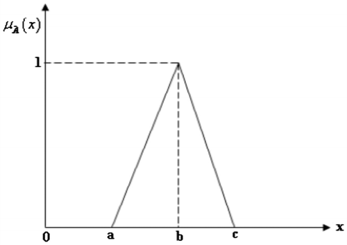
Triangular fuzzy numbers: A triangular fuzzy number can be defined as a triplet (a, b, c), where membership function can be defined as follows:(1) $${\mathit{\mu }}_{\tilde{A}}(x)=\left\{\begin{array}{cc}0,\hfill & x<a\hfill \\ \frac{x-a}{b-a},\hfill & a\le x\le b\hfill \\ \frac{c-x}{c-b},\hfill & b\le x\le c\hfill \\ 0,\hfill & c<x\hfill \end{array}\right.$$(1)

Graphically triangular fuzzy number is given in Figure 1.

2.2. The fuzzy arithmetic operations under function principle

Chen (1985) introduced function principle to define fuzzy arithmetical operations. We use this principle as the operations addition, multiplication, subtraction and division of triangular fuzzy numbers; because calculation as per function principle is easier than extension principle (Dubois & Prade, 1980) and does not change shape of triangular fuzzy number after applying operations.

Suppose $\tilde{A}=(a_1,a_2,a_3)$ and $\tilde{B}=(b_1,b_2,b_3)$ are triangular fuzzy numbers. Then,

(1)	The addition of $\tilde{A}$ and $\tilde{B}$ is $\tilde{A}\oplus \tilde{B}=(a_1+b_1,a_2+b_2,a_3+b_3)$, where a1, a2, a3, b1, b2, b3 are any real numbers.
(2)	The multiplication of $\tilde{A}$ and $\tilde{B}$ is $\tilde{A}\otimes \tilde{B}=(c_1,c_2,c_3)$, where $c_1=min\left\{a_1{b}_1,a_1{b}_3,a_3{b}_1,a_3{b}_3\right\}$, $c_2=a_2{b}_2$ and $c_3=max\left\{a_1{b}_1,a_1{b}_3,a_3{b}_1,a_3{b}_3\right\}$. i.e. $\tilde{A}\otimes \tilde{B}=(a_1{b}_1,a_2{b}_2,a_3{b}_3)$ with $a_1,a_2,a_3,b_1,b_2,b_3\in [0,1]$ are any real numbers.
(3)	Negative of $\tilde{B}$ defined as $-\tilde{B}=(-b_3,-b_2,-b_1)$, which defines subtraction of $\tilde{A}$ and $\tilde{B}$ as $\tilde{A}\sout{◯}\tilde{B}=(a_1-b_3,a_2-b_2,a_3-b_1)$.
(4)	Inverse of $\tilde{B}$ defined as $1/\tilde{B}=(1/b_3,1/b_2,1/b_1)$, which defines division of $\tilde{A}$ and $\tilde{B}$ is $\tilde{A}\mathrm{\varnothing }\tilde{B}=\left(a_1/b_3,a_2/b_2,a_3/b_1\right)$.
(5)	For any α ∊ R, then $\mathit{\alpha }\otimes \tilde{A}=(\mathit{\alpha }{a}_1,\mathit{\alpha }{a}_2,\mathit{\alpha }{a}_3)$ when α ≥ 0. Also, $\mathit{\alpha }\otimes \tilde{A}=(\mathit{\alpha }{a}_3,\mathit{\alpha }{a}_2,\mathit{\alpha }{a}_1)$ when α < 0.

2.3. Graded mean representation of a triangular fuzzy number

Given a triangular fuzzy number $\tilde{A}=(a_1,a_2,a_3)$, the graded mean representation of a triangular fuzzy number $\tilde{A}$ is defined as (Chou, 2003):(2) $$P(\tilde{A})=\frac{1}{6}(a_1+4a_2+a_3)$$(2)

Note that, a graded mean representation follows linearity property.

3. Mathematical model

In order to derive FEOP, we use following variables in formulation.

D	=	constant rate of demand
$\tilde{A}$	=	fuzzy ordering cost per order
$\tilde{h}$	=	fuzzy inventory holding cost per unit per time unit
${\tilde{C}}_p$	=	fuzzy purchase cost per unit
${\tilde{C}}_d$	=	fuzzy deterioration cost per unit deteriorated
T	=	total cycle time
Q	=	crisp ordering quantity

We assume that, inventory system deals with a single item, shortages are not allowed, replenishment rate is infinite, lead time zero and negligible, planning horizon is infinite and inventory deteriorates with rate of deterioration $\mathit{\theta }(t)=\frac{1}{1+m-t};0<t\le m$, where m is maximum lifetime. Here we take $\tilde{m}$ as fuzzy maximum lifetime as in most of the cases it is uncertain.

Remark

If t = m then item deteriorates completely as $\mathit{\theta }(t)=1$. Also consider either T < m or m ≤ T. Here, T < m shows item will deteriorate completely after cycle time, i.e. it can be used to satisfy demand up to cycle time with increasing rate of deterioration. But in case of m ≤ T inventory deteriorates completely before or up to cycle time. This case needs more importance while setting up cycle time.

First we formulate crisp model, by assuming all cost variables and maximum lifetime are crisp. Then we derive fuzzy formulation with relaxation that all cost variables and maximum lifetime as triangular fuzzy numbers.

3.1. Crisp model

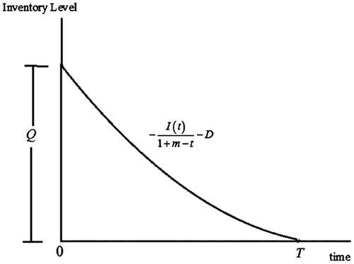
The flow of an inventory in inventory system is expressed in Figure 2. At time t = 0 stock is maximum and is same as Q (EOQ). Depletion in level of stock is cumulative effect of demand and deterioration of units.

Figure 2. Level of stock with respect to time.

Rate of change of level of stock in inventory system is managed by differential Equation (3),(3) $$\frac{\text{d}I(t)}{\text{dt}}+\frac{I(t)}{1+m-t}+D=0;0\le t\le T\text{where},I(0)=Q\text{and}I(T)=0$$(3)

Using boundary condition, solution of above differential equation is,(4) $$I(t)=D·\left(ln(1+m-t)-ln(1+m-T)\right)·(1+m-t);0\le t\le T$$(4)

Hence, EOQ is(5) $$Q=D·\left(ln(1+m)-ln(1+m-T)\right)·\left(1+m\right)$$(5)

The number of units deteriorated during cycle time is,(6) $$D_T={\int }_0^T\mathit{\theta }(t)I(t)\text{d}t$$(6)

Total amount of stock H_T present during cycle time is,(7) $$H_T={\int }_0^{T}I(t)\text{d}t$$(7)

Hence, the total average cost of an inventory system is defined as follows:(8) $$TC=\frac{1}{T}\left(OC+IHC+PC+DC\right)=\frac{1}{T}\left(A+h·H_T+C_p·Q+C_d·D_T\right)=\frac{1}{T}\left[\begin{array}{c}A+h(\frac{1}{2}Dln\left(1+m\right)m^2+Dln\left(1+m\right)m+\frac{1}{2}Dln\left(1+m\right)\hfill \\ -\frac{1}{2}Dln\left(1+m-T\right)m^2-Dln\left(1+m-T\right)m-\frac{1}{2}Dln\left(1+m-T\right)\hfill \\ +\frac{1}{4}D{T}^2-\frac{1}{2}DmT-\frac{1}{2}DT)+C_p\left(D·\left(ln\left(1+m\right)-ln\left(1+m-T\right)\right)·\left(1+m\right)\right)\hfill \\ +C_d\left(Dln\left(1+m\right)m+Dln\left(1+m\right)-DT-Dln\left(1+m-T\right)m-Dln\left(1+m-T\right)\right)\hfill \end{array}\right]$$(8)

3.2. Fuzzy model

Let us assume $\tilde{A}=\left(A_1,A_2,A_3\right)$, $\tilde{h}=(h_1,h_2,h_3)$, ${\tilde{C}}_p=\left(C_{p1},C_{p2},C_{p3}\right)$, ${\tilde{C}}_d=\left(C_{d1},C_{d2},C_{d3}\right)$ and $\tilde{m}=(m_1,m_2,m_3)$ are non negative triangular fuzzy numbers. Then we solve the optimal fuzzy total cost of an inventory system as $\tilde{T}C=\left(T{C}_1,T{C}_2,T{C}_3\right)$, where TC_i for i = 1, 2, 3 is defined as follows:(9) $$T{C}_i=\frac{1}{T}\left[\begin{array}{c}{A}_i+h_i\left(\frac{1}{2}Dln\left(1+m_i\right)m_i^2+Dln\left(1+m_i\right)m_i+\frac{1}{2}Dln\left(1+m_i\right)\right.\hfill \\ -\frac{1}{2}Dln\left(1+m_{4-i}-T\right)m_{4-i}^2-Dln\left(1+m_{4-i}-T\right)m_{4-i}\hfill \\ \left.-\frac{1}{2}Dln\left(1+m_{4-i}-T\right)+\frac{1}{4}D{T}^2-\frac{1}{2}D{m}_{4-i}T-\frac{1}{2}DT\right)\hfill \\ +C_{pi}\left(D·\left(ln\left(1+m_i\right)-ln\left(1+m_{4-i}-T\right)\right)·\left(1+m_{4-i}\right)\right)\hfill \\ +C_{di}\left(\begin{array}{c}Dln\left(1+m_i\right)m_i+Dln\left(1+m_i\right)-DT\hfill \\ -Dln\left(1+m_{4-i}-T\right)m_{4-i}-Dln\left(1+m_{4-i}-T\right)\hfill \end{array}\right)\hfill \end{array}\right]$$(9)

Secondly, we defuzzify the Fuzzy Total Inventory Cost (FTIC) using Graded Mean Representation Method. The result is,(10) $$P\left(\tilde{T}C\right)=\frac{1}{6}\left(T{C}_1+4T{C}_2+T{C}_3\right)$$(10)

Here, $P\left(\tilde{T}C\right)$ is a function of cycle time T. The optimal value of T (say T^*) is obtained by solving $\frac{dP\left(\tilde{T}C\right)}{dT}=0$ and used to find optimal value of FTCIS and EOQ Q, where $Q=\frac{1}{6}\left(Q_1+4Q_2+Q_3\right)$

with(11) $$Q_i=D·\left(ln(1+m_i)-ln(1+m_{4-i}-T)\right)·(1+m_i);i=1,2,3$$(11)

4. Numerical example and sensitivity analysis

To validate above mathematical formulation we consider example as follows. Costs are defined in $ and time is defined in

Figure 3. FTIC with respect to cycle time.

years.

Example

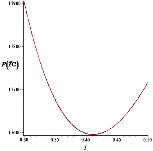
We take $\tilde{A}=(90,105,110)$, $\tilde{h}=(5,6,8)$, $\tilde{m}=(1.9,2.0,2.2)$, ${\tilde{C}}_p=(10,12,14)$, ${\tilde{C}}_d=(5,6,7)$ and D = 1,000. The optimal cycle time $T^{\ast }=0.412$ years and using this $Q^{\ast }=448.18$ units and $P\left(\tilde{T}C\right)=17595.09$. Graphical relationship between FTIC with respect to cycle time T is shown in Figure 3, and convexity validates optimality.

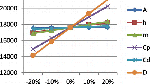
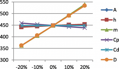
Sensitivity analysis is carried out by having variations in different parameters and exhibited in Tables 1–6.

Table 1. Variation with respect to $\tilde{A}$

$\tilde{A}$ (%)	T	$P\left(\tilde{T}C\right)$	Q
−20	0.408236	17,544.67	444.3508
−10	0.409894	17,569.93	446.272
0	0.411543	17,595.09	448.1847
10	0.413183	17,620.15	450.0891
20	0.414816	17,645.11	451.9853

Table 2. Variation with respect to $\tilde{h}$

$\tilde{h}$	T	$P\left(\tilde{T}C\right)$	Q
−20%	0.405847	16,968.64	441.5831
−10%	0.408849	17,282.01	445.0606
(5, 6, 8)	0.411543	17,595.09	448.1847
10%	0.413974	17,907.93	451.0073
20%	0.41618	18,220.56	453.5701

Table 3. Variation with respect to $\tilde{m}$

$\tilde{m}$	T	$P\left(\tilde{T}C\right)$	Q
−20%	0.334507	16,867.24	362.1256
−10%	0.372485	17,229.22	404.4898
(1.9, 2.0, 2.2)	0.411543	17,595.09	448.1847
10%	0.451581	17,964.34	493.0992
20%	0.492518	18,336.55	539.1367

Table 4. Variation with respect to ${\tilde{C}}_p$

${\tilde{C}}_p$	T	$P\left(\tilde{T}C\right)$	Q
−20%	0.420657	14,944.05	458.7791
−10%	0.415965	16,269.94	453.3207
(10, 12, 14)	0.411543	17,595.09	448.1847
10%	0.407366	18,919.56	443.3422
20%	0.403414	20,243.39	438.7676

Table 5. Variation with respect to ${\tilde{C}}_d$

${\tilde{C}}_d$	T	$P\left(\tilde{T}C\right)$	Q
−20%	0.411345	17,401.8	447.9556
−10%	0.411446	17,498.45	448.0722
(5, 6, 7)	0.411543	17,595.09	448.1847
10%	0.411636	17,691.74	448.2933
20%	0.411727	17,788.38	448.3982

Table 6. Variation with respect to D

D	T	$P\left(\tilde{T}C\right)$	Q
−20%	0.415629	14,126.04	362.3442
−10%	0.413365	15,860.64	405.2702
1,000	0.411543	17,595.09	448.1847
10%	0.410044	19,329.45	491.0908
20%	0.40879	21,063.73	533.9906

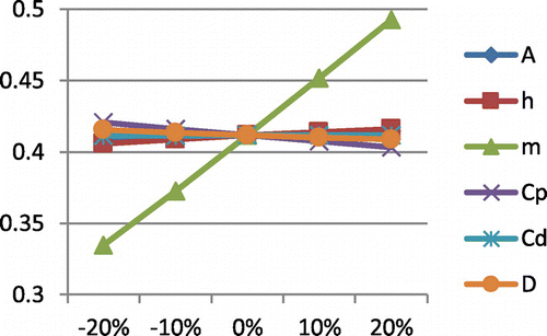
From Tables 1 to 6, one may observe that investment increase with respect to increment in all variables for which sensitivity is carried out. Cycle time is increased with respect to increase in ordering cost, holding cost, maximum lifetime of an item and cost due to deterioration, otherwise it decreases. EOQ is decreased with respect to increase in purchase cost only, otherwise it increases. One may observe these facts in Figures 4–6.

Figure 4. Variations in cycle time.

Figure 5. Variations in FTIC.

Figure 6. Variations in EOQ.

5. Conclusion

In this article, an FEOP is formulated to incorporate uncertainty in values of some variables like cost variables and importantly maximum lifetime of a product. Policy is formulated for a single item with constant rate of demand and deterioration rate depending upon maximum lifetime of an item. Formulation is supported with a numerical example and sensitivity is carried out for different parameters. Using tabular and graphical representation of sensitivity analysis, one may consider managerial insights discussed above. This paper provides interesting area for further study of inventory models with uncertain values of variable. One may consider problems of perfect or imperfect production system for future research.

Acknowledgement

The authors are very thankful to reviewers for their valuable comments to improve quality of this article. Also, they are thankful to editor for his continuous and caring support.

Additional information

Funding

Funding. The authors received no direct funding for this research.

Notes on contributors

Kunal T. Shukla

Kunal T. Shukla is the author of this manuscript and noteworthy efforts were made by Mihir S. Suthar in mathematical derivation of this article. Shukla is working as an assistant professor at Lukhdhirji Engineering College, Morbi, Gujarat, India. He has experience of teaching 11 years and research 4 years. His area of interest for research includes Supply Chain Management, Fuzzy Sets, Computational Mathematics.

References

- Aggarwal, S. P. (1978). A note on an order-level inventory model for a system with constant rate of deterioration. Operational Research, 15, 184–187.
- Bakker, M., Riezebos, J., & Teunter, R. H. (2012). Review of inventory systems with deterioration since 2001. European Journal of Operational Research, 221, 275–284.10.1016/j.ejor.2012.03.004
- Bhunia, A. K., & Maiti, M. (1999). An inventory model of deteriorating items with lot-size dependent replenishment cost and a linear trend in demand. Applied Mathematical Modelling, 23, 301–308.10.1016/S0307-904X(98)10089-6
- Chang, C. T., Ouyang, L.-Y., & Teng, J.-T. (2003). An EOQ model for deteriorating items under supplier credits linked to ordering quantity. Applied Mathematical Modelling, 27, 983–996.10.1016/S0307-904X(03)00131-8
- Chang, S.-C. (1999). Fuzzy production inventory for fuzzy product quantity with triangular fuzzy number. Fuzzy Sets and Systems, 107, 37–57.10.1016/S0165-0114(97)00350-3
- Chen, S. C., & Teng, J. T. (2013). Retailer’s optimal ordering policy for deteriorating items with maximum lifetime under supplier’s trade credit financing. Applied Mathematical Modeling, 38, 15–16.
- Chen, S. H. (1985). Operations on fuzzy numbers with function principle. Tamkang Journal of Management Science, 6, 13–27.
- Chen, S. H., & Hsieh, C. H. (2000). Optimization of fuzzy production inventory model under fuzzy parameters. In The Fifth Joint Conference on Information Sciences (JCIS2000) (Vol. 1, pp. 68–71). Atlantic City, NJ.
- Chou, C. C. (2003). The canonical representation of multiplication operation on triangular fuzzy numbers. Computers and Mathematics with Applications, 45, 1601–1610.10.1016/S0898-1221(03)00139-1
- Dubois, D., & Prade, H. (1980). Fuzzy sets and systems: Theory and applications (p. 26). New York, NY: Academic Press.
- Dye, C. Y., Hsieh, T. P., & Ouyang, L. Y. (2007). Determining optimal selling price and lot size with a varying rate of deterioration and exponential partial backlogging. European Journal of Operational Research, 181, 668–678.10.1016/j.ejor.2006.06.029
- Ghare, P. M., & Schrader, G. P. (1963). A model for an exponentially decaying inventory. Journal of Industrial Engineering, 14, 238–243.
- Goyal, S. K., & Giri, B. C. (2001). Recent trends in modeling of deteriorating inventory. European Journal of Operational Research, 134(1), 1–16.10.1016/S0377-2217(00)00248-4
- Hsieh, C. H. (2002). Optimization of fuzzy production inventory models. Information Sciences, 146, 29–40.10.1016/S0020-0255(02)00212-8
- Lee, H. M., & Yao, J. S. (1998). Economic production quantity for fuzzy demand quantity and fuzzy production quantity. European Journal of Operational Research, 109, 203–211.10.1016/S0377-2217(97)00200-2
- Nahmias, S. (1982). Perishable inventory theory: A review. Operations Research, 23, 735–749.
- Ouyang, L. Y., Wu, K. S., & Cheng, M. C. (2005). An inventory model for deteriorating items with exponential declining demand and partial backlogging. Yugoslav Journal of Operations Research, 15, 277–288.10.2298/YJOR0502277O
- Park, K. S. (1987). Fuzzy set theoretic interpretation of economic order quantity. IEEE Transactions on Systems, Man, and Cybernetics, 17, 1082–1084.10.1109/TSMC.1987.6499320
- Raafat, F. (1991). Survey of literature on continuously deteriorating inventory models. Journal of the Operational Research Society, 42, 27–37.10.1057/jors.1991.4
- Shah, N. H., Patel, D. G., & Shah, D. B. (2014). Optimal policies for deteriorating items with maximum lifetime and two-level trade credit. International Journal of Mathematics and Mathematical Sciences, 2014, 365929, 5 pp.
- Shah, N. H., & Shah, Y. K. (2000). Literature survey on inventory models for deteriorating items. Ekonomski anali, 44, 221–237.
- Shukla, K. T., & Suthar, M. S. (2016). A frame work for an inventory model for deterioration items with expiration under trapezoidal – type demand and partial backlogging. Logforum, 12, 269–281.
- Wang, W. C., Teng, J. T., & Lou, K. R. (2014). Seller’s optimal credit period and cycle time in a supply chain for deteriorating items with maximum lifetime. European Journal of Operational Research, 232, 315–321.10.1016/j.ejor.2013.06.027
- Wee, H. M. (1995). A deterministic lot size inventory model for deteriorating items with shortages and a declining market. Computer and Operation Research, 22, 345–356.
- Whitin, T. M. (1957). Theory of inventory management (pp. 62–72). Princeton, NJ: Princeton University Press.
- Yang, P. C., & Wee, H. M. (2003). An integrated multi-lot-size production inventory model for deteriorating item. Computers & Operations Research, 30, 671–682.10.1016/S0305-0548(02)00032-1