The generalized weighted Lindley distribution: Properties, estimation, and applications

Abstract

In this study, a three-parameter lifetime distribution namely generalized weighted Lindley (GLW) distribution is proposed. The GLW distribution is an useful generalization of the weighted Lindley distribution which accommodates increasing, decreasing, decreasing-increasing-decreasing, bathtub, and unimodal hazard rate making it a flexible model for reliable data. A significant account of mathematical properties for this distribution is presented. Different estimation procedures are discussed such as maximum likelihood estimators, method of moments, ordinary and weighted least-squares, percentile, maximum product of spacings, and minimum distance estimators. The estimators are compared by extensive numerical simulations. Finally, two data-sets are analyzed for illustrative purposes proving that the GWL outperforms several other three-parameter lifetime distributions.

Keywords:

• generalized weighted Lindley distribution
• Dierent estimation methods
• maximum product of spacings

Public Interest Statement

We have proposed and presented a probability distribution called generalized weighted Lindley (WL) distribution. This distribution is an useful generalization of the WL distribution which accommodates increasing, decreasing, decreasing-increasing-decreasing, bathtub, and unimodal hazard rate. A significant account of mathematical properties for this distribution was presented. Different estimation procedures were proposed and compared by extensive numerical simulations. We believe that new distribution will allow the users to describe different data-sets obtaining a better predictive performance in comparison with other usual distributions.

1. Introduction

In recent years, several new extensions of the exponential distribution have been introduced in the literature for describing real problems. Ghitany, Atieh, and Nadarajah (2008) investigated different properties of the Lindley distribution and outlined that in many cases the Lindley distribution outperforms exponential distribution. Since then, many generalizations of the Lindley distribution have been introduced such as generalized Lindley (Zakerzadeh & Dolati, 2009), extended Lindley (Bakouch, Al-Zahrani, Al-Shomrani, Marchi, & Louzada, 2012), exponential Poisson Lindley (Barreto-Souza & Bakouch, 2013), and Power Lindley (Ghitany, Al-Mutairi, Balakrishnan, & Al-Enezi, 2013) distribution.

Ghitany, Alqallaf, Al-Mutairi, and Husain (2011) introduced a new class of weighted Lindley (WL) distribution adding more flexibility to the Lindley distribution. Let T be a random variable with a WL distribution. Then probability density function (p.d.f) is given by(1) $$\begin{array}{c}\hfill f(t|\mathit{\lambda },\mathit{\varphi })=\frac{{\mathit{\lambda }}^{\mathit{\varphi }+1}}{(\mathit{\lambda }+\mathit{\varphi })\mathrm{\Gamma }(\mathit{\varphi })}{t}^{\mathit{\varphi }-1}(1+t)e^{-\mathit{\lambda }t},\end{array}$$(1)

for all $t>0$ , $\mathit{\varphi }>0$ and $\mathit{\lambda }>0$ and $\mathrm{\Gamma }(\mathit{\varphi })={\int }_0^{\infty }{e}^{-x}{x}^{\mathit{\varphi }-1}\text{d}x$ is the gamma function. One of its peculiarities is that the hazard function can have an increasing $(\mathit{\varphi }\ge 1)$ or bathtub $(0<\mathit{\varphi }<1)$ shape. Different properties and estimation methods for this model were presented by Mazucheli, Louzada, and Ghitany (2013), Ali (2015), Wang and Wang (in press), Al-Mutairi, Ghitany, and Kundu (2015).

In this study, a new lifetime distribution family is proposed which is a direct generalization of the WL distribution. The p.d.f is given by(2) $$\begin{array}{c}\hfill f(t|\mathit{\varphi },\mathit{\lambda },\mathit{\alpha })=\frac{\mathit{\alpha }{\mathit{\lambda }}^{\mathit{\alpha }\mathit{\varphi }}}{(\mathit{\lambda }+\mathit{\varphi })\mathrm{\Gamma }(\mathit{\varphi })}{t}^{\mathit{\alpha }\mathit{\varphi }-1}(\mathit{\lambda }+{(\mathit{\lambda }t)}^{\mathit{\alpha }})e^{-{(\mathit{\lambda }t)}^{\mathit{\alpha }}},\end{array}$$(2)

for all $t>0$, $\mathit{\varphi }>0,\mathit{\lambda }>0$ and $\mathit{\alpha }>0$. Important probability distributions can be obtained from the GWL distribution as the WL distribution ($\mathit{\alpha }=1$) , Power Lindley distribution ($\mathit{\varphi }=1$) and the Lindley distribution ($\mathit{\varphi }=1$ and $\mathit{\alpha }=1$). Due to this relationship, such model could also be named as weighted power Lindley or generalized power Lindley distribution.

Torabi, Falahati-Naeini, and Montazeri (2014) discussed a class of distribution with four parameters which is a generalization of the proposed model. Such distribution includes the generalized WL, generalized gamma (GG) distribution, gamma and Weibull, among others. The main difference of this study lies in the fact that the proposed three-parameter distribution has a simple structure with less computational issues. In this way, the behavior of the p.d.f and the hazard function can be studied. This model has different forms of hazard function such as increasing, decreasing, bathtub, unimodal, or decreasing-increasing-decreasing shape making the GWL distribution a flexible model for reliable data. Moreover, a significant account of mathematical properties for the new distribution is provided.

The inferential procedures for the parameters of GLW distribution are presented considering different methods such as maximum likelihood estimators (MLE), methods of moments (ME), ordinary least-squares estimation (OLSE), weighted least-squares estimation (WLSE), maximum product of spacings (MPS), Cramer-von Mises type minimum distance (CME), Anderson–Darling (ADE) and right-tail Anderson–Darling (RADE). The performance of these estimation procedures are compared using extensive numerical simulations. Finally, two data-sets are analyzed for illustrative purposes proving that the GWL outperforms several usual three-parameter lifetime distributions such as the GG distribution (Stacy, 1962), the generalized Weibull (GW) distribution (Mudholkar, Srivastava, & Kollia, 1996), the generalized exponential-Poisson (GEP) distribution (Barreto-Souza & Cribari-Neto, 2009), and the exponentiated Weibull (EW) distribution (Mudholkar, Srivastava, & Freimer, 1995).

The results of this paper are organized as follows. Section 2 provides a significant account of mathematical properties for the new distribution. Section 3 presents the eight estimation methods which are considered. In the Section 4, a simulation study is presented in order to identify the most efficient procedure. Section 5 illustrates the proposed methodology in two real data-sets. Section 6 summarizes the present work.

2. Generalized weighted Lindley distribution

The generalized WL distribution (2) can be expressed as a two-component mixture$$\begin{array}{c}\hfill f(t|\mathit{\varphi },\mathit{\lambda },\mathit{\alpha })=p{f}_1(t|\mathit{\varphi },\mathit{\lambda },\mathit{\alpha })+(1-p)f_2(t|\mathit{\varphi },\mathit{\lambda },\mathit{\alpha })\end{array}$$

where $p=\mathit{\lambda }/(\mathit{\lambda }+\mathit{\varphi })$ and $T_j\sim \text{GG}(\mathit{\varphi }+j-1,\mathit{\lambda },\mathit{\alpha })$, for $j=1,2$, i.e. $f_j(t|\mathit{\lambda },\mathit{\varphi })$ has GG distribution, given by(3) $$\begin{array}{c}\hfill f_j(t|\mathit{\varphi },\mathit{\lambda },\mathit{\alpha })=\frac{\mathit{\alpha }}{\mathrm{\Gamma }(\mathit{\varphi }+j-1)}{\mathit{\lambda }}^{\mathit{\alpha }(\mathit{\varphi }+j-1)}{t}^{\mathit{\alpha }(\mathit{\varphi }+j-1)-1}{e}^{-{(\mathit{\lambda }t)}^{\mathit{\alpha }}}.\end{array}$$(3)

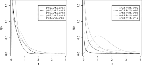
The behavior of the p.d.f. (2) when $t\to 0$ and $t\to \infty$ are, respectively, given by$$\begin{array}{c}\hfill f(0)=\left\{\begin{array}{cc}\infty ,\hfill & \text{if}\mathit{\alpha }\mathit{\varphi }<1\hfill \\ {\displaystyle \frac{\mathit{\alpha }{\mathit{\lambda }}^2}{(\mathit{\lambda }+\mathit{\varphi })\mathrm{\Gamma }(\mathit{\varphi })}},\hfill & \text{if}\mathit{\alpha }\mathit{\varphi }=1\hfill \\ 0,\hfill & \text{if}\mathit{\alpha }\mathit{\varphi }>1\hfill \end{array}\right.,f(\infty )=0.\end{array}$$

Figure 1 gives examples of the shapes of the density function for different values of $\mathit{\varphi },\mathit{\lambda }$ and $\mathit{\alpha }$.

Figure 1. Density function shapes for GWL distribution considering different values of $\mathit{\varphi },\mathit{\lambda }$ and $\mathit{\alpha }$.

The cumulative distribution function from the GWL distribution is given by(4) $$\begin{array}{c}\hfill F(t|\mathit{\varphi },\mathit{\lambda },\mathit{\alpha })=\frac{\mathit{\gamma }\left[\mathit{\varphi },{(\mathit{\lambda }t)}^{\mathit{\alpha }}\right](\mathit{\lambda }+\mathit{\varphi })-{(\mathit{\lambda }t)}^{\mathit{\alpha }\mathit{\varphi }}{e}^{-{(\mathit{\lambda }t)}^{\mathit{\alpha }}}}{(\mathit{\lambda }+\mathit{\varphi })\mathrm{\Gamma }(\mathit{\varphi })}\end{array}$$(4)

where $\mathit{\gamma }[y,x]={\int }_0^x{w}^{y-1}{e}^{-w}\text{d}w$ is the lower incomplete gamma function.

2.1. Moments

Many important features and properties of a distribution can be obtained through its moments such as mean, variance, kurtosis, and skewness. In this section, important moment functions such as the moment-generating function, r-th moment, r-th central moment, among others are presented.

Theorem 2.1

For the random variable T with GWL distribution, the moment-generating function is given by(5) $$\begin{array}{c}\hfill M_X(t)=\sum _{r=0}^{\infty }\frac{t^r}{{\mathit{\lambda }}^{r}r!}\frac{\left(\frac{r}{\mathit{\alpha }}+\mathit{\varphi }+\mathit{\lambda }\right)\mathrm{\Gamma }(\frac{r}{\mathit{\alpha }}+\mathit{\varphi })}{(\mathit{\lambda }+\mathit{\varphi })\mathrm{\Gamma }(\mathit{\varphi })}.\end{array}$$(5)

Proof

Note that, the moment-generating function from GG distribution (3) is given by$$\begin{array}{c}\hfill M_{X,j}(t)=\sum _{r=0}^{\infty }\frac{t^r}{r!}\frac{\mathrm{\Gamma }\left(\frac{r}{\mathit{\alpha }}+\mathit{\varphi }+j-1\right)}{{\mathit{\lambda }}^r\mathrm{\Gamma }(\mathit{\varphi }+j-1)}.\end{array}$$

Since the GWL distribution (2) can be expressed as a two-component mixture, we have$$\begin{array}{cc}\hfill M_X(t)& =E\left[e^{tX}\right]=\underset{0}{\overset{\infty }{\int }}{e}^{tx}f(x|\mathit{\varphi },\mathit{\lambda },\mathit{\alpha })\text{d}x=p{M}_{X,1}(t)+(1-p)M_{X,2}(t)\hfill \\ \hfill & =\frac{\mathit{\lambda }}{(\mathit{\lambda }+\mathit{\varphi })}\sum _{r=0}^{\infty }\frac{t^r}{r!}\frac{\mathrm{\Gamma }\left(\frac{r}{\mathit{\alpha }}+\mathit{\varphi }\right)}{{\mathit{\lambda }}^r\mathrm{\Gamma }(\mathit{\varphi })}+\frac{\mathit{\varphi }}{(\mathit{\lambda }+\mathit{\varphi })}\sum _{r=0}^{\infty }\frac{t^r}{r!}\frac{\mathrm{\Gamma }\left(\frac{r}{\mathit{\alpha }}+\mathit{\varphi }+1\right)}{{\mathit{\lambda }}^r\mathrm{\Gamma }(\mathit{\varphi }+1)}\hfill \\ \hfill & =\frac{1}{(\mathit{\lambda }+\mathit{\varphi })}\sum _{r=0}^{\infty }\frac{t^r}{r!}\frac{\mathit{\lambda }\mathrm{\Gamma }(\frac{r}{\mathit{\alpha }}+\mathit{\varphi })}{{\mathit{\lambda }}^r\mathrm{\Gamma }(\mathit{\varphi })}+\frac{1}{(\mathit{\lambda }+\mathit{\varphi })}\sum _{r=0}^{\infty }\frac{t^r}{r!}\frac{\left(\frac{r}{\mathit{\alpha }}+\mathit{\varphi }\right)\mathrm{\Gamma }\left(\frac{r}{\mathit{\alpha }}+\mathit{\varphi }\right)}{{\mathit{\lambda }}^r\mathrm{\Gamma }(\mathit{\varphi })}\hfill \\ \hfill & =\sum _{r=0}^{\infty }\frac{t^r}{{\mathit{\lambda }}^{r}r!}\frac{\left(\frac{r}{\mathit{\alpha }}+\mathit{\varphi }+\mathit{\lambda }\right)\mathrm{\Gamma }\left(\frac{r}{\mathit{\alpha }}+\mathit{\varphi }\right)}{(\mathit{\lambda }+\mathit{\varphi })\mathrm{\Gamma }(\mathit{\varphi })}.\hfill \end{array}$$$\square$

Corollary 2.2

For the random variable T with GWL distribution, the r-th moment is given by(6) $$\begin{array}{c}\hfill {\mathit{\mu }}_r=E[T^r]=\frac{\left(\frac{r}{\mathit{\alpha }}+\mathit{\varphi }+\mathit{\lambda }\right)\mathrm{\Gamma }\left(\frac{r}{\mathit{\alpha }}+\mathit{\varphi }\right)}{(\mathit{\lambda }+\mathit{\varphi }){\mathit{\lambda }}^r\mathrm{\Gamma }(\mathit{\varphi })}.\end{array}$$(6)

Proof

Note that, ${\mathit{\mu }}_r=M_X^{(r)}(0)=\frac{d^n{M}_X(0)}{\text{d}{t}^n}$ and the result follows. $\square$

Corollary 2.3

For the random variable T with GWL distribution, the r-th central moment is given by(7) $$\begin{array}{cc}\hfill M_r& =E{[T-\mathit{\mu }]}^r=\sum _{i=0}^r\left(\begin{array}{c}r\\ i\end{array}\right){(-\mathit{\mu })}^{r-i}E[T^i]\hfill \\ \hfill & =\sum _{i=0}^r\left(\begin{array}{c}r\\ i\end{array}\right){\left(-\frac{\left(\frac{1}{\mathit{\alpha }}+\mathit{\varphi }+\mathit{\lambda }\right)\mathrm{\Gamma }\left(\frac{1}{\mathit{\alpha }}+\mathit{\varphi }\right)}{\mathit{\lambda }(\mathit{\lambda }+\mathit{\varphi })\mathrm{\Gamma }(\mathit{\varphi })}\right)}^{r-i}\frac{\left(\frac{i}{\mathit{\alpha }}+\mathit{\varphi }+\mathit{\lambda }\right)\mathrm{\Gamma }(\frac{i}{\mathit{\alpha }}+\mathit{\varphi })}{(\mathit{\lambda }+\mathit{\varphi }){\mathit{\lambda }}^i\mathrm{\Gamma }(\mathit{\varphi })}.\hfill \end{array}$$(7)

Corollary 2.4

A random variable T with GWL distribution has the mean and variance respectively given by(8) $$\begin{array}{cc}\hfill \mathit{\mu }& =\frac{\left(\frac{1}{\mathit{\alpha }}+\mathit{\varphi }+\mathit{\lambda }\right)\mathrm{\Gamma }\left(\frac{1}{\mathit{\alpha }}+\mathit{\varphi }\right)}{\mathit{\lambda }(\mathit{\lambda }+\mathit{\varphi })\mathrm{\Gamma }(\mathit{\varphi })},\hfill \end{array}$$(8) (9) $$\begin{array}{cc}\hfill {\mathit{\sigma }}^2& =\frac{\mathit{\lambda }(\mathit{\lambda }+\mathit{\varphi })\left(\frac{2}{\mathit{\alpha }}+\mathit{\varphi }+\mathit{\lambda }\right)\mathrm{\Gamma }\left(\frac{2}{\mathit{\alpha }}+\mathit{\varphi }\right)-{\left(\frac{1}{\mathit{\alpha }}+\mathit{\varphi }+\mathit{\lambda }\right)}^2\mathrm{\Gamma }{\left(\frac{1}{\mathit{\alpha }}+\mathit{\varphi }\right)}^2}{{\mathit{\lambda }}^2{(\mathit{\lambda }+\mathit{\varphi })}^2\mathrm{\Gamma }{(\mathit{\varphi })}^2}.\hfill \end{array}$$(9)

Proof

From (6) and considering $r=1$ we have ${\mathit{\mu }}_1=\mathit{\mu }$. The second result follows from (7) considering $r=2$ with some algebraic manipulations. $\square$

Another moment function that can be easily achieved for GWL distribution and plays an important role in information theory is given by(10) $$\begin{array}{c}\hfill E[log(T)]=\frac{\left(\mathit{\psi }(\mathit{\varphi })-\mathit{\alpha }log\mathit{\lambda }+{(\mathit{\lambda }+\mathit{\varphi })}^{-1}\right)}{\mathit{\alpha }}.\end{array}$$(10)

2.2. Survival properties

In this section, we present the survival, hazard, and mean residual life (MRL) function for the GWL distribution. The survival function of T is given by(11) $$\begin{array}{c}\hfill S(t|\mathit{\varphi },\mathit{\lambda },\mathit{\alpha })=\frac{\mathrm{\Gamma }\left[\mathit{\varphi },{(\mathit{\lambda }t)}^{\mathit{\alpha }}\right](\mathit{\lambda }+\mathit{\varphi })+{(\mathit{\lambda }t)}^{\mathit{\alpha }\mathit{\varphi }}{e}^{-{(\mathit{\lambda }t)}^{\mathit{\alpha }}}}{(\mathit{\lambda }+\mathit{\varphi })\mathrm{\Gamma }(\mathit{\varphi })}\end{array}$$(11)

where $\mathrm{\Gamma }(x,y)={\int }_0^x{w}^{y-1}{e}^{-x}\text{d}w$ is called upper incomplete gamma. The hazard function is given as(12) $$\begin{array}{c}\hfill h(t|\mathit{\varphi },\mathit{\lambda },\mathit{\alpha })=\frac{f(t|\mathit{\varphi },\mathit{\lambda },\mathit{\alpha })}{S(t|\mathit{\varphi },\mathit{\lambda },\mathit{\alpha })}=\frac{\mathit{\alpha }{\mathit{\lambda }}^{\mathit{\alpha }\mathit{\varphi }}{t}^{\mathit{\alpha }\mathit{\varphi }-1}(\mathit{\lambda }+{(\mathit{\lambda }t)}^{\mathit{\alpha }})e^{-{(\mathit{\lambda }t)}^{\mathit{\alpha }}}}{\mathrm{\Gamma }\left[\mathit{\varphi },{(\mathit{\lambda }t)}^{\mathit{\alpha }}\right](\mathit{\lambda }+\mathit{\varphi })+{(\mathit{\lambda }t)}^{\mathit{\alpha }\mathit{\varphi }}{e}^{-{(\mathit{\lambda }t)}^{\mathit{\alpha }}}}.\end{array}$$(12)

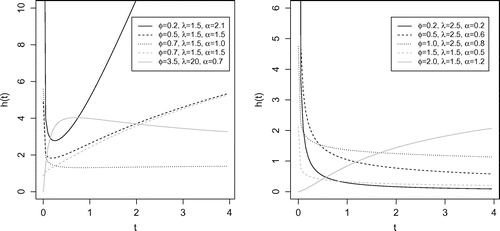
The behavior of the hazard function (12) when $t\to 0$ and $t\to \infty$ are, respectively, given by$$\begin{array}{c}\hfill h(0)=\left\{\begin{array}{cc}\infty ,\hfill & \text{if}\mathit{\alpha }\mathit{\varphi }<1\hfill \\ {\displaystyle \frac{\mathit{\alpha }{\mathit{\lambda }}^2}{(\mathit{\lambda }+\mathit{\varphi })\mathrm{\Gamma }(\mathit{\varphi })}},\hfill & \text{if}\mathit{\alpha }\mathit{\varphi }=1\hfill \\ 0,\hfill & \text{if}\mathit{\alpha }\mathit{\varphi }>1\hfill \end{array}\right.\text{and}h(\infty )=\left\{\begin{array}{cc}0,\hfill & \text{if}\mathit{\alpha }\mathit{\varphi }<1\hfill \\ \mathit{\lambda },\hfill & \text{if}\mathit{\alpha }\mathit{\varphi }=1\hfill \\ \infty ,\hfill & \text{if}\mathit{\alpha }\mathit{\varphi }>1.\hfill \end{array}\right.\end{array}$$

Theorem 2.5

The hazard rate function h(t) of the GWL distribution is increasing, decreasing, bathtub, unimodal, or decreasing-increasing-decreasing shaped.

Proof

The theorem proposed by Glaser (1980) is not easily applied in the GLW distribution. Since the hazard rate function (12) is complex, we considered the following cases:

(1)	Let $\mathit{\alpha }=1$, then GWL distribution reduces to the WL distribution. Ghitany et al. (2011) proved that the hazard function is bathtub-shaped (increasing) if $0<\mathit{\varphi }<1$$(\mathit{\varphi }>0)$, for all $\mathit{\lambda }>0$.
(2)	Let $\mathit{\varphi }=1$, then GWL distribution reduces to the PL distribution. Considering $\mathit{\beta }={\mathit{\lambda }}^{\mathit{\alpha }}$, Ghitany et al. (2013) proved that the hazard function is

 

• increasing when $\left\{0<\mathit{\alpha }\ge 1,\mathit{\beta }>0\right\}$;

• decreasing when $\left\{0<\mathit{\alpha }\le \frac{1}{2},\mathit{\beta }>0\right\}$ or $\left\{\frac{1}{2}<\mathit{\alpha }<1,\mathit{\beta }\ge {(2\mathit{\alpha }-1)}^2{(4\mathit{\alpha }(1-\mathit{\alpha }))}^{-1}\right\}$;

• decreasing-increasing-decreasing if $\left\{\frac{1}{2}<\mathit{\alpha }<1,0<\mathit{\beta }<{(2\mathit{\alpha }-1)}^2{(4\mathit{\alpha }(1-\mathit{\alpha }))}^{-1}\right\}$.

 

(3)	Let $\mathit{\alpha }=2$ and $\mathit{\lambda }=1$, from Glaser’s theorem (Glaser, 1980), the hazard rate function is decreasing shaped (unimodal) for $0<\mathit{\varphi }<1$$(\mathit{\varphi }>1)$.

$\square$

These properties make the GWL distribution a flexible model for reliable data. Figure 2 gives examples of the shapes of the hazard function for different values of $\mathit{\varphi },\mathit{\lambda }$ and $\mathit{\alpha }$.

Figure 2. Hazard function shapes for GWL distribution and considering different values of $\mathit{\varphi },\mathit{\lambda }$ and $\mathit{\alpha }$.

The MRL has been widely used in survival analysis and represents the expected additional lifetime given that a component has survived until time t.

Proposition 2.6

The MRL function $r(t|\mathit{\varphi },\mathit{\lambda },\mathit{\alpha })$ of the GWL distribution is given by(13) $$\begin{array}{c}\hfill r(t|\mathit{\varphi },\mathit{\lambda },\mathit{\alpha })=\frac{\left(\mathit{\varphi }+\frac{1}{\mathit{\alpha }}+\mathit{\lambda }\right)\mathrm{\Gamma }\left(\mathit{\varphi }+\frac{1}{\mathit{\alpha }},{\left(\mathit{\lambda }t\right)}^{\mathit{\alpha }}\right)-\mathit{\lambda }t(\mathit{\lambda }+\mathit{\varphi })\mathrm{\Gamma }\left(\mathit{\varphi },{\left(\mathit{\lambda }t\right)}^{\mathit{\alpha }}\right)}{\mathit{\lambda }[(\mathit{\lambda }+\mathit{\varphi })\mathrm{\Gamma }(\mathit{\varphi },{\left(\mathit{\lambda }t\right)}^{\mathit{\alpha }})+{(\mathit{\lambda }t)}^{\mathit{\alpha }\mathit{\varphi }}{e}^{-{\left(\mathit{\lambda }t\right)}^{\mathit{\alpha }}}]}.\end{array}$$(13)

Proof

Note that$$\begin{array}{cc}\hfill r(t|\mathit{\varphi },\mathit{\lambda },\mathit{\alpha })& =\frac{1}{S(t)}\underset{t}{\overset{\infty }{\int }}yf(y|\mathit{\lambda },\mathit{\varphi })\text{d}y-t\hfill \\ \hfill & =\frac{1}{S(t)}\left[p\underset{t}{\overset{\infty }{\int }}y{f}_1(y|\mathit{\lambda },\mathit{\varphi })\text{d}y+(1-p){\int }_x^{\infty }y{f}_2(y|\mathit{\lambda },\mathit{\varphi })\text{d}y\right]-t\hfill \\ \hfill & =\frac{\left(\mathit{\varphi }+\frac{1}{\mathit{\alpha }}+\mathit{\lambda }\right)\mathrm{\Gamma }\left(\mathit{\varphi }+\frac{1}{\mathit{\alpha }},{\left(\mathit{\lambda }t\right)}^{\mathit{\alpha }}\right)-\mathit{\lambda }t(\mathit{\lambda }+\mathit{\varphi })\mathrm{\Gamma }\left(\mathit{\varphi },{\left(\mathit{\lambda }t\right)}^{\mathit{\alpha }}\right)}{\mathit{\lambda }[(\mathit{\lambda }+\mathit{\varphi })\mathrm{\Gamma }(\mathit{\varphi },{\left(\mathit{\lambda }t\right)}^{\mathit{\alpha }})+{(\mathit{\lambda }t)}^{\mathit{\alpha }\mathit{\varphi }}{e}^{-{\left(\mathit{\lambda }t\right)}^{\mathit{\alpha }}}]}.\hfill \end{array}$$$\square$

The behavior of the MRL function when $t\to 0$ and $t\to \infty$ are, respectively, given by$$\begin{array}{c}\hfill r(0)=\frac{1}{\mathit{\lambda }\left((\mathit{\lambda }+\mathit{\varphi })\mathrm{\Gamma }(\mathit{\varphi })\right)}\text{and}r(\infty )\left\{\begin{array}{cc}\infty ,\hfill & \text{if}\mathit{\alpha }<1\hfill \\ {\displaystyle \frac{1}{\mathit{\lambda }}},\hfill & \text{if}\mathit{\alpha }=1\hfill \\ 0,\hfill & \text{if}\mathit{\alpha }>1.\hfill \end{array}\right.\end{array}$$

2.3. Entropy

In information theory, entropy has played a central role as a measure of uncertainty associated with a random variable. Shannon’s entropy is one of the most important metrics in information theory. For the GWL distribution, Shannon’s entropy can be obtained by solving(14) $$\begin{array}{c}\hfill H_S(\mathit{\varphi },\mathit{\lambda },\mathit{\alpha })=-\underset{0}{\overset{\infty }{\int }}log\left(\frac{\mathit{\alpha }{\mathit{\lambda }}^{\mathit{\alpha }\mathit{\varphi }}{t}^{\mathit{\alpha }\mathit{\varphi }-1}(\mathit{\lambda }+{(\mathit{\lambda }t)}^{\mathit{\alpha }})e^{-{(\mathit{\lambda }t)}^{\mathit{\alpha }}}}{(\mathit{\lambda }+\mathit{\varphi })\mathrm{\Gamma }(\mathit{\varphi })}\right)f(t|\mathit{\varphi },\mathit{\lambda },\mathit{\alpha })\text{d}t.\end{array}$$(14)

Proposition 2.7

A random variable T with GWL distribution has Shannon’s entropy given by(15) $$\begin{array}{cc}\hfill H_S(\mathit{\varphi },\mathit{\lambda },\mathit{\alpha })& =log(\mathit{\lambda }+\mathit{\varphi })+log\mathrm{\Gamma }(\mathit{\varphi })-log\mathit{\alpha }-log\mathit{\lambda }-\frac{\mathit{\varphi }(1+\mathit{\varphi }+\mathit{\lambda })}{(\mathit{\lambda }+\mathit{\varphi })}\hfill \\ \hfill & -\frac{\mathit{\psi }(\mathit{\varphi })(\mathit{\alpha }\mathit{\varphi }-1)}{\mathit{\alpha }}-\frac{(\mathit{\alpha }\mathit{\varphi }-1)}{\mathit{\alpha }(\mathit{\lambda }+\mathit{\varphi })}-\frac{\mathit{\eta }(\mathit{\varphi },\mathit{\lambda })}{(\mathit{\lambda }+\mathit{\varphi })\mathrm{\Gamma }(\mathit{\varphi })}\hfill \end{array}$$(15)

where$$\begin{array}{c}\hfill \mathit{\eta }(\mathit{\varphi },\mathit{\lambda })=\underset{0}{\overset{\infty }{\int }}(\mathit{\lambda }+y)log(\mathit{\lambda }+y)y^{\mathit{\varphi }-1}{e}^{-y}\text{d}y=\underset{0}{\overset{1}{\int }}(\mathit{\lambda }-logu)log(\mathit{\lambda }-logu){(-logu)}^{\mathit{\varphi }-1}\text{d}u.\end{array}$$

Proof

From the Equation (14), we have(16) $$\begin{array}{cc}\hfill H_S(\mathit{\varphi },\mathit{\lambda },\mathit{\alpha })& =-log\mathit{\alpha }-\mathit{\alpha }\mathit{\varphi }log\mathit{\lambda }+log(\mathit{\lambda }+\mathit{\varphi })+log(\mathrm{\Gamma }(\mathit{\varphi }))+{\mathit{\lambda }}^{\mathit{\alpha }}E[T^{\mathit{\alpha }}]\hfill \\ \hfill & -(\mathit{\alpha }\mathit{\varphi }-1)E[logT]-E\left[log(\mathit{\lambda }+{(\mathit{\lambda }T)}^{\mathit{\alpha }})\right].\hfill \end{array}$$(16)

Note that$$\begin{array}{c}\hfill E\left[log(\mathit{\lambda }+{(\mathit{\lambda }T)}^{\mathit{\alpha }})\right]=\underset{0}{\overset{\infty }{\int }}{log(\mathit{\lambda }+(\mathit{\lambda }T)}^{\mathit{\alpha }}\frac{\mathit{\alpha }{\mathit{\lambda }}^{\mathit{\alpha }\mathit{\varphi }}{t}^{\mathit{\alpha }\mathit{\varphi }-1}(\mathit{\lambda }+{(\mathit{\lambda }t)}^{\mathit{\alpha }})e^{-{(\mathit{\lambda }t)}^{\mathit{\alpha }}}}{(\mathit{\lambda }+\mathit{\varphi })\mathrm{\Gamma }(\mathit{\varphi })}\text{d}t,\end{array}$$

using the change of variable $y={(\mathit{\lambda }t)}^{\mathit{\alpha }}$ and after some algebra$$\begin{array}{cc}\hfill E\left[log(\mathit{\lambda }+{(\mathit{\lambda }T)}^{\mathit{\alpha }})\right]& =\frac{1}{(\mathit{\lambda }+\mathit{\varphi })\mathrm{\Gamma }(\mathit{\varphi })}\underset{0}{\overset{\infty }{\int }}(\mathit{\lambda }+y)log(\mathit{\lambda }+y)y^{\mathit{\varphi }-1}{e}^{-y}\text{d}y\hfill \\ \hfill & =\frac{\mathit{\eta }(\mathit{\varphi },\mathit{\lambda })}{(\mathit{\lambda }+\mathit{\varphi })\mathrm{\Gamma }(\mathit{\varphi })}.\hfill \end{array}$$

From Equations (6) and (10), we can easily find the solution of $E[T^{\mathit{\alpha }}]$ and $E[logT]$ and the result as follows. $\square$

Another popular entropy measure is proposed by Renyi (1961). Some recent applications of the Renyi entropy can be seen in Popescu and Aiordachioaie (2013). If T has the probability density function (1) then Renyi entropy is defined by(17) $$\begin{array}{c}\hfill \frac{1}{1-\mathit{\rho }}log\underset{0}{\overset{\infty }{\int }}{f}^{\mathit{\rho }}(x)\text{d}x.\end{array}$$(17)

Proposition 2.8

A random variable T with GWL distribution, has the Renyi entropy given by(18) $$\begin{array}{c}\hfill H_R(\mathit{\rho })=\frac{(\mathit{\rho }-1)(log\mathit{\alpha }+log\mathit{\lambda })-\mathit{\rho }\left(log(\mathit{\lambda }+\mathit{\varphi })+log\mathrm{\Gamma }(\mathit{\varphi })\right)-log(\mathit{\delta }(\mathit{\rho },\mathit{\varphi },\mathit{\lambda },\mathit{\alpha }))}{1-\mathit{\rho }}\end{array}$$(18)

where $\mathit{\delta }(\mathit{\rho },\mathit{\varphi },\mathit{\lambda },\mathit{\alpha })=\underset{0}{\overset{\infty }{\int }}{y}^{\frac{\mathit{\rho }\mathit{\varphi }-\mathit{\rho }+1-\mathit{\alpha }}{\mathit{\alpha }}}{(\mathit{\lambda }+y)}^{\mathit{\rho }}{e}^{-\mathit{\rho }y}\text{d}y$.

Proof

The Renyi entropy is given by$$\begin{array}{cc}\hfill H_R(\mathit{\rho })& =\frac{1}{1-\mathit{\rho }}log\left(\frac{{\mathit{\alpha }}^{\mathit{\rho }}{\mathit{\lambda }}^{\mathit{\rho }}}{{(\mathit{\lambda }+\mathit{\varphi })}^{\mathit{\rho }}\mathrm{\Gamma }{(\mathit{\varphi })}^{\mathit{\rho }}}\underset{0}{\overset{\infty }{\int }}{(\mathit{\lambda }t)}^{\mathit{\alpha }\mathit{\rho }\left(\mathit{\varphi }-\frac{1}{\mathit{\alpha }}\right)}{\left(\mathit{\lambda }+{(\mathit{\lambda }t)}^{\mathit{\alpha }}\right)}^{\mathit{\rho }}{e}^{-\mathit{\rho }{(\mathit{\lambda }t)}^{\mathit{\alpha }}}\text{d}t\right)\hfill \\ \hfill & =\frac{1}{1-\mathit{\rho }}log\left(\frac{{\mathit{\alpha }}^{\mathit{\rho }}{\mathit{\lambda }}^{\mathit{\rho }}}{{(\mathit{\lambda }+\mathit{\varphi })}^{\mathit{\rho }}\mathrm{\Gamma }{(\mathit{\varphi })}^{\mathit{\rho }}}\underset{0}{\overset{\infty }{\int }}{y}^{\frac{\mathit{\rho }\mathit{\varphi }-\mathit{\rho }+1-\mathit{\alpha }}{\mathit{\alpha }}}{(\mathit{\lambda }+y)}^{\mathit{\rho }}{e}^{-\mathit{\rho }y}\text{d}y\right)\hfill \\ \hfill & =\frac{1}{1-\mathit{\rho }}log\left(\frac{{\mathit{\alpha }}^{\mathit{\rho }}{\mathit{\lambda }}^{\mathit{\rho }}}{{(\mathit{\lambda }+\mathit{\varphi })}^{\mathit{\rho }}\mathrm{\Gamma }{(\mathit{\varphi })}^{\mathit{\rho }}}\mathit{\delta }(\mathit{\rho },\mathit{\varphi },\mathit{\lambda },\mathit{\alpha })\right)\hfill \end{array}$$

and with some algebra the proof is completed. $\square$

2.4. Lorenz curves

The Lorenz curve (Bonferroni, 1930) is a well-known measure used in reliability, income inequality, life testing and renewal theory. The Lorenz curve for a non-negative T random variable is given through the consecutive plot of$$\begin{array}{c}\hfill L\left(F(t)\right)=\frac{\underset{0}{\overset{t}{\int }}xf(x)\text{d}x}{\underset{0}{\overset{\infty }{\int }}xf(x)\text{d}x}=\frac{1}{\mathit{\mu }}{\int }_0^{t}xf(x)\text{d}x.\end{array}$$

Proposition 2.9

The Lorenz curve for the GWL distribution is$$\begin{array}{c}\hfill L\left(p\right)=\frac{\left(\frac{1}{\mathit{\alpha }}+\mathit{\varphi }+\mathit{\lambda }\right)\mathit{\gamma }\left(\mathit{\varphi }+\frac{1}{\mathit{\alpha }},{\left(\mathit{\lambda }{F}^{-1}(p)\right)}^{\mathit{\alpha }}\right)-{\left(\mathit{\lambda }{F}^{-1}(p)\right)}^{\mathit{\alpha }\mathit{\varphi }-1}{e}^{-{\left(\mathit{\lambda }{F}^{-1}(p)\right)}^{\mathit{\alpha }}}}{\left(\frac{1}{\mathit{\alpha }}+\mathit{\varphi }+\mathit{\lambda }\right)\mathrm{\Gamma }\left[\frac{1}{\mathit{\alpha }}+\mathit{\varphi }\right]}\end{array}$$

where $F^{-1}(p)=t_p$.

3. Methods of estimation

In this section, we present eight different estimation methods for the parameters $\mathit{\varphi },\mathit{\lambda }$ and $\mathit{\alpha }$ of the GWL distribution.

3.1. Maximum likelihood estimation

The maximum likelihood method has been widely used due to its better asymptotic properties. The estimates are obtained by maximizing the likelihood function. Let $T_1,\dots ,T_n$ be a random sample where $T\sim \text{GWL}(\mathit{\varphi },\mathit{\lambda },\mathit{\alpha })$, the likelihood function is given by(19) $$\begin{array}{c}\hfill L(\mathit{\varphi },\mathit{\lambda },\mathit{\alpha };\mathit{t})=\frac{{\mathit{\alpha }}^n{\mathit{\lambda }}^{n\mathit{\alpha }\mathit{\varphi }}}{(\mathit{\lambda }+\mathit{\varphi })\mathrm{\Gamma }{(\mathit{\varphi })}^n}\left\{\prod _{i=1}^n{t}_i^{\mathit{\alpha }\mathit{\varphi }-1}\right\}\prod _{i=1}^n\left(\mathit{\lambda }+{(\mathit{\lambda }{t}_i)}^{\mathit{\alpha }}\right)exp\left\{-{\mathit{\lambda }}^{\mathit{\alpha }}\sum _{i=1}^n{t}_i^{\mathit{\alpha }}\right\}.\end{array}$$(19)

The log-likelihood function $l(\mathit{\varphi },\mathit{\lambda },\mathit{\alpha };\mathit{t})=logL(\mathit{\varphi },\mathit{\lambda },\mathit{\alpha };\mathit{t})$ is given by(20) $$\begin{array}{cc}\hfill l(\mathit{\varphi },\mathit{\lambda },\mathit{\alpha };\mathit{t})& =nlog\mathit{\alpha }+n\mathit{\alpha }\mathit{\varphi }log\mathit{\lambda }-nlog(\mathit{\lambda }+\mathit{\varphi })-nlog\mathrm{\Gamma }(\mathit{\varphi })+(\mathit{\alpha }\mathit{\varphi }-1)\sum _{i=1}^{n}log(t_i)\hfill \\ \hfill & +\sum _{i=1}^{n}log\left(\mathit{\lambda }+{(\mathit{\lambda }{t}_i)}^{\mathit{\alpha }}\right)-{\mathit{\lambda }}^{\mathit{\alpha }}\sum _{i=1}^n{t}_i^{\mathit{\alpha }}.\hfill \end{array}$$(20)

From the expressions $\frac{\mathit{\partial }}{\mathit{\partial }\mathit{\varphi }}l(\mathit{\varphi },\mathit{\lambda },\mathit{\alpha };\mathit{t})=0$, $\frac{\mathit{\partial }}{\mathit{\partial }\mathit{\lambda }}l(\mathit{\varphi },\mathit{\lambda },\mathit{\alpha };\mathit{t})=0$, $\frac{\mathit{\partial }}{\mathit{\partial }\mathit{\alpha }}l(\mathit{\varphi },\mathit{\lambda },\mathit{\alpha };\mathit{t})=0$, the likelihood equations are(21) $$\begin{array}{cc}\hfill n\widehat{\mathit{\alpha }}log(\widehat{\mathit{\lambda }})+\widehat{\mathit{\alpha }}\sum _{i=1}^{n}log(t_i)& =\frac{n}{\widehat{\mathit{\lambda }}+\widehat{\mathit{\varphi }}}+n\mathit{\psi }(\widehat{\mathit{\varphi }})\hfill \end{array}$$(21) (22) $$\begin{array}{cc}\hfill \frac{n\widehat{\mathit{\alpha }}\widehat{\mathit{\varphi }}}{\widehat{\mathit{\lambda }}}+\sum _{i=1}^n\frac{1+\widehat{\mathit{\alpha }}{\widehat{\mathit{\lambda }}}^{\widehat{\mathit{\alpha }}-1}{t}_i^{\widehat{\mathit{\alpha }}}}{\widehat{\mathit{\lambda }}+{(t_i)}^{\widehat{\mathit{\alpha }}}}& =\widehat{\mathit{\alpha }}{\widehat{\mathit{\lambda }}}^{\widehat{\mathit{\alpha }}-1}\sum _{i=1}^n{t}_i^{\widehat{\mathit{\alpha }}}+\frac{n}{\widehat{\mathit{\lambda }}+\widehat{\mathit{\varphi }}}\hfill \end{array}$$(22)

and(23) $$\begin{array}{c}\hfill {\displaystyle \frac{n}{\widehat{\mathit{\alpha }}}}+n\widehat{\mathit{\varphi }}log(\widehat{\mathit{\lambda }})+\widehat{\mathit{\varphi }}\sum _{i=1}^{n}log(t_i)+\sum _{i=1}^n\frac{{(\widehat{\mathit{\lambda }}{t}_i)}^{\widehat{\mathit{\alpha }}}log(\widehat{\mathit{\lambda }}{t}_i)}{\widehat{\mathit{\lambda }}+{(\widehat{\mathit{\lambda }}{t}_i)}^{\widehat{\mathit{\alpha }}}}={\widehat{\mathit{\lambda }}}^{\widehat{\mathit{\alpha }}}\sum _{i=1}^n{t_i}^{\widehat{\mathit{\alpha }}}log(\widehat{\mathit{\lambda }}{t}_i),\end{array}$$(23)

where $\mathit{\psi }(k)=\frac{\mathit{\partial }}{\mathit{\partial }k}log\mathrm{\Gamma }(k)=\frac{{\mathrm{\Gamma }}^{\prime }(k)}{\mathrm{\Gamma }(k)}$. Numerical methods such as Newton-Rapshon are required to find the solution of the nonlinear system. Note that from (21) and (23) and after some algebra we have(24) $$\begin{array}{cc}\hfill {\widehat{\mathit{\alpha }}}_{\text{MLE}}& =\frac{1}{\left(nlog(\widehat{\mathit{\lambda }})+\sum _{i=1}^{n}log(t_i)\right)}\left(\frac{n}{\widehat{\mathit{\lambda }}+\widehat{\mathit{\varphi }}}+n\mathit{\psi }(\widehat{\mathit{\varphi }})\right)\hfill \end{array}$$(24) (25) $$\begin{array}{cc}\hfill {\widehat{\mathit{\varphi }}}_{\text{MLE}}& =\frac{\left({\widehat{\mathit{\lambda }}}^{\widehat{\mathit{\alpha }}}\sum _{i=1}^n{t_i}^{\widehat{\mathit{\alpha }}}log(\widehat{\mathit{\lambda }}{t}_i)-\sum _{i=1}^n\frac{{(\widehat{\mathit{\lambda }}{t}_i)}^{\widehat{\mathit{\alpha }}}log(\widehat{\mathit{\lambda }}{t}_i)}{\widehat{\mathit{\lambda }}+{(\widehat{\mathit{\lambda }}{t}_i)}^{\widehat{\mathit{\alpha }}}}-{\displaystyle \frac{n}{\widehat{\mathit{\alpha }}}}\right)}{\left(nlog(\widehat{\mathit{\lambda }})+\sum _{i=1}^{n}log(t_i)\right)}.\hfill \end{array}$$(25)

Under mild conditions, the maximum likelihood estimates (MLEs) are asymptotically normal distributed with a joint multivariate normal distribution given by$$\begin{array}{c}\hfill ({\widehat{\mathit{\varphi }}}_{\text{MLE}},{\widehat{\mathit{\lambda }}}_{\text{MLE}},{\widehat{\mathit{\alpha }}}_{\text{MLE}})\sim N_3\left[(\mathit{\varphi },\mathit{\lambda },\mathit{\alpha }),I^{-1}(\mathit{\varphi },\mathit{\lambda },\mathit{\alpha }))\right]\text{as}n\to \infty .\end{array}$$

where $I(\mathit{\varphi },\mathit{\lambda },\mathit{\alpha })$ is the Fisher information matrix is given as(26) $$\begin{array}{c}\hfill I(\mathit{\varphi },\mathit{\lambda },\mathit{\alpha })=\left[\begin{array}{ccc}{I}_{\mathit{\varphi },\mathit{\varphi }}(\mathit{\varphi },\mathit{\lambda },\mathit{\alpha })\hfill & I_{\mathit{\varphi },\mathit{\lambda }}(\mathit{\varphi },\mathit{\lambda },\mathit{\alpha })\hfill & I_{\mathit{\varphi },\mathit{\alpha }}(\mathit{\varphi },\mathit{\lambda },\mathit{\alpha })\hfill \\ I_{\mathit{\varphi },\mathit{\lambda }}(\mathit{\varphi },\mathit{\lambda },\mathit{\alpha })\hfill & I_{\mathit{\lambda },\mathit{\lambda }}(\mathit{\varphi },\mathit{\lambda },\mathit{\alpha })\hfill & I_{\mathit{\lambda },\mathit{\alpha }}(\mathit{\varphi },\mathit{\lambda },\mathit{\alpha })\hfill \\ I_{\mathit{\varphi },\mathit{\alpha }}(\mathit{\varphi },\mathit{\lambda },\mathit{\alpha })\hfill & I_{\mathit{\lambda },\mathit{\alpha }}(\mathit{\varphi },\mathit{\lambda },\mathit{\alpha })\hfill & I_{\mathit{\alpha },\mathit{\alpha }}(\mathit{\varphi },\mathit{\lambda },\mathit{\alpha })\hfill \end{array}\right],\end{array}$$(26)

and the elements of the matrix are given in Appendix 2.

3.2. Moments estimators

The method of moments is one of the oldest methods used for estimating parameters in statistical models. The moments estimators (MEs) of the GLW distribution can be obtained by equating the first three sample moments $\overline{x}=\frac{1}{n}{\sum }_{i=1}^n{t}_i$, $\frac{1}{n}{\sum }_{i=1}^n{t}_i^2$ and $\frac{1}{n}{\sum }_{i=1}^n{t}_i^3$ with the theoretical moments$$\begin{array}{cc}& \frac{1}{n}\sum _{i=1}^n{t}_i=\frac{\left(\frac{1}{\mathit{\alpha }}+\mathit{\varphi }+\mathit{\lambda }\right)\mathrm{\Gamma }\left(\frac{1}{\mathit{\alpha }}+\mathit{\varphi }\right)}{(\mathit{\lambda }+\mathit{\varphi })\mathit{\lambda }\mathrm{\Gamma }(\mathit{\varphi })}\frac{1}{n}\sum _{i=1}^n{t}_i^2=\frac{\left(\frac{2}{\mathit{\alpha }}+\mathit{\varphi }+\mathit{\lambda }\right)\mathrm{\Gamma }\left(\frac{2}{\mathit{\alpha }}+\mathit{\varphi }\right)}{(\mathit{\lambda }+\mathit{\varphi }){\mathit{\lambda }}^2\mathrm{\Gamma }(\mathit{\varphi })}\hfill \\ \hfill & \text{and}\frac{1}{n}\sum _{i=1}^n{t}_i^3=\frac{\left(\frac{3}{\mathit{\alpha }}+\mathit{\varphi }+\mathit{\lambda }\right)\mathrm{\Gamma }\left(\frac{3}{\mathit{\alpha }}+\mathit{\varphi }\right)}{(\mathit{\lambda }+\mathit{\varphi }){\mathit{\lambda }}^3\mathrm{\Gamma }(\mathit{\varphi })}.\hfill \end{array}$$

Therefore, the ME ${\widehat{\mathit{\varphi }}}_{ME}$, ${\widehat{\mathit{\lambda }}}_{ME}$ and ${\widehat{\mathit{\alpha }}}_{ME}$, can be obtained by solving the non-linear equations$$\begin{array}{c}\hfill \frac{\left(\frac{j}{\mathit{\alpha }}+\mathit{\varphi }+\mathit{\lambda }\right)\mathrm{\Gamma }(\frac{j}{\mathit{\alpha }}+\mathit{\varphi })}{(\mathit{\lambda }+\mathit{\varphi }){\mathit{\lambda }}^j\mathrm{\Gamma }(\mathit{\varphi })}-\frac{1}{n}\sum _{i=1}^n{t}_i^j=0,j=1,2,3.\end{array}$$

3.3. Ordinary and weighted least-square estimate

Let $t_{(1)},t_{(2)},\dots ,t_{(n)}$ be the order statistics (the same notation is assumed for the next subsections) of the random sample of size n from $F(\mathit{t}|\mathit{\varphi },\mathit{\lambda },\mathit{\alpha })$. The least square estimators ${\widehat{\mathit{\varphi }}}_{\text{LSE}}$, ${\widehat{\mathit{\lambda }}}_{\text{LSE}}$ and ${\widehat{\mathit{\alpha }}}_{\text{LSE}}$ can be obtained by minimizing$$\begin{array}{c}\hfill V\left(\mathit{\varphi },\mathit{\lambda },\mathit{\alpha }\right)=\sum _{i=1}^n{\left[F\left(t_{(i)}|\mathit{\varphi },\mathit{\lambda },\mathit{\alpha }\right)-\frac{i}{n+1}\right]}^2\end{array}$$

with respect to $\mathit{\varphi },\mathit{\lambda }$ and $\mathit{\alpha }$. Equivalently, the estimates can be obtained by solving the non-linear equations$$\begin{array}{c}\hfill \sum _{i=1}^n\left[F\left(t_{(i)}|\mathit{\varphi },\mathit{\lambda },\mathit{\alpha }\right)-\frac{i}{n+1}\right]{\mathrm{\Delta }}_j\left(t_{(i)}|\mathit{\varphi },\mathit{\lambda },\mathit{\alpha }\right)=0,j=1,2,3\end{array}$$

where(27) $$\begin{array}{cc}\hfill {\mathrm{\Delta }}_1\left(t_{(i)}|\mathit{\varphi },\mathit{\lambda },\mathit{\alpha }\right)& =\frac{\mathit{\partial }}{\mathit{\partial }\mathit{\varphi }}F\left(t_{(i)}|\mathit{\varphi },\mathit{\lambda },\mathit{\alpha }\right),{\mathrm{\Delta }}_2\left(t_{(i)}|\mathit{\varphi },\mathit{\lambda },\mathit{\alpha }\right)=\frac{\mathit{\partial }}{\mathit{\partial }\mathit{\lambda }}F\left(t_{(i)}|\mathit{\varphi },\mathit{\lambda },\mathit{\alpha }\right)\hfill \\ \hfill & \text{and}{\mathrm{\Delta }}_3\left(t_{(i)}|\mathit{\varphi },\mathit{\lambda },\mathit{\alpha }\right)=\frac{\mathit{\partial }}{\mathit{\partial }\mathit{\alpha }}F\left(t_{(i)}|\mathit{\varphi },\mathit{\lambda },\mathit{\alpha }\right).\hfill \end{array}$$(27)

Note that the solution of ${\mathrm{\Delta }}_i$ for $i=1,2,3$ involves partial derivatives of the lower incomplete gamma function. However, this can be easily achieved numerically with high precision.

The weighted least-squares estimates (WLSEs), ${\widehat{\mathit{\varphi }}}_{\text{WLSE}}$, ${\widehat{\mathit{\lambda }}}_{\text{WLSE}}$ and ${\widehat{\mathit{\alpha }}}_{\text{WLSE}}$, can be obtained by minimizing$$\begin{array}{c}\hfill W\left(\mathit{\varphi },\mathit{\lambda },\mathit{\alpha }\right)=\sum _{i=1}^n\frac{{\left(n+1\right)}^2\left(n+2\right)}{i\left(n-i+1\right)}{\left[F\left(t_{(i)}|\mathit{\varphi },\mathit{\lambda },\mathit{\alpha }\right)-\frac{i}{n+1}\right]}^2.\end{array}$$

These estimates can also be obtained by solving the non-linear equations$$\begin{array}{c}\hfill \sum _{i=1}^n\frac{{\left(n+1\right)}^2\left(n+2\right)}{i\left(n-i+1\right)}\left[F\left(t_{(i)}|\mathit{\varphi },\mathit{\lambda },\mathit{\alpha }\right)-\frac{i}{n+1}\right]{\mathrm{\Delta }}_j\left(t_{(i)}|\mathit{\varphi },\mathit{\lambda },\mathit{\alpha }\right)=0,j=1,2,3,\end{array}$$

where ${\mathrm{\Delta }}_1\left(·|\mathit{\varphi },\mathit{\lambda },\mathit{\alpha }\right)$, ${\mathrm{\Delta }}_2\left(·|\mathit{\varphi },\mathit{\lambda },\mathit{\alpha }\right)$ and ${\mathrm{\Delta }}_3\left(·|\mathit{\varphi },\mathit{\lambda },\mathit{\alpha }\right)$ are given in (27).

3.4. Method of maximum product of spacings

The MPS method is a powerful alternative to MLE for the estimation of unknown parameters of continuous univariate distributions. Proposed by Cheng and Amin (1979,1983), this method was also independently developed by Ranneby (1984) as an approximation to the Kullback–Leibler information measure. Cheng and Amin (1983) proved desirable properties of the MPS such as asymptotic efficiency, invariance, and more importantly, the consistency of maximum product of spacing estimators holds under more general conditions than for MLEs.

Let $D_i(\mathit{\varphi },\mathit{\lambda },\mathit{\alpha })=F\left(t_{(i)}|\mathit{\varphi },\mathit{\lambda },\mathit{\alpha }\right)-F\left(t_{(i-1)}|\mathit{\varphi },\mathit{\lambda },\mathit{\alpha }\right)$, for $i=1,2,\dots ,n+1,$ be the uniform spacings of a random sample from the GWL distribution, where $F(t_{(0)}|\mathit{\varphi },\mathit{\lambda },\mathit{\alpha })=0$ and $F(t_{(n+1)}|\mathit{\varphi },\mathit{\lambda },\mathit{\alpha })=1.$ Clearly ${\sum }_{i=1}^{n+1}{D}_i(\mathit{\varphi },\mathit{\lambda },\mathit{\alpha })=1$. The MPS estimates ${\widehat{\mathit{\varphi }}}_{\text{MPS}}$, ${\widehat{\mathit{\lambda }}}_{\text{MPS}}$ and ${\widehat{\mathit{\alpha }}}_{\text{MPS}}$ are obtained by maximizing the geometric mean of the spacings(28) $$\begin{array}{c}\hfill G\left(\mathit{\varphi },\mathit{\lambda },\mathit{\alpha }\right)={\left[\prod _{i=1}^{n+1}{D}_i(\mathit{\varphi },\mathit{\lambda },\mathit{\alpha })\right]}^{\frac{1}{n+1}}\end{array}$$(28)

with respect to $\mathit{\varphi }$, $\mathit{\lambda }$ and $\mathit{\alpha }$, or, equivalently, by maximizing the logarithm of the geometric mean of sample spacings(29) $$\begin{array}{c}\hfill H\left(\mathit{\varphi },\mathit{\lambda },\mathit{\alpha }\right)=\frac{1}{n+1}\sum _{i=1}^{n+1}log{D}_i(\mathit{\varphi },\mathit{\lambda },\mathit{\alpha }).\end{array}$$(29)

The estimates ${\widehat{\mathit{\varphi }}}_{MPS}$, ${\widehat{\mathit{\lambda }}}_{\text{MPS}}$ and ${\widehat{\mathit{\alpha }}}_{\text{MPS}}$ of the parameters $\mathit{\varphi }$, $\mathit{\lambda }$ and $\mathit{\alpha }$ can be obtained by solving the nonlinear equations(30) $$\begin{array}{c}\hfill \frac{1}{n+1}\sum _{i=1}^{n+1}\frac{1}{D_i(\mathit{\varphi },\mathit{\lambda },\mathit{\alpha }))}\left[{\mathrm{\Delta }}_j(t_{(i)}|\mathit{\varphi },\mathit{\lambda },\mathit{\alpha })-{\mathrm{\Delta }}_j(t_{(i-1)}|\mathit{\varphi },\mathit{\lambda },\mathit{\alpha })\right]=0,j=1,2,3,\end{array}$$(30)

where ${\mathrm{\Delta }}_1\left(·|\mathit{\varphi },\mathit{\lambda },\mathit{\alpha }\right)$, ${\mathrm{\Delta }}_2\left(·|\mathit{\varphi },\mathit{\lambda },\mathit{\alpha }\right)$ and ${\mathrm{\Delta }}_3\left(·|\mathit{\varphi },\mathit{\lambda },\mathit{\alpha }\right)$ are given respectively in (27). Note that if $t_{(i+k)}=t_{(i+k-1)}=\cdots =t_{(i)}$ then $D_{i+k}(\mathit{\varphi },\mathit{\lambda },\mathit{\alpha })=D_{i+k-1}(\mathit{\varphi },\mathit{\lambda },\mathit{\alpha })=\cdots =D_i(\mathit{\varphi },\mathit{\lambda },\mathit{\alpha })=0$. Therefore, the MPS estimators are sensitive to closely spaced observations, especially ties. When the ties are due to multiple observations, $D_i(\mathit{\varphi },\mathit{\lambda },\mathit{\alpha })$ should be replaced by the corresponding likelihood $f(t_{(i)},\mathit{\varphi },\mathit{\lambda },\mathit{\alpha })$ since $t_{(i)}=t_{(i-1)}$.

Under mild conditions for the GWL distribution, the MPS estimators are asymptotically normal distributed with a joint trivariate normal distribution given by$$\begin{array}{c}\hfill ({\widehat{\mathit{\varphi }}}_{\text{MPS}},{\widehat{\mathit{\lambda }}}_{\text{MPS}},{\widehat{\mathit{\alpha }}}_{\text{MPS}})\sim N_3\left[(\mathit{\varphi },\mathit{\lambda },\mathit{\alpha }),I^{-1}(\mathit{\varphi },\mathit{\lambda },\mathit{\alpha }))\right]\text{as}n\to \infty .\end{array}$$

3.5. The Cramer-von Mises minimum distance estimators

The Cramer-von Mises estimator is a type of minimum distance estimators (also called maximum goodness-of-fit estimators) and is based on the difference between the estimate of the cumulative distribution function and the empirical distribution function (Luceño, 2006).

Macdonald (1971) motivated the choice of the CME estimators providing empirical evidence that the bias of the estimator is smaller than the other minimum distance estimators. The Cramer-von Mises estimates ${\widehat{\mathit{\varphi }}}_{\text{CME}}$, ${\widehat{\mathit{\lambda }}}_{\text{CME}}$ and ${\widehat{\mathit{\alpha }}}_{\text{CME}}$ of the parameters $\mathit{\varphi }$, $\mathit{\lambda }$ and $\mathit{\alpha }$ are obtained by minimizing(31) $$\begin{array}{c}\hfill C(\mathit{\varphi },\mathit{\lambda },\mathit{\alpha })=\frac{1}{12n}+\sum _{i=1}^n{\left(F\left(t_{(i)}|\mathit{\varphi },\mathit{\lambda },\mathit{\alpha }\right)-\frac{2i-1}{2n}\right)}^2,\end{array}$$(31)

with respect to $\mathit{\varphi }$, $\mathit{\lambda }$ and $\mathit{\alpha }$. These estimates can also be obtained by solving the nonlinear equations:$$\begin{array}{c}\hfill \sum _{i=1}^n\left(F\left(t_{(i)}|\mathit{\varphi },\mathit{\lambda },\mathit{\alpha }\right)-\frac{2i-1}{2n}\right){\mathrm{\Delta }}_j\left(t_{(i)}|\mathit{\varphi },\mathit{\lambda },\mathit{\alpha }\right)=0,j=1,2,3,\end{array}$$

where ${\mathrm{\Delta }}_1\left(·|\mathit{\varphi },\mathit{\lambda },\mathit{\alpha }\right)$, ${\mathrm{\Delta }}_2\left(·|\mathit{\varphi },\mathit{\lambda },\mathit{\alpha }\right)$ and ${\mathrm{\Delta }}_3\left(·|\mathit{\varphi },\mathit{\lambda },\mathit{\alpha }\right)$ are given respectively in (27).

3.6. The Anderson–Darling and Right-tail Anderson–Darling estimators

Another type of minimum distance estimator is based on ADE statistic and is known as ADE estimator. The ADE estimates ${\widehat{\mathit{\varphi }}}_{\text{ADE}},{\widehat{\mathit{\lambda }}}_{\text{ADE}}$ and ${\widehat{\mathit{\alpha }}}_{\text{ADE}}$ of the parameters $\mathit{\varphi },\mathit{\lambda }$ and $\mathit{\alpha }$ are obtained by minimizing, with respect to $\mathit{\varphi }$, $\mathit{\lambda }$ and $\mathit{\alpha }$, the function(32) $$\begin{array}{c}\hfill A(\mathit{\varphi },\mathit{\lambda },\mathit{\alpha })=-n-\frac{1}{n}\sum _{i=1}^n\left(2i-1\right)\left(logF\left(t_{(i)}|\mathit{\varphi },\mathit{\lambda },\mathit{\alpha }\right)+logS\left(t_{(n+1-i)}|\mathit{\varphi },\mathit{\lambda },\mathit{\alpha }\right)\right).\end{array}$$(32)

These estimates can also be obtained by solving the nonlinear equations$$\begin{array}{c}\hfill \sum _{i=1}^n\left(2i-1\right)\left[\frac{{\mathrm{\Delta }}_j\left(t_{(i)}|\mathit{\varphi },\mathit{\lambda },\mathit{\alpha }\right)}{F\left(t_{(i)}|\mathit{\varphi },\mathit{\lambda },\mathit{\alpha }\right)}-\frac{{\mathrm{\Delta }}_j\left(t_{(n+1-i)}|\mathit{\varphi },\mathit{\lambda },\mathit{\alpha }\right)}{S\left(t_{(n+1-i)}|\mathit{\varphi },\mathit{\lambda },\mathit{\alpha }\right)}\right]=0,j=1,2,3.\end{array}$$

The Right-tail ADE estimates ${\widehat{\mathit{\varphi }}}_{\text{RADE}},{\widehat{\mathit{\lambda }}}_{\text{RADE}}$ and ${\widehat{\mathit{\alpha }}}_{\text{RADE}}$ of the parameters $\mathit{\varphi },\mathit{\lambda }$ and $\mathit{\alpha }$ are obtained by minimizing the function(33) $$\begin{array}{c}\hfill R(\mathit{\varphi },\mathit{\lambda },\mathit{\alpha })=\frac{n}{2}-2\sum _{i=1}^{n}F\left(t_{i:n}|\mathit{\varphi },\mathit{\lambda },\mathit{\alpha }\right)-\frac{1}{n}\sum _{i=1}^n\left(2i-1\right)logS\left(t_{n+1-i:n}|\mathit{\varphi },\mathit{\lambda },\mathit{\alpha }\right).\end{array}$$(33)

with respect to $\mathit{\varphi }$, $\mathit{\lambda }$ and $\mathit{\alpha }$. These estimates can also be obtained by solving the nonlinear equations:$$\begin{array}{c}\hfill -2\sum _{i=1}^n{\mathrm{\Delta }}_j\left(t_{i:n}|\mathit{\varphi },\mathit{\lambda },\mathit{\alpha }\right)+\frac{1}{n}\sum _{i=1}^n\left(2i-1\right)\frac{{\mathrm{\Delta }}_j\left(t_{n+1-i:n}|\mathit{\varphi },\mathit{\lambda },\mathit{\alpha }\right)}{S\left(t_{n+1-i:n}|\mathit{\varphi },\mathit{\lambda },\mathit{\alpha }\right)}=0,j=1,2,3.\end{array}$$

where ${\mathrm{\Delta }}_1\left(·|\mathit{\varphi },\mathit{\lambda },\mathit{\alpha }\right)$, ${\mathrm{\Delta }}_2\left(·|\mathit{\varphi },\mathit{\lambda },\mathit{\alpha }\right)$ and ${\mathrm{\Delta }}_3\left(·|\mathit{\varphi },\mathit{\lambda },\mathit{\alpha }\right)$ are given respectively in (27).

4. Simulation study

In this section, an intensive simulation study is presented to compare the efficiency of the estimation procedures for parameters of the GWL distribution. The following procedure was adopted:

(1)	Generate pseudo-random values from the $\text{GWL}(\mathit{\varphi },\mathit{\lambda },\mathit{\alpha })$ with size n.
(2)	Using the values obtained in step 1, calculate $\widehat{\mathit{\varphi }}$, $\widehat{\mathit{\lambda }}$ and $\widehat{\mathit{\alpha }}$ via 1-MLE, 2-MPS, 3-ADE, 4-RTADE, 5-LSE, 6-WLSE, 7-ME, 8-CME.
(3)	Repeat the steps 1 and 2 N times.
(4)	Using $\widehat{\mathit{\theta }}=(\widehat{\mathit{\varphi }},\widehat{\mathit{\lambda }},\widehat{\mathit{\alpha }})$ and $\mathit{\theta }=(\mathit{\varphi },\mathit{\lambda },\mathit{\alpha })$, compute the mean relative estimates (MRE) ${\sum }_{j=1}^N{\displaystyle \frac{{\widehat{\mathit{\theta }}}_{i,j}/{\mathit{\theta }}_i}{N}}$ and the mean square errors (MSE) ${\sum }_{j=1}^N\frac{{({\widehat{\mathit{\theta }}}_{i,j}-{\mathit{\theta }}_i)}^2}{N}$, for $i=1,2,3$.

Considering this approach, the most efficient estimation method will have MREs closer to one and MSEs closer to zero. The results were computed using the software R using the seed 2015 to generate the pseudo-random values. The initial values considered were the same values used to generate the random samples. The chosen values to perform this procedure were $N=10,000$ and $n=(50,60,\dots ,250)$. For reasons of space, we have presented the results only for $\mathit{\theta }=(2,0.5,0.1)$. However, the following results are similar for other choices of $\mathit{\theta }$.

Figure 3. Proportion of failure from N simulated samples, considering different values of n using the following estimation method 1-MLE, 2-MPS, 3-ADE, 4-RTADE, 5-LSE, 6-WLSE, 7-ME, 8-CME.

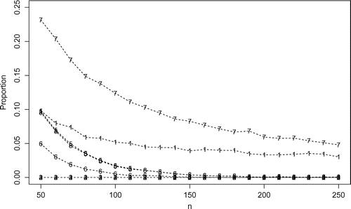
Figure 4. MREs, MSEs related from the estimates of $\mathit{\varphi }=0.5,\mathit{\lambda }=0.7$ and $\mathit{\alpha }=1.5$ for N simulated samples, considering different values of n obtained using the following estimation method 1-MLE, 2-MPS, 3-ADE, 4-RTADE.

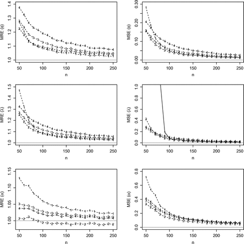
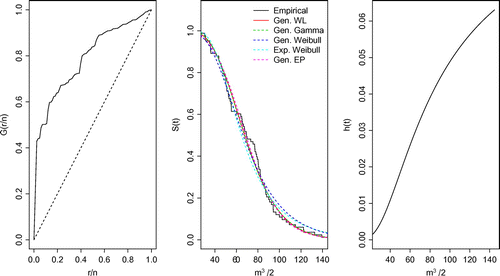
Figure 5. (left panel) the TTT-plot, (middle panel) the fitted survival superimposed to the empirical survival function and (right panels) the hazard function adjusted by GWL distribution.

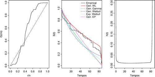
Figure 6. (left panel) the TTT-plot, (middle panel) the fitted survival superimposed to the empirical survival function and (right panels) the hazard function adjusted by GWL distribution.

For this comparison to be meaningful, the estimation procedures need to be performed under same conditions. However, for some particular samples and estimation methods, the numerical techniques do not work well in finding the parameter estimates. Therefore, a rate study is presented to verify the frequency of convergence of the numerical solutions. This procedure is carried out by counting the number of times each estimation fails in finding the numerical solution. In Figure 3 we present the proportion of failure from each method.

From Figure 3, the MLE, LSE, WLSE, ME, and the CME estimators fail in finding the parameter estimates for a significant number of samples. Therefore, such methods are not recommended for estimation of the GLW parameters. Hereafter, we consider the MPS, ADE, RADE estimators due to their better computational stability. The MLE is considered only for illustrative purposes since it is the most used estimation method. Figure 4 presents the MREs, MSEs for the estimates of $\mathit{\varphi },\mathit{\lambda }$ and $\mathit{\alpha }$ using the MLE, MPS, ADE, RADE with N simulated samples and different values of $\mathit{\theta }=(2,0.5,0.1)$ and n. The horizontal lines in both figures correspond to MREs and MSEs being one and zero, respectively.

From these results, the MSE of the MLE, MPS, ADE, and RADE estimators tend to zero for large n and also, as expected, the values of MREs tend to one, i.e. the estimates are consistent and asymptotically unbiased for the parameters. For small sample sizes, the MLE has the largest MSEs. The MPS has smaller MSEs with MREs closer to one for almost all values of n. Additionally, the MPS, ADE, and RADE estimators were the only methods that were able to find $\widehat{\mathit{\varphi }},\widehat{\mathit{\lambda }}$ and $\widehat{\mathit{\alpha }}$ for all the $2\times {10}^6$ generated samples. Therefore, combining all results with the good properties of the MPS method such as consistency, asymptotic efficiency, normality and invariance, we conclude that the MPS estimators are a highly competitive method compared to the maximum likelihood for estimating the parameters of the GWL distribution.

5. Application

In this section, we compare the GWL distribution with other three-parameter lifetime distributions considering two data-sets, the first with bathtub hazard rate and the other with the increasing hazard function. The following lifetime distributions were considered. The GG distribution with p.d.f given by$$\begin{array}{c}\hfill f(t)=\mathit{\alpha }\mathrm{\Gamma }{(\mathit{\varphi })}^{-1}{\mathit{\beta }}^{\mathit{\alpha }\mathit{\varphi }}{t}^{\mathit{\alpha }\mathit{\varphi }-1}{e}^{-{(\mathit{\beta }t)}^{\mathit{\alpha }}}\end{array}$$

where $\mathit{\beta }>0,\mathit{\varphi }>0$ and $\mathit{\alpha }>0$. The GW distribution where the p.d.f is$$\begin{array}{c}\hfill f(t)={(\mathit{\alpha }\mathit{\varphi })}^{-1}{(t/\mathit{\varphi })}^{1/\mathit{\alpha }-1}{(1-\mathit{\lambda }{(t/\mathit{\varphi })}^{1/\mathit{\alpha }})}^{1/\mathit{\lambda }-1}\end{array}$$

where $\mathit{\lambda }\in \mathbb{R},\mathit{\varphi }>0$ and $\mathit{\alpha }>0$. The GEP distribution with p.d.f given by$$\begin{array}{c}\hfill f(t)=\left(\mathit{\alpha }\mathit{\beta }\mathit{\varphi }/{(1-e^{-\mathit{\varphi }})}^{\mathit{\alpha }}\right)e^{-\mathit{\varphi }-\mathit{\beta }t+\mathit{\varphi }exp(-\mathit{\beta }t)}{\left(1-e^{-\mathit{\varphi }+\mathit{\varphi }exp(-\mathit{\beta }t)}\right)}^{\mathit{\alpha }-1}\end{array}$$

where $\mathit{\beta }>0,\mathit{\varphi }>0$ and $\mathit{\alpha }>0$

The EW distribution with p.d.f$$\begin{array}{c}\hfill f(t)=\mathit{\alpha }\mathit{\varphi }{\mathit{\beta }}^{-1}{(t/\mathit{\beta })}^{\mathit{\alpha }-1}exp\left(-{(t/\mathit{\beta })}^{\mathit{\alpha }}\right){\left(1-exp\left(-{(t/\mathit{\beta })}^{\mathit{\alpha }}\right)\right)}^{\mathit{\varphi }-1}\end{array}$$

where $\mathit{\beta }>0,\mathit{\varphi }>0$ and $\mathit{\alpha }>0$.

The TTT-plot (total time on test) is considered in order to verify the behavior of the empirical hazard function (Barlow & Campo, 1975). The TTT-plot is obtained through the plot of [r / n, G(r / n)] where$$\begin{array}{c}\hfill G(r/n)=\left(\sum _{i=1}^r{t}_i+(n-r)t_{(r)}\right)/\sum _{i=1}^n{t}_i,r=1,\dots ,n,i=1,\dots ,n\end{array}$$

and $t_{(i)}$ is the statistical order. If the curve is concave (convex), the hazard function is increasing (decreasing). On the other hand, when it starts convex and then becomes concave (concave and then convex) the hazard function has bathtub (inverse bathtub) shape.

The goodness of fit is checked considering the Kolmogorov–Smirnov (KS) test. This procedure is based on the KS statistic $D_n=sup\left|F_n(t)-F(t;\mathit{\varphi },\mathit{\lambda },\mathit{\alpha })\right|$, where $supt$ is the supremum of the set of distances, $F_n(t)$ is the empirical distribution function and $F(t;\mathit{\alpha },\mathit{\beta },\mathit{\lambda })$ is c.d.f. A hypothesis test is conducted at the $5\%$ level of significance to test whether or not the data come from $F(t;\mathit{\alpha },\mathit{\beta },\mathit{\lambda })$. In this case, the null hypothesis is rejected if the returned p-value is smaller than 0.05.

To carry out the model selection, the following discrimination criterion methods are adopted: AIC (Akaike information criteria) and AICc (Corrected Akaike information criterion) computed, respectively, by $AIC=-2l(\widehat{\mathit{\theta }};\mathit{t})+2k$ and $AICc=AIC+2k(k+1){(n-k-1)}^{-1}$, where k is the number of parameters to be fitted and $\widehat{\mathit{\theta }}$ is estimation of $\mathit{\theta }$. For a set of candidate models for $\mathit{t}$, the best one provides the minimum values.

5.1. Lifetimes data

Aarset (1987) presents the data-set (see Table 1) related to the lifetime in hours of 50 devices on test

Table 1. Lifetimes data (in hours) related to a device on test

0.1	0.2	1	1	1	1	1	2	3	6	7	11	12
18	18	18	18	18	21	32	36	40	45	46	47	50
55	60	63	63	67	67	67	67	72	15	79	82	82
83	84	84	84	85	85	85	85	85	86	86

Figure 5 shows (left panel) the TTT-plot, (middle panel) the fitted survival superimposed to the empirical survival function and (right panels) the hazard function adjusted by GWL distribution. Table 2 presents the AIC and AICc criteria and the p-value from the KS test for all fitted distributions considering the Aarset dataset.

Table 2. Results of AIC and AICc criteria and the p-value from the KS test for all fitted distributions considering the Aarset dataset

Criteria	Gen. WL	Gen. Gamma	Gen. Weibull	Exp. Weibull	Gen. EP
AIC	418.031	448.294	430.055	463.674	486.255
AICc	412.552	442.816	424.576	458.196	480.777
KS	0.5787	0.0115	0.0453	0.0222	0.0302

Table 3. MPS estimates, standard-error and $95\%$ CI for $\mathit{\varphi },\mathit{\lambda }$ and $\mathit{\alpha }$

$\mathit{\theta }$	${\widehat{\mathit{\theta }}}_{MPS}$	S.E($\widehat{\mathit{\theta }}$)	CI${}_{95\%}(\mathit{\theta })$
$\mathit{\varphi }$	0.0057	0.00091	( 0.0039; 0.0075)
$\mathit{\lambda }$	0.0118	0.00003	(0.0117; 0.0118)
$\mathit{\alpha }$	110.4964	6.58144	(97.5971; 123.3958)

Table 4. January average flows (m${}^3$/s) of the Cantareira system

82.0	80.9	102.5	65.3	65.5	47.1	53.0	139.4	82.4	80.2	92.5
50.0	50.4	50.2	36.2	35.9	100.0	94.2	78.1	54.8	86.9	80.1
60.3	26.9	48.5	51.0	51.1	84.5	76.9	69.4	77.3	109.2	55.3
106.3	30.5	94.2	87.3	115.0	70.0	31.3	87.1	35.9	67.7	55.1
89.9	50.1	52.6	82.0	54.1	44.3	69.2	94.4	83.4	122.7	88.1
73.3	35.9	82.4	64.9	90.8	80.4	55.3	31.4	45.7	43.6	45.8
96.8	85.8	43.6	122.3	66.5	41.0	75.4	79.4	34.8	78.8	52.4
77.1	47.0	67.4	132.8	144.9	64.1

Table 5. Results of AIC and AICc criteria and the p-value from the KS test for all fitted distributions considering the data-set related to the january average flows (m${}^3$/s) of the Cantareira system

Criteria	Gen. WL	Gen. Gamma	Gen. Weibull	Exp. Weibull	Gen. EP
AIC	775.431	775.461	777.280	780.304	778.873
AICc	769.735	769.765	771.584	774.608	773.176
KS	0.4683	0.4223	0.3935	0.1654	0.4599

Table 6. ML estimates, standard-error and $95\%$ CI for $\mathit{\varphi },\mathit{\lambda }$ and $\mathit{\alpha }$

$\mathit{\theta }$	${\widehat{\mathit{\theta }}}_{\text{MLE}}$	S.E($\widehat{\mathit{\theta }}$)	CI${}_{95\%}(\mathit{\theta })$
$\mathit{\varphi }$	7.0485	1.5425	(2.3847; 11.7124)
$\mathit{\lambda }$	0.1244	0.0557	(0.1183; 0.1305)
$\mathit{\alpha }$	0.9579	0.1173	(0.9310; 0.9849)

Comparing the empirical survival function with the adjusted distributions, it can be observed that the GWL distribution is as a better fit. This result is also confirmed from the AIC and AICC (see Table 3) since GWL distribution has the minimum values and also the p-values returned from the KS test are greater than 0.05. It should be emphasized that considering a significance level of $5\%$, the others models are not able to fit the proposed data. Table 3 displays the MPS estimates, standard errors, and the confidence intervals (CI) for $\mathit{\varphi },\mathit{\lambda }$ and $\mathit{\alpha }$ of the GWL distribution.

In this section, we consider the ML estimator showing that both MPS or MLE could be used successfully in applications. Figure 6 shows (left panel) the TTT-plot, (middle panel) the fitted survival superimposed to the empirical survival function and (right panels) the hazard function adjusted by GWL distribution. Table 5 presents the AIC and AICc criteria and the p-value from the KS test for all fitted distributions considering the data-set related to the January average flows (m${}^3$/s) of the Cantareira system.

From the empirical survival function and the adjusted distributions, it can be observed that the GWL distribution is better. This result is also confirmed from AIC and AICC since GWL distribution has the minimum values and the p-values returned from the KS test are greater than 0.05. Table 6 displays the ML estimates, standard errors, and the CI for $\mathit{\varphi },\mathit{\lambda }$ and $\mathit{\alpha }$ of the GWL distribution.

5.2. Average flows data

The study of average flows has been proved to be of high importance to protect and maintain aquatic resources in streams and rivers (Reiser, Wesche, & Estes, 1989). In this section, we consider a real data-set related to the average flows (m${}^3$/s) of the Cantareira system during January at São Paulo city in Brazil. It is worth mentioning that the Cantareira system provides water to 9 million people in the São Paulo metropolitan area. The data-set available in Table 4 was obtained from the National Water Agency from 1930 to 2012.

6. Concluding remarks

To summarize, we have proposed a three-parameter lifetime distribution. The GLW distribution is a straightforward generalization of the WL distribution proposed by Ghitany et al. (2011), which accommodates increasing, decreasing, decreasing-increasing-decreasing, bathtub, and unimodal hazard rate making the GWL distribution a flexible model for reliable data. The mathematical properties of this distribution are also discussed.

The estimation procedures for the parameters of GWL distribution are also derived considering eight estimation methods. Since it is not feasible to compare these methods theoretically, we have presented an extensive simulation study in order to identify the most efficient procedure. We observed that the MLE, ME, LSE, WLSE, and the CME estimators fail in finding the parameter estimates for a significant number of samples. The simulations showed that the MPS (maximum product of spacing) is the most efficient method for estimating the parameters of the GWL distribution in comparison to its competitors. Finally, two data-sets were analyzed for illustrative purposes proving that the GWL distribution outperforms several usual three parameter lifetime distributions.

Acknowledgements

We are grateful to the Editorial Board and the reviewers for their valuable comments and suggestions which has improved the manuscript.

Additional information

Funding

The research was partially supported by CNPq, FAPESP, and CAPES of Brazil.

Notes on contributors

P.L. Ramos

P.L. Ramos holds a BSc degree in Statistics and an MSc in Applied and Computational Mathematics from the São Paulo State University, Brazil. He is currently reading for his PhD in Statistics at the Institute for Mathematical Science and Computing, University of São Paulo (USP), Brazil. His main research interests are in survival analysis, Bayesian inference, classical inference, and probability distribution theory.

F. Louzada

F. Louzada is a professor of Statistics at the Institute for Mathematical Science and Computing, University of So Paulo (USP), Brazil. He received his PhD degree in Statistics from the University of Oxford, UK, his MSc degree in Computational Mathematics from USP, Brazil, and his BSc degree in Statistics from UFSCar, Brazil. His main research interests are in survival analysis, data mining, Bayesian inference, classical inference, and probability distribution theory.

Appendix 1

Appendix

The elements of the Fisher information matrix are$$\begin{array}{cc}\hfill I_{\mathit{\varphi },\mathit{\varphi }}& =-E\left[\frac{\mathit{\partial }l(\mathit{\theta };\mathit{t})}{\mathit{\partial }{\mathit{\varphi }}^2}\right]=-\frac{1}{{(\mathit{\lambda }+\mathit{\varphi })}^2}+{\mathit{\psi }}^{\prime }(\mathit{\theta })\hfill \\ \hfill I_{\mathit{\varphi },\mathit{\lambda }}& =-E\left[\frac{\mathit{\partial }l(\mathit{\theta };\mathit{t})}{\mathit{\partial }\mathit{\varphi }\mathit{\partial }\mathit{\lambda }}\right]=-\frac{\mathit{\alpha }}{\mathit{\lambda }}+\frac{1}{{(\mathit{\lambda }+\mathit{\varphi })}^2}\hfill \\ \hfill I_{\mathit{\varphi },\mathit{\alpha }}& =-E\left[\frac{\mathit{\partial }l(\mathit{\theta };\mathit{t})}{\mathit{\partial }\mathit{\varphi }\mathit{\partial }\mathit{\alpha }}\right]=\frac{-\mathit{\alpha }log(\mathit{\lambda })-\mathit{\psi }(\mathit{\varphi })+\mathit{\alpha }log(\mathit{\lambda })-{(\mathit{\lambda }+\mathit{\varphi })}^{-1}}{\mathit{\alpha }}\hfill \\ \hfill I_{\mathit{\lambda },\mathit{\lambda }}& =-E\left[\frac{\mathit{\partial }l(\mathit{\theta };\mathit{t})}{\mathit{\partial }{\mathit{\lambda }}^2}\right]=\frac{\mathit{\alpha }\mathit{\varphi }}{{\mathit{\lambda }}^2}+(\mathit{\alpha }-1){\mathit{\lambda }}^{\mathit{\alpha }-2}(\mathit{\psi }(\mathit{\varphi })-\mathit{\alpha }log(\mathit{\lambda })+{(\mathit{\lambda }+\mathit{\varphi })}^{-1})\hfill \\ \hfill & +E\left[\frac{\mathit{\alpha }{T}^{\mathit{\alpha }}{\mathit{\lambda }}^{\mathit{\alpha }-2}\left((\mathit{\alpha }-2)\mathit{\lambda }-{(\mathit{\lambda }T)}^{\mathit{\alpha }}\right)}{\left(\mathit{\lambda }+{(\mathit{\lambda }T)}^{\mathit{\alpha }}\right)}\right]-\frac{1}{{(\mathit{\lambda }+\mathit{\varphi })}^2}\hfill \\ \hfill I_{\mathit{\alpha },\mathit{\alpha }}& =-E\left[\frac{\mathit{\partial }l(\mathit{\theta };\mathit{t})}{\mathit{\partial }{\mathit{\alpha }}^2}\right]=\frac{\mathit{\varphi }(\mathit{\lambda }+\mathit{\varphi }+1)\left(\mathit{\psi }{(\mathit{\varphi })}^2+\mathit{\psi }(\mathit{\varphi })\right)}{{\mathit{\alpha }}^2(\mathit{\lambda }+\mathit{\varphi })}+\frac{1}{{\mathit{\alpha }}^2}\hfill \\ \hfill & +\frac{2(\mathit{\lambda }+2\mathit{\varphi }+1)\mathit{\psi }(\mathit{\varphi })+2}{{\mathit{\alpha }}^2(\mathit{\lambda }+\mathit{\varphi })}-E\left[\frac{\mathit{\lambda }{(\mathit{\lambda }T)}^{\mathit{\alpha }}log{(\mathit{\lambda }T)}^2}{\left(\mathit{\lambda }+{(\mathit{\lambda }T)}^{\mathit{\alpha }}\right)}\right]\hfill \\ \hfill I_{\mathit{\alpha },\mathit{\lambda }}& =-E\left[\frac{\mathit{\partial }l(\mathit{\theta };\mathit{t})}{\mathit{\partial }\mathit{\alpha }\mathit{\partial }\mathit{\lambda }}\right]=-\frac{\mathit{\varphi }}{\mathit{\lambda }}+\frac{\mathit{\lambda }\left(1+\mathit{\varphi }\mathit{\psi }(\mathit{\varphi })\right)+\mathit{\varphi }\left(1+(\mathit{\varphi }+1)\mathit{\psi }(\mathit{\varphi }+1)\right)}{\mathit{\lambda }(\mathit{\lambda }+\mathit{\varphi })}\hfill \\ \hfill & -E\left[\frac{\left(1+\mathit{\alpha }{\mathit{\lambda }}^{\mathit{\alpha }-1}{T}^{\mathit{\alpha }}\right){(\mathit{\lambda }T)}^{\mathit{\alpha }}log(\mathit{\lambda }T)}{{\left(\mathit{\lambda }+{(\mathit{\lambda }T)}^{\mathit{\alpha }}\right)}^2}\right]+\frac{\left(\mathit{\varphi }+\mathit{\lambda }+1-\frac{1}{\mathit{\alpha }}\right)\mathrm{\Gamma }\left(\mathit{\varphi }+1-\frac{1}{\mathit{\alpha }}\right)}{(\mathit{\lambda }+\mathit{\varphi })\mathrm{\Gamma }(\mathit{\varphi })}\hfill \\ \hfill & -E\left[\frac{\left(\mathit{\alpha }{\mathit{\lambda }}^{\mathit{\alpha }-1}{T}^{\mathit{\alpha }}log(\mathit{\lambda }T)+{(\mathit{\lambda }T)}^{\mathit{\alpha }-1}\right)}{\left(\mathit{\lambda }+{(\mathit{\lambda }T)}^{\mathit{\alpha }}\right)}\right]\hfill \end{array}$$

References

- Aarset, M. V. (1987). How to identify a bathtub hazard rate. IEEE Transactions on Reliability, 36, 106–108.
- Ali, S. (2015). On the bayesian estimation of the weighted lindley distribution. Journal of Statistical Computation and Simulation, 85, 855–880.
- Al-Mutairi, D., Ghitany, M., & Kundu, D. (2015). Inferences on stress-strength reliability from weighted lindley distributions. Communications in Statistics-Theory and Methods, 44, 4096–4113.
- Bakouch, H. S., Al-Zahrani, B. M., Al-Shomrani, A. A., Marchi, V. A., & Louzada, F. (2012). An extended lindley distribution. Journal of the Korean Statistical Society, 41, 75–85.
- Barlow, R. E., & Campo, R. A. (1975). Total time on test processes and applications to failure data analysis (Technical report). Berkeley, CA: DTIC Document.
- Barreto-Souza, W., & Bakouch, H. S. (2013). A new lifetime model with decreasing failure rate. Statistics, 47, 465–476.
- Barreto-Souza, W., & Cribari-Neto, F. (2009). A generalization of the exponential-poisson distribution. Statistics & Probability Letters, 79, 2493–2500.
- Bonferroni, C. (1930). Elementi di statistica generale. Firenze: Seeber.
- Cheng, R. & Amin, N. (1979). Maximum product of spacings estimation with application to the lognormal distribution (Mathematical Report 79-1). Cardiff: University of Wales IST.
- Cheng, R., & Amin, N. (1983). Estimating parameters in continuous univariate distributions with a shifted origin. Journal of the Royal Statistical Society. Series B (Methodological), 45, 394–403.
- Ghitany, M., Al-Mutairi, D., Balakrishnan, N., & Al-Enezi, L. (2013). Power lindley distribution and associated inference. Computational Statistics & Data Analysis, 64, 20–33.
- Ghitany, M., Alqallaf, F., Al-Mutairi, D., & Husain, H. (2011). A two-parameter weighted lindley distribution and its applications to survival data. Mathematics and Computers in Simulation, 81, 1190–1201.
- Ghitany, M., Atieh, B., & Nadarajah, S. (2008). Lindley distribution and its application. Mathematics and Computers in Simulation, 78, 493–506.
- Glaser, R. E. (1980). Bathtub and related failure rate characterizations. Journal of the American Statistical Association, 75, 667–672.
- Luceño, A. (2006). Fitting the generalized pareto distribution to data using maximum goodness-of-fit estimators. Computational Statistics & Data Analysis, 51, 904–917.
- Macdonald, P. (1971). An estimation procedure for mixtures of distribution. Journal of the Royal Statistical Society. Series B (Methodological), 33, 326–329.
- Mazucheli, J., Louzada, F., & Ghitany, M. (2013). Comparison of estimation methods for the parameters of the weighted lindley distribution. Applied Mathematics and Computation, 220, 463–471.
- Mudholkar, G. S., Srivastava, D. K., & Freimer, M. (1995). The exponentiated weibull family: A reanalysis of the bus-motor-failure data. Technometrics, 37, 436–445.
- Mudholkar, G. S., Srivastava, D. K., & Kollia, G. D. (1996). A generalization of the weibull distribution with application to the analysis of survival data. Journal of the American Statistical Association, 91, 1575–1583.
- Popescu, T. D., & Aiordachioaie, D. (2013). Signal segmentation in time-frequency plane using renyi entropy-application in seismic signal processing. In 2013 Conference on Control and Fault-Tolerant Systems (SysTol) (pp. 312–317). Nice: IEEE.
- Ranneby, B. (1984). The maximum spacing method. An estimation method related to the maximum likelihood method. Scandinavian Journal of Statistics, 11, 93–112.
- Reiser, D. W., Wesche, T. A., & Estes, C. (1989). Status of instream flow legislation and practices in north america. Fisheries, 14, 22–29.
- Renyi, A. (1961). On measures of entropy and information. In Fourth Berkeley Symposium on Mathematical Statistics and Probability, 1, 47–561.
- Stacy, E. W. (1962). A generalization of the gamma distribution. The Annals of Mathematical Statistics, 33, 1187–1192.
- Torabi, H., Falahati-Naeini, M., & Montazeri, N. (2014). An extended generalized lindley distribution and its applications to lifetime data. Journal of Statistical Research of Iran, 11, 203–222.
- Wang, M., & Wang, W. (in press). Bias-corrected maximum likelihood estimation of the parameters of the weighted lindley distribution. Communications in Statistics-Simulation and Computation, 46, 530–545.
- Zakerzadeh, H., & Dolati, A. (2009). Generalized lindley distribution. Journal of Mathe-matical Extension, 3, 1–17