A novel approach for numeric study of 2D biological population model

Abstract

In the present paper, the modified cubic B-spline differential quadrature method (MCB-DQM) has been implemented for the numerical computation of two-dimensional biological population model (BPM). The method is based on differential quadrature in which the weighting coefficients are computed by using MCB as a set of basis functions. We present three test problems to confirm the efficiency and accuracy of the method for BPM, which shows that the MCB-DQM solutions are in good agreement with the results obtained by the recent schemes: improved element-free Galerkin method by Zhang et al. and element-free kp-Ritz method by Cheng et al. The order of convergence of MCB-DQM for the solutions of BPM is shown to be quadratic.

Keywords:

• biological population model (BPM)
• differential quadrature method (DQM)
• modified cubic B-splines (MCB)
• SSP-RK54 scheme
• Thomas algorithm

Public Interest Statement

The biological problems received much attention among the researchers due to its key role in the regulation of population of some species. Indeed, the computation of the exact solution each differential equation (DE) is too tough task. Therefore, the development of new schemes for numerical solution of PDEs with accurate, stable and efficient, is of vital importance. Modified cubic B-spline differential quadrature method (MCB-DQM) is implemented for solving two-dimensional biological population model (BPM). This is a new DQM with modified cubic B-splines as new set of basis functions. Three problems are considered to confirm the efficiency and accuracy of the method for BPM. MCB-DQM solutions are in good agreement with the recent results obtained using improved element-free Galerkin method by Zhang et al. and element-free kp-Ritz method by Cheng et al. The order of convergence of the proposed scheme is quadratic.

1. Introduction

The dispersal or emigration plays a significant role in the regulation of population of some species. In the recent years, the biological problems have been received a much attention among the researchers due to its key role in the regulation of population of some species. The diffusion of a biological species in a region ${\mathbb{R}}^2$ is described by three functions: (i) population density $\mathit{\rho }(\mathbf{x},t)$, (ii) diffusion velocity $\mathit{\nu }(\mathbf{x},t)$ and (iii) population supply $\mathit{\sigma }(\mathbf{x},t)$ (Gurtin & Maccamy, 1977), where $\mathbf{x}=(x,y)\in {\mathbb{R}}^2$ and t is time.

The population density $\mathit{\rho }$ represents the number of individuals per unit volume at $(\mathbf{x},t)$, and it’s integral over any sub-region $\mathbb{D}$ of region ${\mathbb{R}}^2$ gives the total population of $\mathbb{D}$ at time t whereas $\mathit{\sigma }(\mathbf{x},t)$ denotes the rate at which individuals are supplied in per unit volume at position $\mathbf{x}$ at time t by births and deaths. The diffusion velocity $\mathit{\nu }(\mathbf{x},t)$ represents the average velocity of the individuals occupying the position $\mathbf{x}$ at the time t, and it represents the flow of population from one point to another point. The entities $\mathit{\rho },\mathit{\nu }$ and $\mathit{\sigma }$ must be consistent with law of population balance (Gurney & Nisbet, 1975; Lu, 2000), given below in Equation (1): for every regular sub-region $\mathbb{D}$ of ${\mathbb{R}}^2$ at time t (1) $$\begin{array}{c}\hfill \frac{\text{d}}{\text{d}t}\underset{\mathbb{D}}{\int }\mathit{\rho }\text{d}V+\underset{\mathit{\partial }\mathbb{D}}{\int }\mathit{\rho }\mathit{\nu }·\mathbf{n}\text{d}V=\underset{\mathbb{D}}{\int }\mathit{\sigma }\text{d}V\end{array}$$(1)

where $\mathbf{n}$ is the outward unit normal to the boundary $\mathit{\partial }\mathbb{D}$ of the region $\mathbb{D}$. The law (1) shows that “the sum of the rate of change of population of $\mathbb{D}$ and the rate at which the individuals leave the region $\mathbb{D}$ across its boundary $\mathit{\partial }\mathbb{D}$ is equal to the rate at which the individuals are supplied directly to the region $\mathbb{D}$”.

Table 1. Comparison of numerical solution of Example 1 at $x=0.5,y=0.5$

	$t=0.1$	$t=0.2$	$t=0.3$	$t=0.4$	$t=0.5$
MCB-DQM	1.26282	1.14254	1.03381	0.93543	0.84641
IEFGM (Zhang et al., 2014)	1.2574	1.1382	1.0302	0.9325	0.8440
Exact	1.2628	1.1426	1.0339	0.9355	0.8465
CPU(s)	0.31	0.59	0.90	1.22	1.51

Table 2. The errors in Example 1 at different time levels $t\le 0.5$

$M=N$	Errors	$t=0.1$	$t=0.2$	$t=0.3$	$t=0.4$	$t=0.5$
13	$L_2$	2.689E-05	2.391E-05	2.141E-05	1.929E-05	1.747E-05
	$L_{\infty }$	1.052E-04	8.604E-05	7.037E-05	5.756E-05	4.709E-05
	CPU(s)	0.33	0.64	0.96	1.29	1.58
26	$L_2$	1.479E-05	1.183E-05	9.458E-06	7.568E-06	6.069E-06
	$L_{\infty }$	1.069E-04	8.716E-05	7.113E-05	5.806E-05	4.740E-05
	CPU(s)	2.31	4.62	6.81	9.14	11.14

Table 3. The errors in Example 1 for large time levels $5\le t\le 20$ with $h_x=h_y=1/12$

Errors	$t=5$	$t=10$	$t=15$	$t=20$
$L_2$	2.33E-07	1.57E-09	1.06E-11	7.14E-14
$L_{\infty }$	3.40E-07	2.30E-09	1.55E-11	1.04E-13
CPU(s)	15.17	30.31	45.34	61.43

Table 4. Rate of convergence (ROC) of Example 1

	$t=0.4$			$t=0.1$
$M=N$	$L_2$	ROC	CPU(s)	$L_2$	ROC	CPU(s)
5	1.17E-04		0.16	1.56E-04		0.04
10	2.85E-05	2.03	0.79	3.85E-05	2.02	0.20
15	1.22E-05	2.09	2.19	1.88E-05	1.76	0.60
20	8.23E-06	1.38	4.80	1.40E-05	1.02	1.29

Table 5. Errors in BPM given in Example 2 at $0\le t\le 1.0$ for different time steps and $h_x=h_y=0.1$

t	$▵t=0.001$			$▵t=0.0005$			$▵t=0.0001$
	$L_2$	$L_{\infty }$	CPU(s)	$L_2$	$L_{\infty }$	CPU(s)	$L_2$	$L_{\infty }$	CPU(s)
0.1	1.172E-04	3.689E-04	0.03	5.872E-05	1.827E-04	0.06	4.156E-05	6.096E-05	0.19
0.5	1.179E-04	3.691E-04	0.09	5.897E-05	1.828E-04	0.20	4.380E-05	6.265E-05	0.94
1.0	1.184E-04	3.694E-04	0.20	5.901E-05	1.829E-04	0.40	4.334E-05	6.164E-05	1.92

For $\mathit{\sigma }=\mathit{\sigma }(\mathit{\rho })$ and $\mathit{\nu }=-\mathit{\lambda }(\mathit{\rho })\mathrm{\nabla }\mathit{\rho }$, where $\mathit{\lambda }(\mathit{\rho })>0$ for $\mathit{\rho }>0$ and $\mathrm{\nabla }$ is the Laplace operator, the following nonlinear degenerate parabolic partial differential equation (DE) for $\mathit{\rho }$ is reduced to(2) $$\begin{array}{c}\hfill \frac{\mathit{\partial }\mathit{\rho }}{\mathit{\partial }t}={\mathrm{\nabla }}^2(\mathit{\varphi }(\mathit{\rho }))+\mathit{\sigma }(\mathit{\rho }),\end{array}$$(2)

where ${\mathrm{\nabla }}^2\equiv \frac{{\mathit{\partial }}^2}{\mathit{\partial }{x}^2}+\frac{{\mathit{\partial }}^2}{\mathit{\partial }{y}^2}$ and $\mathit{\varphi }(\mathit{\rho })$ be function of $\mathit{\rho }$ (Gurtin & Maccamy, 1977). In Gurney and Nisbet (1975), $\mathit{\sigma }(\mathit{\rho })$ is used as a special case in the modeling of the population of animals. The movements were made generally either by mature animals driven by mature invaders or by the young animals just reaching maturity moving out of their parental territory to establish breeding territory of their own. In each case, it is much more probable to consider that they will be directed toward nearby vacant territory. Therefore, in this model, the movement will take place almost exclusively down the population density gradient and will be more rapid at high population densities than at low ones. To model this situation, the authors further assumed a walk through a rectangular grid, in which at each step, an animal may either stay at its present location or may move toward the lowest population density (Gurney & Nisbet, 1975). The probability distribution between these two possibilities being determined by the magnitude of the population density gradient at the grid side is concerned. This model is correspond to Equation (2) with $\mathit{\varphi }(\mathit{\rho })={\mathit{\rho }}^2$ as(3) $$\begin{array}{c}\hfill \frac{\mathit{\partial }\mathit{\rho }}{\mathit{\partial }t}={\mathrm{\nabla }}^2({\mathit{\rho }}^2)+\mathit{\sigma }(\mathit{\rho }).\end{array}$$(3)

Some properties of Equation (3) such as Holder-estimates and its solutions were studied in Lu (2000). Equation (3) is the generalization of the following lows:

(a)	For $\mathit{\sigma }(\mathit{\rho })=c\mathit{\rho }$, c is a constant (Malthusian Law Gurtin and Maccamy, 1977).
(b)	For $\mathit{\sigma }(\mathit{\rho })=c_1\mathit{\rho }-c_2{\mathit{\rho }}^2$, where $c_1,c_2>0$ are constant (Verhulst Law Gurtin & Maccamy, 1977).
(c)	For $\mathit{\sigma }(\mathit{\rho })=c{\mathit{\rho }}^{\mathit{\alpha }}$ with $c\ge 0$ and $0<\mathit{\alpha }<1$ (Porous media Bear, 1972; Okubo, 1980).

Consider two-dimensional (2D) biological population model (BPM) (3) with $\mathit{\sigma }(\mathit{\rho })=h{\mathit{\rho }}^{\mathit{\alpha }}(1-r{\mathit{\rho }}^{\mathit{\beta }})$ (Zhang, Deng, & Liew, 2014) as follows:(4) $$\begin{array}{c}\hfill \left\{\begin{array}{ccc}\frac{\mathit{\partial }\mathit{\rho }}{\mathit{\partial }t}\hfill & ={\mathrm{\nabla }}^2({\mathit{\rho }}^2)+h{\mathit{\rho }}^{\mathit{\alpha }}(1-r{\mathit{\rho }}^{\mathit{\beta }}),\hfill & \forall (\mathbf{x},t)\in \mathit{\partial }\mathbb{D}\times (0,T],\hfill \\ \mathit{\rho }(\mathbf{x},0)\hfill & ={\mathit{\rho }}^0(\mathbf{x}),\hfill & \forall \mathbf{x}\in \mathbb{D},\hfill \end{array}\right.\end{array}$$(4)

where $\mathbb{D}=[a,b]\times [c,d]$, and $h,\mathit{\alpha },\mathit{\beta }$ and r are real numbers. The boundary conditions are taken as(5) $$\begin{array}{c}\hfill \left\{\mathit{\rho }(\mathbf{x},t)=\mathit{\psi }(\mathbf{x},t),\forall (\mathbf{x},t)\in \mathit{\partial }\mathbb{D}\times (0,T].\right.\end{array}$$(5)

In the recent years, a lot of numerical techniques have been developed for the numerical computation of time-dependent partial DEs (Arora, Mittal, & Singh, 2014; Arora & Singh, 2013; Cheng, Zhang, & Liew, 2014; Shivanian, 2013; Singh & Kumar, 2016c; Srivastava & Singh, 2014; Zhang et al., 2014). The existence, regularity and uniqueness of the weak solutions for degenerate parabolic equations (see, Aronson, 1986; Dibnedetto, 1993; Giuggioli & Kenkre, 2003; Gurney & Nisbet, 1975; Gurtin & Maccamy, 1977; Jager & Lu, 1997; Lu, 2000). The analytical solutions for time-fractional order population problems were obtained using fractional reduced transform method (Singh & Kumar, 2016a,2016b; Singh & Srivastava, 2015; Srivastava, Mishra, Kumar, Singh, & Awasthi, 2014) by Srivastava, Kumar, Awasthi, and Singh (2014). The computation of various type of population problems is done by using homotopy perturbation method (HPM) (Liu, Li, & Zhang, 2011; Roul, 2010), homotopy analysis method (HAM) (Arafa, Rida, & Mohamed, 2011), and variational iteration method (Shakeri & Dehghan, 2006). A meshless local radial point interpolation numerical method to simulate a nonlinear partial integro-DE arising in population dynamics is given by Shivanian (2013). Recently, the numerical computation of BPM model (4) is done by Cheng et al. (2014) using element-free kp-Ritz method, and by Zhang et al. (2014) using improved element-free Galerkin method (IEFGM).

Table 6. Errors in BPM given in Example 2 at $0\le t\le 1.0$ with $▵t=0.0001$

$h_x=h_y$	Errors	$t=0.1$	$t=0.2$	$t=0.5$	$t=1.0$
0.03	$L_2$	6.43E-06	6.39E-06	6.36E-06	6.31E-06
	$L_{\infty }$	3.70E-05	3.69E-05	3.69E-05	3.69E-05
	CPU(s)	4.84	9.76	24.4	49.11
0.04	$L_2$	9.46E-06	9.53E-06	9.56E-06	9.39E-06
	$L_{\infty }$	3.65E-05	3.65E-05	3.65E-05	3.65E-05
	CPU(s)	2.23	4.48	11.24	22.52

Table 7. The errors in Example 2 for large time levels $5\le t\le 20$ with $h_x=h_y=1/12$

Errors	$t=5$	$t=10$	$t=15$	$t=20$
$L_2$	2.71E-05	2.50E-05	2.33E-05	2.19E-05
$L_{\infty }$	3.64E-05	3.65E-05	3.65E-05	3.66E-05
CPU(s)	12.14	30.22	45.67	60.94

Table 8. Rate of convergence of Example 2

	$t=1.0$			$t=0.5$
$M=N$	$L_2$	ROC	CPU(s)	$L_2$	ROC	CPU(s)
6	1.66E-04		0.36	1.67E-04		0.20
11	4.33E-05	2.21	1.90	4.38E-05	2.21	0.94
16	1.78E-05	2.38	5.45	1.80E-05	2.37	2.70
21	9.46E-06	2.32	12.00	9.53E-06	2.34	5.93
26	6.84E-06	1.52	22.33	6.34E-06	1.91	11.4

Table 9. Comparison of numerical solution of Example 3 at $x=0.5,y=0.5$

	$t=0.1$	$t=0.2$	$t=0.3$	$t=0.4$	$t=0.5$
MCB-DQM	0.5078	0.5170	0.5273	0.5379	0.5488
IEFGM (Zhang et al., 2014)	0.5069	0.5165	0.5268	0.5373	0.5481
Exact	0.5101	0.5204	0.5309	0.5416	0.5526
CPU(s)	0.31	0.61	0.94	1.20	1.48

Table 10. The errors in Example 3 for large time levels $2\le t\le 10$ with $h_x=h_y=1/12$

Errors	$t=2$	$t=5$	$t=8$	$t=10$
$L_2$	7.94E-03	1.50E-02	3.06E-02	2.07E-02
$L_{\infty }$	2.31E-03	4.10E-03	1.13E-02	9.34E-02
CPU(s)	5.87	14.84	23.79	29.60

The main aim of this paper is to implement “modified cubic B-spline differential quadrature method (MCB-DQM)” (Arora & Singh, 2013; Singh & Arora, 2014; Singh & Bianca, 2016) for the numerical computation of 2D BPM. The scheme is based on differential quadrature where the modified cubic-B-spline functions are used as set of basis functions to determine the weighting coefficients. The MCB-DQM is used to convert the given system of PDEs into a system of first order ODEs, in time. The resulting system of ODEs is solved using the SSP-RK54 scheme. Three test problems are considered to demonstrate the accuracy and utility of the method. The maximum absolute errors $L_{\infty }$ and $L_2$ errors in the MCB-DQM solutions have been compared with the errors due to some recent exiting schemes.

The article is organized as follows. In Section 2, the description of the MCB-DQM is given. In Sections 3, procedure for implementation of method is described. Three numerical examples are given to establish the applicability and accuracy of the proposed method in Section . Section 5 concludes our study.

2. Description of MCB-DQM

Bellman, Kashef, and Casti (1972) have introduced the DQM. DQM is an approximation to the derivatives of a function that is obtained by means of the weighted sum of the functional values at certain discrete points. In DQM, the weighting coefficients are evaluated using various test functions such as spline functions, sinc function, Lagrange interpolation polynomials, modified (extended) cubic B-spline, etc. (Arora & Singh, 2013; Korkmaz & Dag, 2011,2013; Quan & Chang, 1989a,1989b; Shu, Chen, Xue, & Du, 2001; Shu & Richards, 1992; Singh, Arora, & Singh, 2016; Singh & Arora, 2014; Singh & Kumar, 2016c; Zhong, 2004). The weighting coefficients are dependent on the spatial grid spacing only, so one can assume NM grid points on the rectangle $\mathbb{D}=[a,b]\times [c,d]$ distributed uniformly, that is, $a=x_1<x_2,\dots ,x_{N-1}<x_N=b$ with $h_x=x_{i+1}-x_i$, and $c=y_1<y_2,\dots ,y_{M-1}<y_M=d$ with $h_y=y_{i+1}-y_i$. The solution $\mathit{\rho }(x,y,t)$ at any time on the knot $(x_i,y_j)$ is $\mathit{\rho }(x_i,y_j,t)$ for $i=1,\dots ,N$ and $j=1,\dots ,M.$

The approximate value of nth-order partial derivative of the function $\mathit{\rho }(x,y,t)$ with respect to x at $(x_i,y_j)$ is given by(6) $$\begin{array}{c}\hfill \frac{{\mathit{\partial }}^n{\mathit{\rho }}_{ij}}{\mathit{\partial }{x}^n}=\sum _{k=1}^N{a}_{ik}^{(n)}{\mathit{\rho }}_{kj},i=1,2,\dots ,N,\end{array}$$(6)

and the approximate value of mth-order partial derivative of the function $\mathit{\rho }(x,y,t)$ with respect to y at $(x_i,y_j)$ is given by(7) $$\begin{array}{c}\hfill \frac{{\mathit{\partial }}^m{\mathit{\rho }}_{ij}}{\mathit{\partial }{y}^m}=\sum _{k=1}^M{b}_{jk}^{(m)}{\mathit{\rho }}_{ik},j=1,2,\dots ,M,\end{array}$$(7)

where ${\mathit{\rho }}_{ij}=\mathit{\rho }(x_i,y_j,t)$, and $a_{ij}^{(n)}$ and $b_{ij}^{(m)}$ denote the weighting coefficients of the partial derivatives $\frac{{\mathit{\partial }}^n{\mathit{\rho }}_{ij}}{\mathit{\partial }{x}^n}$ and $\frac{{\mathit{\partial }}^m{\mathit{\rho }}_{ij}}{\mathit{\partial }{y}^m}$ at $(x_i,y_j)$ respectively.

The cubic B-spline basis functions at the knots are defined as follows(8) $$\begin{array}{c}\hfill {\mathit{\phi }}_j(x)=\frac{1}{h_x^3}\left\{\begin{array}{cc}{(x-x_{j-2})}^3\hfill & x\in [x_{j-2},x_{j-1})\hfill \\ {(x-x_{j-2})}^3-4{(x-x_{j-1})}^3\hfill & x\in [x_{j-1},x_j)\hfill \\ {(x_{j+2}-x)}^3-4{(x_{j+1}-x)}^3\hfill & x\in [x_j,x_{j+1})\hfill \\ {(x_{j+2}-x)}^3\hfill & x\in [x_{j+1},x_{j+2})\hfill \\ 0\hfill & \text{otherwise},\hfill \end{array}\right.\end{array}$$(8)

where $\{{\mathit{\phi }}_0,{\mathit{\phi }}_1,\dots ,{\mathit{\phi }}_N,{\mathit{\phi }}_{N+1}\}$ forms a basis over the interval [a, b].

Lemma 1

The numerical values of ${\mathit{\phi }}_i$ and its derivatives ${\mathit{\phi }}_i^{\prime },{\mathit{\phi }}_i^{″}$ at j-th nodal point are evaluated as$$\begin{array}{c}\hfill {\mathit{\phi }}_i(x_j)=\left\{\begin{array}{cc}4,\hfill & \text{if}i-j=0\hfill \\ 1,\hfill & \text{if}i-j=\pm 1\hfill \\ 0,\hfill & \text{else}\hfill \end{array}\right.;{\mathit{\phi }}_i^{\prime }(x_j)=\left\{\begin{array}{cc}\pm 3/h_x,\hfill & i-j=\pm 1\hfill \\ 0,\hfill & \text{else}\hfill \end{array}\right.;{\mathit{\phi }}_i^{″}(x_j)=\left\{\begin{array}{cc}-12/h_x^2,\hfill & i-j=0\hfill \\ 6/h_x^2,\hfill & i-j=\pm 1\hfill \\ 0\hfill & \text{else}.\hfill \end{array}\right..\end{array}$$

The modified cubic B-spline basis functions at the knots are defined from Equation (8) in such a way that the resulting matrix system of equations remain diagonally dominant (Arora & Singh, 2013):(9) $$\begin{array}{c}\hfill \left.\begin{array}{cc}{\mathit{\varphi }}_1(x)\hfill & ={\mathit{\phi }}_1(x)+2{\mathit{\phi }}_0(x)\hfill \\ {\mathit{\varphi }}_2(x)\hfill & ={\mathit{\phi }}_2(x)-{\mathit{\phi }}_0(x)\hfill \\ {\mathit{\varphi }}_j(x)\hfill & ={\mathit{\phi }}_j(x)\text{for}j=3,\dots ,N-2\hfill \\ {\mathit{\varphi }}_{N-1}(x)\hfill & ={\mathit{\phi }}_{N-1}(x)-{\mathit{\phi }}_{N+1}(x)\hfill \\ {\mathit{\varphi }}_N(x)\hfill & ={\mathit{\phi }}_N(x)+2{\mathit{\phi }}_{N+1}(x)\hfill \end{array}\right\}\end{array}$$(9)

where $\{{\mathit{\varphi }}_1,{\mathit{\varphi }}_2,\dots ,{\mathit{\varphi }}_N\}$ forms a basis over the interval [a, b].

2.1. Computation of the weighting coefficients $a_{ij}^{(r)}$ and $b_{ij}^{(r)}(r=1,2)$

To find the weighting coefficients $a_{ij}^{(1)}$, the modified cubic B-spline ${\mathit{\varphi }}_k(x)$, $k=1,2,\dots ,N$ is used in Equation (6) due to fixed y axis. The first-order derivative approximation at the grid point $(x_i,y_j)$ is(10) $$\begin{array}{c}\hfill {\mathit{\varphi }}_k^{\prime }(x_i)=\sum _{j=1}^N{a}_{ij}^{(1)}{\mathit{\varphi }}_k(x_j),k=1,\dots ,N.\end{array}$$(10)

By Lemma 1 and Equations (9) and (10) is reduced into a tridiagonal system of linear equations(11) $$\begin{array}{c}\hfill \mathrm{\Phi }\overrightarrow{a}[i]=\overrightarrow{H}[i],\text{for}i=1,\dots ,N,\end{array}$$(11)

where $\mathrm{\Phi }=[{\mathit{\varphi }}_{ij}]$ is the coefficient matrix of order N whose ith row is given by $\mathrm{\Phi }[i]=[{\mathit{\varphi }}_{i1},{\mathit{\varphi }}_{i2},{\mathit{\varphi }}_{i3},\dots ,{\mathit{\varphi }}_{iN}]$, $\overrightarrow{a}[i]$ denotes the weighting coefficient vector corresponding to grid point $x_i$, that is, $\overrightarrow{a}[i]={\left[a_{i1}^{(1)},a_{i2}^{(1)},\dots ,a_{iN}^{(1)}\right]}^T$, and the coefficient vector $\overrightarrow{H}[i]={\left[h_{i1},h_{i2},\dots ,h_{iN}\right]}^T$ corresponding to $x_i$, $i=1,2,\dots ,N$ are evaluated as$$\begin{array}{c}\hfill \overrightarrow{H}[1]=\left[\begin{array}{c}-6/h_x\\ 6/h_x\\ 0\\ ⋮\\ \\ 0\\ 0\end{array}\right],\overrightarrow{H}[2]=\left[\begin{array}{c}-3/h_x\\ 0\\ 3/h_x\\ 0\\ ⋮\\ \\ 0\end{array}\right],\dots ,\overrightarrow{H}[N-1]=\left[\begin{array}{c}0\\ ⋮\\ \\ 0\\ -3/h_x\\ 0\\ 3/h_x\end{array}\right],\text{and}\overrightarrow{H}[N]=\left[\begin{array}{c}0\\ \\ ⋮\\ \\ 0\\ -6/h_x\\ 6/h_x\end{array}\right].\end{array}$$

Now, we apply the well-known “Thomas algorithm” to solve the resulting tridiagonal system of equations which provides the vector $\overrightarrow{a}[i]$, that is, the weighting coefficients $a_{i1}^{(1)},a_{i2}^{(1)},\dots ,a_{iN}^{(1)}$, for $i=1,\dots N$.

Figure 1. The absolute errors BPM in Example 1 at different time levels $t\le 1$ with parameters $h_x=h_y=0.04,▵t=0.0001$.

Figure 2. The approximate solution of BPM in Example 1 at different time levels $t\le 1$ with parameters $h_x=h_y=0.04,▵t=0.0001$.

Figure 3. Contour and surface plot of absolute errors of $\mathit{\rho }(\mathbf{x},t)$ given in Example 2 for $t=0.1,0.5,1$ with parameters $h_x=h_y=0.05,▵t=0.0001$.

Figure 4. The behavior of $\mathit{\rho }(\mathbf{x},t)$ in Example 2 for $t=0.1,0.5,1$ with parameters $h_x=h_y=0.05,▵t=0.0001$.

Figure 5. Contour plot of absolute errors of $\mathit{\rho }(\mathbf{x},t)$ in Example 3 for $t=0.1,0.2,0.3,0.5$ with parameters $h_x=h_y=0.05,▵t=0.0001$.

Figure 6. Surface behavior of BPM as given in Example 3 for $t=0:1;0:2;0:3;0:5$ with parameters $h_x=h_y=0:05;▵t=0:0001$.

Similarly, the weighting coefficients $b_{ij}^{(1)}$ can be computed by means of the modified cubic B-spline ${\mathit{\varphi }}_k(y)$, $k=1,2,\dots ,M$ in Equation (7).

Using the coefficients $a_{ij}^{(1)}$ and $b_{ij}^{(1)}$, the weighting coefficients of higher order spatial derivatives can be obtained using the Shu’s (2000) recursive formulae(12) $$\begin{array}{c}\hfill \left.\begin{array}{ccccc}{a}_{ij}^{(r)}\hfill & =r\left[a_{ij}^{(1)}{a}_{ii}^{(r-1)}-\frac{a_{ij}^{(r-1)}}{x_i-x_j}\right]\hfill & \text{if}i\ne j,\text{and}{a}_{ii}^{(r)}\hfill & =-\sum _{i=1,i\ne j}^N{a}_{ij}^{(r-1)},\hfill & \text{for}i,j=1,2,\dots ,N.\hfill \\ b_{ij}^{(r)}\hfill & =r\left[b_{ij}^{(1)}{b}_{ii}^{(r-1)}-\frac{b_{ij}^{(r-1)}}{y_i-y_j}\right]\hfill & \text{if}i\ne j,\text{and}{b}_{ii}^{(r)}\hfill & =-\sum _{i=1,i\ne j}^N{b}_{ij}^{(r-1)},\hfill & \text{for}i,j=1,2,\dots ,M.\hfill \end{array}\right\}\end{array}$$(12)

where r represents the order of the spatial derivative, $a_{ij}^{(r)}$ and $b_{ij}^{(r)}$ are the weighting coefficients of rth-order partial derivatives of u(x, y, t) at the point $(x_i,y_j)$ with respect to x and y, respectively. In particular, the weighting coefficients $a_{ij}^{(2)},b_{ij}^{(2)}$ of order 2 can be obtained by taking $r=2$ in (12).

3. Implementation of MCB-DQM for 2D BPM

After putting the values of the spatial derivatives approximated using MCB-DQM, Equation (4) can be rewritten as(13) $$\begin{array}{c}\hfill \left\{\begin{array}{cc}\frac{\text{d}{\mathit{\rho }}_{ij}}{\text{d}t}\hfill & =2\left({\mathit{\rho }}_{ij}\sum _{k=1}^N{a}_{ik}^{(2)}{\mathit{\rho }}_{kj}+{\left(\sum _{k=1}^N{a}_{ik}^{(1)}{\mathit{\rho }}_{kj}\right)}^2+{\mathit{\rho }}_{ij}\sum _{k=1}^M{b}_{jk}^{(2)}{\mathit{\rho }}_{ik}+{\left(\sum _{k=1}^M{b}_{jk}^{(1)}{\mathit{\rho }}_{ik}\right)}^2\right)+\mathit{\sigma }({\mathit{\rho }}_{ij})\hfill \\ {\mathit{\rho }}_{ij}(t=0)\hfill & ={\mathit{\rho }}_{ij}^0,1\le i\le N,1\le j\le M,\hfill \end{array}\right.\end{array}$$(13)

where ${\mathit{\rho }}_{ij}=\mathit{\rho }(x_i,y_j,t)$ and $\mathit{\sigma }({\mathit{\rho }}_{ij})=h{\mathit{\rho }}_{ij}^{\mathit{\alpha }}(1-r{\mathit{\rho }}_{ij}^{\mathit{\beta }})$. On implementing the conditions (5), Equation (13) reduced to(14) $$\begin{array}{c}\hfill \left\{\begin{array}{ccc}\frac{\text{d}{\mathit{\rho }}_{ij}}{\text{d}t}\hfill & =L({\mathit{\rho }}_{ij})\hfill & \\ {\mathit{\rho }}_{ij}(t=0)\hfill & ={\mathit{\rho }}_{ij}^0,\hfill & 2\le i\le N-1,2\le j\le M-1,\hfill \end{array}\right.\end{array}$$(14)

where L is nonlinear differential operator defined by$$\begin{array}{cc}\hfill L({\mathit{\rho }}_{ij})& =2\left({\mathit{\rho }}_{ij}\left(\sum _{k=2}^{N-1}{a}_{ik}^{(2)}{\mathit{\rho }}_{kj}+\sum _{k=2}^{M-1}{b}_{jk}^{(2)}{\mathit{\rho }}_{ik}\right)+{\left({\mathit{\epsilon }}_{ij}+\sum _{k=2}^{N-1}{a}_{ik}^{(1)}{\mathit{\rho }}_{kj}\right)}^2+{\left({\mathit{\delta }}_{ij}+\sum _{k=2}^{M-1}{b}_{jk}^{(1)}{\mathit{\rho }}_{ik}\right)}^2\right)+S_{ij},\hfill \\ \hfill {\mathit{\epsilon }}_{ij}& =a_{i1}^{(1)}{\mathit{\rho }}_{1j}+a_{iN}^{(1)}{\mathit{\rho }}_{Nj};{\mathit{\delta }}_{ij}=b_{j1}^{(1)}{\mathit{\rho }}_{i1}+b_{jM}^{(1)}{\mathit{\rho }}_{iM};\hfill \\ \hfill S_{ij}& =2{\mathit{\rho }}_{ij}\left(a_{i1}^{(2)}{\mathit{\rho }}_{1j}+a_{iN}^{(2)}{\mathit{\rho }}_{Nj}+b_{j1}^{(2)}{\mathit{\rho }}_{i1}+b_{jM}^{(2)}{\mathit{\rho }}_{iM}\right)+h{\mathit{\rho }}_{ij}^{\mathit{\alpha }}(1-r{\mathit{\rho }}_{ij}^{\mathit{\beta }}).\hfill \end{array}$$

The resulting system of initial values problem (14) can be solved by various schemes available, in literature. Strong stability preserving time discretization methods were introduced to address the need for nonlinear stability properties in the time discretization, as well as the spatial discretization, of hyperbolic Partial DEs. Strong stability preserving Runge-Kutta (SSP-RK) schemes have some excellent properties such as large regions of absolute stability and low storage, SSP-RK54 is strongly stable scheme with Euler time discretizations for nonlinear hyperbolic PDEs (see Gottlieb, 2005; Spiteri & Ruuth, 2002,2004 and the papers therein). This is why, we prefer SSP-RK54 scheme as defined below, to solve the system of first-order ODEs (14):$$\begin{array}{cc}\hfill {\mathit{\rho }}^{(1)}& ={\mathit{\rho }}^m+0.391752226571890▵tL({\mathit{\rho }}^m)\hfill \\ \hfill {\mathit{\rho }}^{(2)}& =0.444370493651235{\mathit{\rho }}^m+0.555629506348765{\mathit{\rho }}^{(1)}+0.368410593050371▵tL({\mathit{\rho }}^{(1)})\hfill \\ \hfill {\mathit{\rho }}^{(3)}& =0.620101851488403{\mathit{\rho }}^m+0.379898148511597{\mathit{\rho }}^{(2)}+0.251891774271694▵tL({\mathit{\rho }}^{(2)})\hfill \\ \hfill {\mathit{\rho }}^{(4)}& =0.178079954393132{\mathit{\rho }}^m+0.821920045606868{\mathit{\rho }}^{(3)}+0.544974750228521▵tL({\mathit{\rho }}^{(3)})\hfill \\ \hfill {\mathit{\rho }}^{m+1}& =0.517231671970585{\mathit{\rho }}^{(2)}+0.096059710526147{\mathit{\rho }}^{(3)}+0.063692468666290▵tL({\mathit{\rho }}^{(3)})\hfill \\ \hfill & +0.386708617503269{\mathit{\rho }}^{(4)}+0.226007483236906▵tL({\mathit{\rho }}^{(4)})\hfill \end{array}$$

Lemma 2

(Prenter, 1989)   If the function $u\in C^4[a,b]$ such that(15) $$\begin{array}{c}\hfill u(x)=\sum _{j=1}^{N_x}{\mathit{\varphi }}_j(x)u(x_j)+E(x),\end{array}$$(15)

where ${\mathit{\varphi }}_j(x)$ is the cubic B-spline function. Then for any partition of [a, b] with the grids distributed uniformly

(i)	${\left|E(x)\right|}_{\infty }\le \frac{5}{384}{h}_x^4{\left|u^4(x)\right|}_{\infty }$;
(ii)	$|E^{(1)}{(x)|}_{\infty }\le \frac{\sqrt{3}+9}{216}{h}_x^3{\left|u^4(x)\right|}_{\infty }$;
(iii)	$|E^{(2)}{(x)|}_{\infty }\le \frac{5}{12}{h}_x^2{\left|u^4(x)\right|}_{\infty }$.

On setting $a_{ij}^{(1)}={\left.\frac{\text{d}{\mathit{\varphi }}_j(x)}{\text{d}x}\right|}_{x=x_i}$ and $a_{ij}^{(2)}={\left.\frac{{\text{d}}^2{\mathit{\varphi }}_j(x)}{\text{d}{x}^2}\right|}_{x=x_i}$, and if $\mathit{\rho }\in C^4(\mathbb{D},\mathbb{D})$, then from Lemma 2, we get

(a)	$$\begin{array}{c}\hfill \left|\frac{\mathit{\partial }{\mathit{\rho }}_{ij}}{\mathit{\partial }x}-\sum _{k=1}^N{a}_{ik}^{(n)}{\mathit{\rho }}_{kj}\right|\le \frac{\sqrt{3}+9}{216}{h}^3{M}_4\equiv O(h^3),\end{array}$$ where $h=max\{h_x,h_y\}$ and $M_4=max\left\{|{\mathit{\rho }}_{ij}^{(4)}|:1\le i\le N,1\le j\le M\right\}.$
(b)	$\left|\frac{{\mathit{\partial }}^2{\mathit{\rho }}_{ij}}{\mathit{\partial }{x}^2}-\sum _{k=1}^N{a}_{ik}^{(2)}{\mathit{\rho }}_{kj}\right|\equiv O(h^2)$

Therefore, we get$$\begin{array}{c}\hfill \left|\frac{\mathit{\partial }{\mathit{\rho }}_{ij}}{\mathit{\partial }t}-L({\mathit{\rho }}_{ij})\right|\equiv O(h^2).\end{array}$$

This shows that the order of convergence of the MCB-DQM for BPM is two, which is confirmed numerically from Tables 4 and 8.

4. Numerical studies

This section deals with the main goal, the numerical study of three test problems of BPM approximated by MCB-DQM with SSP-RK54 scheme. The accuracy and the efficiency of the method is measured by evaluating the computational order, the $L_2$-error norm and the maximum error norm ($L_{\infty }$), and their computational time.

Example 1

We consider BPM (4) with the parameters $h=-1,\mathit{\alpha }=1=\mathit{\beta }$ and $r=-\frac{8}{9}$ in the region $\mathbb{D}={[0,1]}^2$, subject to the initial condition:$$\begin{array}{c}\hfill {\mathit{\rho }}^0(\mathbf{x})=e^{\frac{x+y}{3}},\forall \mathbf{x}\in \mathbb{D},\end{array}$$

and the boundary conditions are extracted from the exact solution$$\begin{array}{c}\hfill \mathit{\rho }(\mathbf{x},t)=e^{\frac{x+y}{3}-t},\forall \mathbf{x}\in \mathbb{D},t\ge 0.\end{array}$$

The solutions are obtained with $▵t=0.0001$. In Table 1, MCB-DQM solutions at time $0.1\le t\le 0.5$ are compared with the solutions in Zhang et al. (2014) and the exact solutions. The $L_2,L_{\infty }$ errors and CPU time at $t=0.1,0.4$ is reported in Table 2 while the $L_2$ and $L_{\infty }$ error norms for large time $5\le t\le 20$ is reported in Table 3. Table 4 shows that the convergence order for the BPM is quadratic. The computational time in seconds, CPU(s), for different time intervals $t\le 20$ and various grid sizes with $▵t=0.0001$ is also reported in the above Tables 1–4. 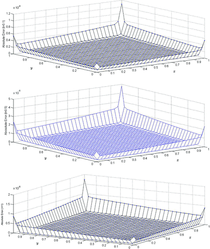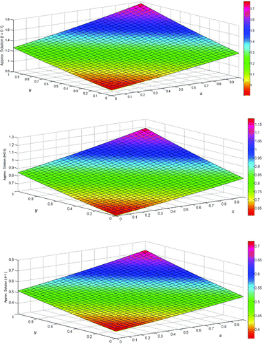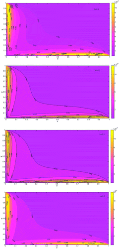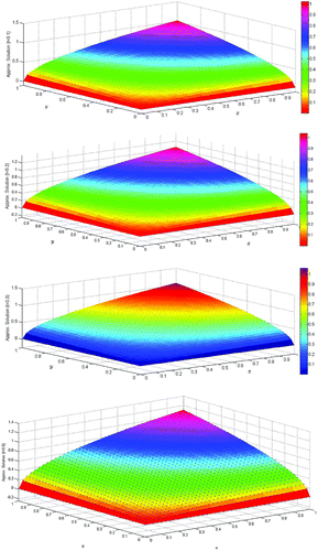The absolute errors in the BPM at different time levels $t\le 1$ is depicted in Figure 1, and the surface solution is depicted in Figure 2. Tables and Figure 1 confirms that our results are in good agreement with the results obtained in Cheng et al. (2014), Zhang et al. (2014) and exact solutions. The behavior of the solutions show the similar characteristics as depicted in Cheng et al. (2014), Zhang et al. (2014).

Example 2

We consider BPM (4) with the paramenters $h=1/96,\mathit{\alpha }=-1,\mathit{\beta }=1$ and $r=-48$ in the region $\mathbb{D}={[0,1]}^2$, subject to the initial condition:$$\begin{array}{c}\hfill {\mathit{\rho }}^0(\mathbf{x})=\frac{1}{4}\sqrt{2(x^2+y^2)+y+5},\forall \mathbf{x}\in \mathbb{D}\end{array}$$

while the boundary conditions are extracted from the exact solution$$\begin{array}{c}\hfill \mathit{\rho }(\mathbf{x},t)=\frac{1}{4}\sqrt{2(x^2+y^2)+y+\frac{t}{3}+5},(\mathbf{x},t)\in \mathbb{D}\times [0,T].\end{array}$$

The solutions are obtained for different values of $▵t$ and $h_x=h_y$. $L_2$ and $L\infty$ error norms at different time levels $t\le 1$ with $h_x=h_y=0.1$ and different time steps, are reported in Table 5, and $L_2$ and $L\infty$ error norms for $▵t=0.0001$ and different values of $h_x=h_y$ are reported in Table 6, while the $L_2$ and $L_{\infty }$ error norms for large time levels $5\le t\le 20$ are reported in Table 7. 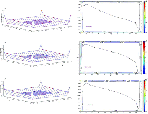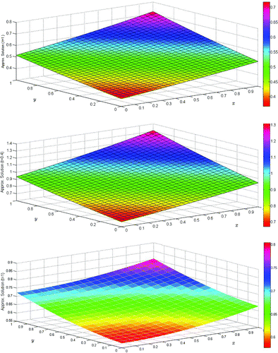The computational time in seconds, CPU(s), for different time intervals $t\le 20$ and various grid sizes with $▵t=0.0001$ is also reported in the above Tables 5–8. The contour and surface plots of absolute errors in the BPM at $t=0.1,0.5,1.0$ are depicted in Figure 3, and the surface solutions at these time intervals is depicted in Figure 4. It is evident that our results are in good agreement with the results obtained in Zhang et al. (2014) and exact solutions. Table 8 shows that the convergence quadratic. The behavior of $\mathit{\rho }(\mathbf{x},t)$ shows the similar characteristics as depicted in Zhang et al. (2014).

Example 3

We consider BPM (4) with the parameters $h=1/5,\mathit{\alpha }=1$ and $r=0$ in the region $\mathbb{D}={[0,1]}^2$, subject to the initial condition:$$\begin{array}{c}\hfill {\mathit{\rho }}^0(\mathbf{x})=\sqrt{xy},\forall \mathbf{x}\in \mathbb{D}\end{array}$$

while the boundary conditions are extracted from the exact solution$$\begin{array}{c}\hfill \mathit{\rho }(\mathbf{x},t)=e^{\frac{t}{5}}\sqrt{xy},(\mathbf{x},t)\in \mathbb{D}\times [0,T].\end{array}$$

The solutions are computed with $▵t=0.0001$. In Table 9, the computed results, for $h_x=h_y=1/13$, are compared with the recent results in Zhang et al. (2014) and the exact solutions. The $L_2$ and $L_{\infty }$ error norms for large time levels $2\le t\le 10$ are reported in Table 10. The computational time in seconds, CPU(s), for different time intervals $t\le 10$, and $h_x=h_y=1/12$ with $▵t=0.0001$ is also reported in the Tables 9 and 10. The contour plots of absolute errors in the BPM at $t=0.1,0.2,0.3,0.5$ are depicted in Figure 5, and the surface solutions at these time intervals is depicted in Figure 6. It is evident that our results are in good agreement with the results obtained in Zhang et al. (2014) and exact solutions. The behavior of for $\mathit{\rho }(\mathbf{x},t)$ shows the similar characteristics as depicted in Cheng et al. (2014), Zhang et al. (2014).

5. Conclusions

In the present paper, the MCB-DQM has been implemented for the numerical computation of 2D BPM. We present three test problems to confirm the efficiency and accuracy of the method for BPM, which shows that the the MCB-DQM solutions are in good agreement with that of obtained by the recent results using IEFGM by Zhang et al. (2014) and element free kp-Ritz method by Cheng et al. (2014).

Further, the scheme is tested for large time for the given problems which shows that the results obtained for large time levels are in good agreement with the exact solutions. It is found that the order of convergence of MCB-DQM for the solutions of BPM is quadratic.

Additional information

Funding

The author received no direct funding for this research.

Notes on contributors

Brajesh Kumar Singh

Brajesh Kumar Singh has completed PhD in Cryptography from Indian Institute of Technology Roorkee (2012). He worked as an assistant professor in the Department of Mathematics, Graphics Era Hill University, Dehradun INDIA from August 2012 to March 2015. Currently, he is working as an assistant professor in the Department of Applied Mathematics, Babasaheb Bhimrao Ambedkar University Lucknow India. His research interest in area of Applied Mathematics such as Discrete Mathematics, Numerical Analysis, Numerical Solutions to Partial Differential Equations, Mathematical Modeling, Computational Fluid Dynamics, Computational aspects in Physics, Biology and Finance, etc. He has published research papers in reputed international journals of mathematical and engineering sciences.

References

- Arafa, A. A., Rida, S. Z., & Mohamed, H. (2011). Homotopy analysis method for solving biological population model. Communications in Theoretical Physics, 56, 797–800.
- Aronson, D. G. (1986). The porous medium equation. Lecture Notes in Mathematics, 10, 12–24.
- Arora, G., Mittal, R. C., & Singh, B. K. (2014). Numerical solution of BBM-burger equation with quartic B-spline collocation method. Journal of Engineering Science and Technology, 3(Special Issue 1), 104–116.
- Arora, G., & Singh, B. K. (2013). Numerical solution of Burgers’ equation with modified cubic B-spline differential quadrature method. Applied Mathematics and Computation, 224, 166–177.
- Bear, J. (1972). Dynamics of fluids in porous media. New York, NY: American Elsevier.
- Bellman, R., Kashef, B. G., & Casti, J. (1972). Differential quadrature: A technique for the rapid solution of nonlinear differential equations. Journal of Computational Physics, 10, 40–52.
- Cheng, R. J., Zhang, L. W., & Liew, K. M. (2014). Modelling of bilological population problems using the element-free kp-Ritz method. Applied Mathematics and Computation, 227, 274–290.
- Dibnedetto, E. (1993). Degerate parabolic equations. New York, NY: Springer- Verleg.
- Giuggioli, L., & Kenkre, V. M. (2003). Analytic solutions of a nonlinear convective equation in population dynamics. Physica D, 183, 245–259.
- Gottlieb, S. (2005). On high order strong stability preserving RungeKutta and multi step time discretizations. Journal of Scientific Computing, 25, 105–128.
- Gurtin, M. E., & Maccamy, R. C. (1977). On the diffusion of biological population. Mathematical Biosciences, 33, 35–49.
- Gurney, W. S. C., & Nisbet, R. M. (1975). The regulation of inhomogeneous populations. Journal of Theoretical Biology, 52, 441–457.
- Jager, W., & Lu, Y. G. (1997). Global regularity of solutions for general degerate parabolic equations in 1D. Journal of Differential Equations, 140, 365–377.
- Korkmaz, A., & Dag, I. (2011). Shock wave simulations using sinc differential quadrature method. Engineering with Computers, 28, 654–674.
- Korkmaz, A., & Dag, I. (2013). Cubic B-spline differential quadrature methods and stability for Burgers’ equation, 30, 320–344.
- Liu, Y., Li, Z., & Zhang, Y. (2011). Homotopy perturbation method to fractional biological population equation. Fractional Differential Calculus, 1, 117–124.
- Lu, Y. G. (2000). H-order estimates of solutions of biological populations. Applied Mathematics Letters, 13, 123–126.
- Okubo, A. (1980). Diffusion and ecological problem, mathematical models, biomathematics 10. Berlin: Springer.
- Prenter, P. M. (1975). Splines and Variational Methods. New York, NY: Wiley.
- Quan, J. R., & Chang, C. T. (1989a). New insights in solving distributed system equations by the quadrature methods-I. Computers & Chemical Engineering, 13, 779–788.
- Quan, J. R., & Chang, C. T. (1989b). New insights in solving distributed system equations by the quadrature methods-II. Computers & Chemical Engineering, 13, 1017–1024.
- Roul, P. (2010). Application of homotopy perturbation method to biological population model. Applied Mathematics and Computation, 10, 1369–1378.
- Shakeri, F., & Dehghan, M. (2006). Numerical solution of a biological population model using He’s variational iteration method. Computers & Mathematics with Applications, 54, 1197–1209.
- Shivanian, E. (2013). Analysis of meshless local radial point interpolation (MLRPI) on a nonlinear partial integro-differential equation arising in population dynamics. Engineering Analysis with Boundary Elements, 37, 1693–1702.
- Shu, C. (2000). Differential quadrature and its application in engineering. Great Britain: Athenaeum Press.
- Shu, C., Chen, W., Xue, H., & Du, H. (2001). Numerical study of grid distribution effect on accuracy of DQ analysis of beams and plates by error estimation of derivative approximation. International Journal for Numerical Methods in Engineering, 51, 159–179.
- Shu, C., & Richards, B. E. (1992). Application of generalized differential quadrature to solve two dimensional incompressible Navier-Stokes equations. International Journal for Numerical Methods in Fluids, 15, 791–8.
- Singh, B. K., & Arora, G. (2014). A numerical scheme to solve Fisher-type reaction-diffusion equations. Nonlinear Studies/Mesa- Mathematics in Engineering, Science and Aerospace, 5(2), 153–164.
- Singh, B. K., Arora, G., & Singh, M. K. (2016). A numerical scheme for the generalized Burgers-Huxley equation. Journal of the Egyptian Mathematical Society. doi:10.1016/j.joems.2015.11.003
- Singh, B. K., & Bianca, C. (2016). A new numerical approach for the solutions of partial differential equations in three-dimensional space. Applied Mathematics & Information Sciences, 10(5), 1–10.
- Singh, B. K., & Kumar, P. (2016a). FRDTM for numerical simulation of multi-dimensional, time-fractional model of Navier-Stokes equation. Ain Shams Engineering Journa. doi:10.1016/j.asej.2016.04.009
- Singh, B. K., & Kumar, P. (2016b). Numerical computation for time-fractional gas dynamics equations by fractional reduced differential transforms method. Journal of Mathematics and System Science, 6, 248–259.
- Singh, B. K., & Kumar, P. (2016c). A novel approach for numerical computation of Burgers’ equation (1 + 1) and (2 + 1) dimension. Alexandria Engineering Journal. doi:10.1016/j.aej.2016.08.023
- Singh, B. K., & Srivastava, V. K. (2015). Approximate series solution of multi-dimensional, time fractional-order (heat-like) diffusion equations using FRDTM. Royal Society Open Sciences, 2, 140511. doi:10.1098/rsos.140511
- Spiteri, J. R., & Ruuth, S. J. (2002). A new class of optimal high-order strongstability-preserving time-stepping schemes. SIAM Journal on Numerical Analysis, 40, 469–491.
- Spiteri, J. R., & Ruuth, S. J. (2004). Downwinding in high-order strong-stability-preserving Runge-Kutta methods. SIAM Journal on Numerical Analysis, 42, 974–996.
- Srivastava, V. K., Kumar, S., Awasthi, M. K., & Singh, B. K. (2014). Two-dimensional time fractional-order biological population model and its analytical solution. Egyptian Journal of Basic and Applied Sciences, 1, 71–76.
- Srivastava, V. K., Mishra, N., Kumar, S., Singh, B. K., & Awasthi, M. K. (2014). Reduced differential transform method for solving (1+n)-dimensional Burgers’ equation. Egyptian Journal of Basic and Applied Sciences, 1, 115–119.
- Srivastava, V. K., & Singh, B. K. (2014). A Robust finite difference scheme for the numerical solutions of two dimensional time-dependent coupled nonlinear Burgers’ equations. International Journal of Applied Mathematics and Mechanics, 10, 28–39.
- Zhang, L. W., Deng, Y. J., & Liew, K. M. (2014). An improved element-free Galerkin method for numerical modelling of bilological population problems. Engineering Analysis with Boundary Elements, 40, 181–188.
- Zhong, H. (2004). Spline-based differential quadrature for fourth order equations and its application to Kirchhoff plates. Applied Mathematical Modelling, 28, 353–366.