A novel approach toward coordinated inventory management of an agile multi-echelon multi-product supply chain

Abstract

Inventory control systems development is one of the most appealing issues of the supply chain management which have recently been studied by academicians and practitioners. In this paper, an inventory management framework and deterministic cost models within the context of this framework are structured for effective supply chain (SC) in an agile environment. To do so, we propose a three-echelon multi-product SC including multiple suppliers, multiple manufacturing firms, and multiple retailers. Moreover, a fuzzy-ANP framework is employed to evaluate suppliers’ agility level and to elicit suitable suppliers aiming at achieving an agile network. To develop operational measures of SC flexibility, a cost structure is defined which captures some different operational cost factors including inventory holding, backordering, lost sell, and ordering costs. Furthermore, a hybrid metaheuristic algorithm is developed to tackle the computational complexity of a production-inventory planning task. Finally, numerical experiments validate the proposed solution methodology.

Keywords:

• inventory management
• multi-echelon multi-product inventory models
• agile supply chain
• fuzzy analytic network process
• differential evolution algorithm
• particle swarm optimization

Public Interest Statement

This paper attempts to solve the inventory management problem of a supply chain. The considered supply chain includes two layers of the manufacturers and retailers. It is challenging to manage inventory orders and cycles in both layers of the supply chain simultaneously and in accordance with each other. In this regard, an integrated mathematical program is developed. The developed model consists of three sub-models each of which attempts to cope with the inventory system of the retailer, warehouse of the manufacturer, and production of the manufacturer. Since the proposed model is not computationally solvable, a metaheuristic algorithm is developed to solve the proposed integrated model.

1. Introduction

Supply chain management (SCM) as an emerging field has recently attracted industrial community. SCM is implemented in order to manage multiple relationships across the supply chain (SC) with respect to the entire flow of information, materials, and services to fulfill customer demand in an efficient manner. This philosophy led to fundamental changes in the field of business management (Li & Wang, 2007). In this regard, commodities should be produced and distributed at the right quantities, to the right locations, and at the right time resulting in minimization of the entire costs of system wide (Routroy & Kodali, 2005).

Beside diverse decisions involved in the field of SCM, SC inventory management is one of the major challenges of SCM. While, researchers and industrial practitioners have recently devoted major attention to develop inventory problems in SCM by considering a whole SC as a network of procurement, transformation, and delivering firms (Routroy & Kodali, 2005). Some of the important reasons of efficient inventory management in SC operations could be declared as follows. First, 20–60% of the total assets of manufacturing firms belong to inventory (Gümüs & Güneri, 2007). Second, there are various forms of inventories throughout the SC including raw materials, semi-finished or finished goods, as well as in-process between locations. Third, holding of inventories can cost anywhere between 20 and 40% of their value (Ganeshan & Harrison, 1995). More importantly, lack of comprehensive inventory management throughout the SC can lead to the bullwhip effect as well as, excessive inventory investments, lost revenues, misguided capacity plans, ineffective transportation, missed production schedules, and poor customer service (Giannoccaro, Pontrandolfo, & Scozzi, 2003). On the other hand, traditional SC was a sequence of weakly connected activities both within and outside of the organization, whose most important results are capacity-infeasible plans with unbalanced inventories and poor overall performance (Torabi & Hassini, 2009). Inventory replenishment decisions are made taking into account only those cost parameters that could be directly influenced by the planning company. An optimal solution is concluded for only a single company. Hence, based on traditional inventory management, optimality is not guaranteed when multiple companies or a whole SC are taken into consideration (Glock, 2012). Tackling with this lack of coordination is a spread era for SC managers (Torabi & Hassini, 2009). So, having multi-echelon inventory management applied to continue competitive and reduce inventory, operation costs are decreased and customer service is improved (Gümüs & Güneri, 2007).

In this regards, the classic square root economic-order quantity (EOQ) model developed by Harris is one of the earliest models to cover two basic questions that any inventory control system has to answer when and how much to order in every basic textbook on operations research/management science, operations management, and SCM (Pentico & Drake, 2009). Next, the basic EOQ model has been extended to as the economic production quantity (EPQ) or economic manufacturing quantity (EMQ) model. In the extension, the replenishment order is assumed to be received at a constant finite rate over time against EOQ which is instantaneous replenishment (Pentico, Drake, & Toews, 2009).

In this study, we attempt to cope with the shortcomings of the traditional inventory management. Hence, this paper deals with the inventory management of SCs. In this regard, an inventory management framework is proposed to satisfy customers’ needs in a three-echelon SC in an agile manner. The supposed SC consists of multi-supplier, multi-retailer, and multi-manufacturing plant which offers multiple product types to the customers. Upon the proposed inventory management framework, different levels of the supposed network are integrated to decrease total production-inventory costs of the SC. In order to achieve a more flexible and responsible network, manufacturing firms purchase raw materials from variant suppliers, and assemble them into final products, then the final products are split and delivered to the retailers. Moreover, a fuzzy-ANP framework is proposed to evaluate suppliers’ agility levels in responding to the downward firms’ needs.

Rest of the paper is structured as follows. Section 2 briefly reviews the previously conducted researches. Section 3 presents the proposed three-echelon multi-item SC structure. The models of the proposed inventory policies as well. And the proposed solution methodology is described thoroughly in Section 4. This paper follows in Section 5 on computational experiments to validate the proposed model. Finally, some conclusions and future research directions are provided in the last section.

2. Literature review

Since numerous researchers addressed different aspects of the multi-echelon inventory system and the integrated SC, we provide only the studies which have been recently published in order to conclude contributions of this paper in comparison with the body of literature. Additionally, literature body of agile SCs is briefly reviewed in this section.

2.1. The multi-echelon inventory system

A multi-echelon inventory system is a system in which an item reaches to the final customer after moving more than one stage (Rau, Wu, & Wee, 2003). The problems related to the multi-echelon inventory control have been perused since 1950s. The main aim of these problems is to control the inventory levels by determining the size of the orders for each echelon during each period so that objective function is optimized (Zhou, Chen, & Ge, 2012). The first research toward the two-echelon inventory model dates back to the one by Clark and Scarf (1960). In their study, the optimality of a base stock policy for the pure serial inventory system was demonstrated and an efficient decomposing method was introduced in order to compute the optimal base stock ordering policy. In another seminal work, Sherbrooke (1968 cited by Rau et al., 2003) introduced an ordering policy of two-echelon inventory model for warehouse and retailer while pure shortage was allowed at the retailers. Moreover, Mitra (2009) and Hill, Seifbarghy, and Smith (2007) presented single-item, two-echelon inventory models applying continuous review. In addition to the two-level systems, abundant researches have been presented on multi-echelon inventory control. Routroy and Kodali (2005) developed a single product, three-echelon inventory planning model. They applied the differential evolution algorithm to minimize the total system-wide cost by determining ordering/production quantity and inventory/service level. Two other instances of multi-item, multi-echelon systems are modeled by Caggiano, Jackson, Muckstadt, and Rappold (2009) and Yang and Lin (2010).

2.2. The integrated SC

Another interesting issue related to SCM is to optimize SC integrated systems. In particular, the integrated inventory replenishment decisions between buyer and vendor are called the joint economic lot sizing problem (JELP) upon which order, production, and shipment quantities are determined from the perspective of the SC with the objective of minimizing total system costs (Ben-Daya, As’ad, & Seliaman, 2010). Goyal (1976) was the first who introduced the idea of joint total cost for the buyer and the supplier. Thereafter, numerous researches have been appeared to coordinate inventory replenishment decisions among individual companies to benefit the entire supply network. Sajadieh and Akbari Jokar (2009) developed a model in which demand at the buyer followed a linear demand function. In Sawik’s (2009) study, supplier operates multiple production lines in parallel and supplies multiple products to a manufacturer. And, the manufacturer runs a production facility with multiple stages in series. In the case of more than two actors in an integrated inventory model, Joglekar and Tharthare (1990) were the first who modeled a system with a single-vendor and multiple identical buyers (SVMB). Chan and Kingsman (2007) developed Banerjee and Burton’s model (1994), in which a basic cycle time was considered for the vendor and the order interval of each buyer was assumed to be an integer multiple of the basic cycle. Hoque (2008) developed a single-manufacturer multi-buyer integrated inventory SC applying close relationship between the actors of the SC for a costless way of benefit sharing. The case of multi-vendor in the integrated inventory models was analyzed by Chen and Sarker (2010), who studied a buyer sourcing a product from multiple vendors supposing a single truck to collect the products from the vendors in a milk run. The authors modeled a freight cost function which considers both product weights and travel distances.

With respect to the multi-echelon inventory models, Banerjee, Kim, and Burton (2007) offered a common delivery cycle in order to reduce the complexity of the problem. The first research toward three stages SC with one or more firms at each stage was introduced by Khouja (2003) whose considered system comprised of a single raw material supplier, multiple manufacturers, and multiple buyers, which was further extended by Ben-Daya and Al-Nassar (2008). Finally, some papers took into account more cost factors in multi-echelon inventory models, such as deteriorating inventory models by Yang and Wee (2000) and stochastic demand arrivals by Zhou et al. (2012).

2.3. Agile SC

The concept of the agile SC has been taken into account as means of achieving a competitive edge in rapidly changing business environments. In this regard, one of the most important issues is supplier selection. According to the related body of literature, supplier selection process comprises of three main steps: criteria formulation, qualification, and choice. The last stage involves selecting suitable partners through qualified partners for specific purchases with respect to the criteria which are related to the suppliers’ level of agility (Wu & Barnes, 2011).In the context of agility, as the capability of a process to respond to unanticipated changes, the first research toward agility measurement dates back to the one by Dove (1994 cited by Sherehiy, Karwowski, & Layer, 2007). An integrated agility index which was defined as combination of agile capabilities intensity levels has been applied by some authors such as Tsourveloudis & Valavanis, 2002. Moreover, the linguistic expressions and fuzzy logic were augmented to overcome the uncertainty and ambiguity of the agility indicators and definitions (Lin, Chiu, & Tseng, 2006; Tsourveloudis & Valavanis, 2002).

In order to evaluate agility level of suppliers, numerous research papers have been published so far, among which Tam and Tummala (2001) presented an AHP-based model to select a vendor for a telecommunications system applying some criteria with respect to cost, technical, and operational factors. Moreover, the developed models have been equipped with fuzzy set theory in order to cope with the involved fuzziness in the problem, as Mikhailov (2002) which developed a fuzzy-AHP model to tackle supplier selection in an ambiguous environment. In addition to AHP, ANP has been another method used in this field, since it compensate a great drawback of AHP. ANP is capable to model interrelations among decision criteria and alternatives. Similar to many applications of ANP, this method has been adopted in the field of agile supplier selection as in Büyüközkan and Çifçi (2011) and Sarkis, Talluri, and Gunasekaran (2007).

With respect to the literature, no attention has been dedicated to multi-item, multi-vendor, multi-buyer SC in an agile environment. Hence, this paper is devoted to inventory management by developing EOQ and EPQ models subject to stockouts in a three-echelon SC for the first time. The proposed SC embraces multi-supplier, multi-manufacturer, and multi-retailer, while SC’s agility is enhanced by assessing suppliers with respect to the agility criteria.

3. Proposed multi-echelon SC

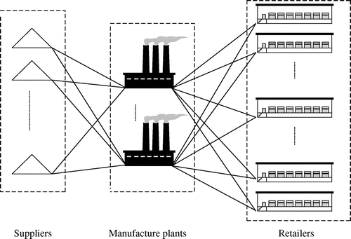
The present study attempts to develop an inventory management framework in which decisions on inventory control system are made in a multi-item, multi-buyer, multi-vendor, multi-echelon SC. This framework is developed to seek when and how much product should be placed as an order/production with respect to the related inventory policy. To do so, a three-echelon SC including various manufacturing plants with capacitated storage, multiple retailers at the bottom level, and multiple suppliers at the top level is proposed. In this regard, it is supposed several manufacturing firms operate based upon multi-product production system.

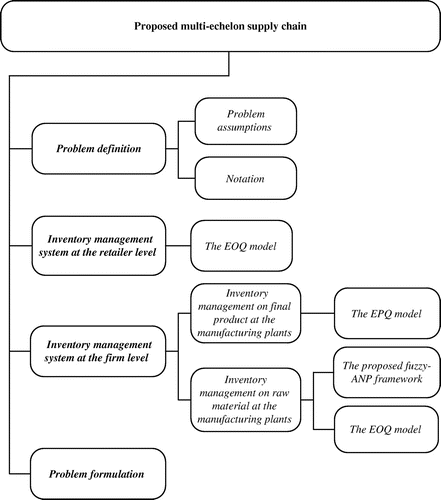
As illustrated in Figure 1, each stage in the SC is fed from upper echelon and feed lower ones. The entire customers’ demand is firstly entered into the retailers so that is responded through retailers’ on-hand inventory. And, retailers’ needs are forwarded to manufacturing plants to be produced in an economic manner. To do so, multiple manufacturing firms are considered to supply retailers’ demands leading to a more flexible and responsible network. In addition, manufacturing firms’ requirements are fulfilled through various suppliers, and are delivered in economic batch size assuring agility in terms of flexibility and performance. In other words, the supposed network suggests multiple product types which are produced at different costs at various manufacturing plants to the customers arrived to the retailer nodes. Furthermore, the connections between two partners have been suggested in subsequent levels allowing physical transportation and information relationships between entities for the sake of the product flow efficiency and effectiveness. This section elaborates the proposed model including components depicted in Figure 2.

Figure 1. A three-echelon supply chain.

Figure 2. General schema of Section 3.

3.1. Problem definition

In order to manage inventory system corresponding to retailer level, a deterministic EOQ policy with partial backordering is supposed. Also, relevant inventory control system of manufacturing firms is analyzed applying two inventory policies including EOQ and EPQ from which an EOQ policy with pure backordering is implemented to investigate the inventory system of raw material as well as an EPQ policy with pure backordering for the final products. In this regard, the problem is defined so as to minimize total cost of the corresponding SC.

3.1.1. Problem assumptions

Assumptions of the problem as followings:

• Customer demand rates for all products are deterministic and constant during the planning period;

• Production rates of all products are deterministic and constant;

• Production rate is greater than demand rate for every product in the SC;

• Replenishment lead times for retailers and firms are zero;

• Replenishment batch sizes for retailers and manufacturing plants are equal;

• Raw material warehouses of manufacturing plants have finite capacity;

• Shortage is allowed; and

• Shortage, ordering, and holding costs at each level are known.

3.1.2. Notations

The proposed EOQ and EPQ models are dedicated to determine how much and when product should be placed as an order and a production. In this regard, the used notations are as followings:

Indices
i	=	Index for final products (i = 1, …, N);
i′	=	Index for raw materials (i′ = 1, …, n);
j	=	Index for retailer nodes (j = 1, …, nr);
k	=	Index for manufacturing plant nodes (k = 1, …, nm);
z	=	Index for supplier nodes (z = 1, …, ns);

Parameters
$D_{ij}^r$	=	Demand per year for final product i at retailer j;
$P_{ik}^m$	=	Production rate per year for final product i at manufacturing plant k;
srij	=	The unit selling price of final product i at retailer j;
${Co}_{ij}^r$	=	The fixed cost of placing an order for final product i at retailer j;
${Co}_{ik}^m$	=	The fixed cost of receiving an order for final product i at manufacturing plant k;
${Co}_{i^{\prime }k}^m$	=	The fixed cost of placing an order for raw material i′ at manufacturing plant k;
${Cpu}_{ij}^r$	=	The variable cost of purchasing a unit of final product i at retailer j;
${Ch}_{ij}^r$	=	The cost to hold a unit of final product i at retailer j in inventory for a cycle;
${Ch}_{ik}^m$	=	The cost to hold a unit of final product i at manufacturing plant k in inventory for a cycle;
${Ch}_{i^{\prime }k}^m$	=	The cost to hold a unit of raw material i′ at manufacturing plant k in inventory for a cycle;
${Cb}_{ij}^r$	=	The cost to keep a unit backordered of final product i at retailer j for a cycle;
${Cb}_{ik}^m$	=	The cost to keep a unit backordered of final product i at manufacturing plant k for a cycle;
${Cb}_{i^{\prime }k}^m$	=	The cost to keep a unit backordered of raw material i′ at manufacturing plant k for a cycle;
${Cg}_{ij}^r$	=	The goodwill loss on a unit of unfilled product i demand at retailer j;
${Cl}_{ij}^r$	=	The cost for a lost sale of final product i at retailer j, including the lost profit on that unit and any goodwill loss (${sr}_{ij}-{Cpu}_{ij}^r+{Cg}_{ij}^r$);
fi′k	=	Space occupied by each unit of raw material i′ at manufacturing plant k;
fk	=	Available warehouse space for all raw materials at manufacturing plant k;
qi′kz	=	The percentage of order quantity of raw material i′ from manufacturing plant k toward supplier z (i.e. $0\le q_{i^{\prime }kz}\le 1$);
ccii′k	=	The consumption coefficient of final product i from raw material i′ at manufacturing plant k;
${\mathit{\beta }}_{ijk}^r$	=	The fraction of stockouts of final product i at retailer j from manufacturing plant k that will be backordered

Decision variables
$D_{ik}^m$	=	Demand per year for final product i at manufacturing plant k;
$D_{i^{\prime }k}^m$	=	Demand per year for raw material i′ at manufacturing plant k;
$Q_{ijk}^r$	=	The order quantity for final product i at retailer j toward manufacturing plant k;
$Q_{ik}^m$	=	The production quantity for final product i at manufacturing plant k;
$Q_{i^{\prime }kz}^m$	=	The order quantity for raw material i′ at manufacturing plant k toward supplier z;
qijk	=	The percentage of order quantity of final product i from retailer j toward manufacturing plant k (i.e. $0\le q_{ijk}\le 1$);
$x_{i{i}^{\prime }k}^{}$	=	1 if ${cc}_{i{i}^{\prime }z}\ge 0$, otherwise 0;
$T_{ij}^r$	=	The time between orders or the length of an order cycle of final product i at retailer j;
$T_{ik}^m$	=	The time between productions or the length of a planning cycle of final product i at manufacturing plant k;
$T_{i^{\prime }k}^m$	=	The time between orders or the length of an order cycle of raw material i′ at manufacturing plant k;
$K_{ijk}^r$	=	The integer multiple of the length of order cycle of final product i at retailer j from manufacturing plant k;
$K_{ik}^m$	=	The integer multiple of the length of production cycle of final product i at manufacturing plant k;
$F_{ijk}^r$	=	The fill rate or the percentage of demands for final product i at retailer j from manufacturing plant k that will be filled from stock;
$F_{ik}^m$	=	The fill rate or the percentage of demands for final product i at manufacturing plant k that will be filled from stock;
$F_{i^{\prime }kz}^m$	=	The fill rate or the percentage of demands for raw material i′ at manufacturing plant k from supplier z that will be filled from stock;
${TC}_{EOQ}^r$	=	Total cost per year for the retailers;
${TC}_{EOQ}^m$	=	Total related cost to EOQ per year for the manufacturing plants;
${TC}_{EPQ}^m$	=	Total related cost to EPQ per year for the manufacturing plants;
TCm	=	Total cost per year for the manufacturing plants (i.e. ${TC}^m={TC}_{EOQ}^m+{TC}_{EPQ}^m$);
TC	=	Total cost per year for the whole of the SC

3.2. Inventory management system at the retailer level

In this study, retailer level is proposed to offer N types of product to the customers. Customer demands are provided through on-hand inventory of the retailers and their orders are partially backordered in the case of shortage. There are several manufacturing firms in the SC to supply retailers in order to enhance flexibility and agility of the network because each retailer places an order for the final products toward variant manufacturing plants. While, the length of order cycle of each final product at each retailer is multiple of each other. And, the order quantity of any product i placed in every cycle of time is equal. However, the order quantity placed by a retailer may vary from one retailer to the others. To do so, the retailer-level proposed model is described in this section.

3.2.1. The EOQ model

According to the previous researches on inventory management frameworks, there are six basic decision variables to develop EOQ model with partial backordering: Q (the order quantity), T (the length of an order cycle), I (the maximum inventory level), S (the maximum stockout level), B (the maximum backordered position), and F (the fill rate or the percentage of demand). However, it is adequate to find two variables among the six above, hence, the remainder might be calculated. Therefore, $T_{ij}^r$, the length of an order cycle of product i at retailer j, and $F_{ijk}^r$, the fraction of demand for final product i at retailer j from manufacturing plant k to be filled from stock, and integer value of the multiplier of the order cycles ($K_{ijk}^r$) are supposed as decision variables. In order to develop operational measures of retailer level’s flexibility, an objective function which captures some different operational cost factors such as inventory holding, backordering, ordering, and goodwill loss is defined.

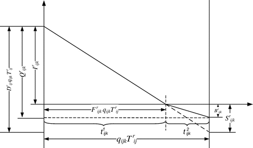
Partial backordering is supposed for customers who face unavailable production inventory at the retailer level. It must be noted, the backordering rate of each product at each retailer from each firm is assumed a constant rate, which $0\le {\mathit{\beta }}_{ijk}^r\le 1$). Figure 3 illustrates the inventory level of EOQ problem with partial backordering for final product i at retailer j from firm k.

Figure 3. Inventory level of EOQ problem with partial backordering.

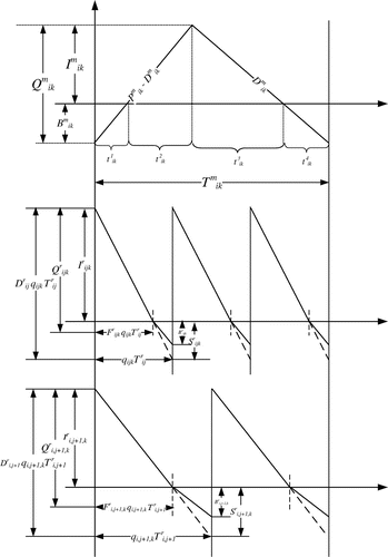
As depicted in Figure 3, order cycle for final product i at retailer j from manufacturing plant k is divided into two sub-interval including $t_{ijk}^1$ which is demand time with $t_{ijk}^1=F_{ijk}^r{q}_{ijk}{T}_{ij}^r$, and $t_{ijk}^2$ which is shortage time with $t_{ijk}^2=\left(1-F_{ijk}^r\right)q_{ijk}{T}_{ij}^r$. Therefore, based upon these values, $I_{ijk}^r$ is the maximum inventory level of final product i at retailer j from manufacturing plant k with $I_{ijk}^r=D_{ij}^r{t}_{ijk}^1=D_{ij}^r{F}_{ijk}^r{q}_{ijk}{T}_{ij}^r$, $S_{ijk}^r$ is the maximum stockout quantity of product i at retailer j from manufacturing plant k with $S_{ijk}^r=D_{ij}^r{t}_{ijk}^2=D_{ij}^r\left(1-F_{ijk}^r\right)q_{ijk}{T}_{ij}^r$, $B_{ijk}^r$ is the maximum backorder position of product i at retailer j from manufacturing plant k with $B_{ijk}^r={\mathit{\beta }}_{ijk}^r{S}_{ijk}^r={\mathit{\beta }}_{ijk}^r{D}_{ij}^r\left(1-F_{ijk}^r\right)q_{ijk}{T}_{ij}^r$. With respect to these expressions, order quantity of each product at each retailer node from each manufacturing plant is calculable using Equation 1. Hence, the relevant average profit of retailer level per year (i.e. Average profit per year = income − [(ordering + purchasing + inventory holding + backordering + goodwill loss) cost])) is maximized through Equation 2 and the constraints are taken into account (Equation 3).(1) $$Q_{ijk}^r=I_{ijk}^r+B_{ijk}^r=D_{ij}^r{F}_{ijk}^r{q}_{ijk}{T}_{ij}^r+{\mathit{\beta }}_{ijk}^r{D}_{ij}^r(1-F_{ijk}^r)q_{ijk}{T}_{ij}^r$$(1) (2) $$\begin{array}{c}max\mathrm{\Pi }\left(T_{ij}^r,F_{ijk}^r,q_{ijk},K_{ijk}^r\right)=\left[{\sum }_i{\sum }_j{\sum }_k{sr}_{ij}{D}_{ij}^r\left[F_{ijk}^r+{\mathit{\beta }}_{ijk}^r\left(1-F_{ijk}^r\right)\right]\right]\hfill \\ -\left[\begin{array}{c}\sum _i\sum _j\sum _k\frac{{Co}_{ij}^r}{q_{ijk}{T}_{ij}^r}+\sum _i\sum _j\sum _k{Cpu}_{ij}^r{q}_{ijk}{D}_{ij}^r\left[F_{ijk}^r+{\mathit{\beta }}_{ijk}^r\left(1-F_{ijk}^r\right)\right]\hfill \\ +\sum _i\sum _j\sum _k\frac{C{h}_{ij}^r{D}_{ij}^r{q}_{ijk}{T}_{ij}^r{F}_{ijk}^{r^2}}{2}\hfill \\ +\sum _i\sum _j\sum _k\frac{{\mathit{\beta }}_{ijk}^r{Cb}_{ij}^r{D}_{ij}^r{q}_{ijk}{T}_{ij}^r{\left(1-F_{ijk}^r\right)}^2}{2}+\sum _i\sum _j\sum _k{Cg}_{ij}^r{D}_{ij}^r\left(1-{\mathit{\beta }}_{ijk}^r\right)\left(1-F_{ijk}^r\right)\hfill \end{array}\right]\hfill \end{array}$$(2) (3) $$K_{ijk}^r{q}_{ijk}{T}_{ij}^r=K_{i,j+l,k}^r{q}_{i,j+l,k}{T}_{i,j+l}^r\begin{array}{cc}& \begin{array}{cc}\forall & i,k,j,l=1,...,nr-j\end{array}\end{array}$$(3)

The value of the order quantity, the maximum inventory level, and the maximum backorder position of product i at retailer j are, respectively, yield as follows:

$Q_{ij}^r=\sum _k{Q}_{ijk}^r$; $I_{ij}^r=\sum _k{I}_{ijk}^r$; $B_{ij}^r=\sum _k{B}_{ijk}^r$

As shown in Appendix A, $\mathrm{\Pi }\left(T_{ij}^r,F_{ijk}^r,q_{ijk},K_{ijk}^r\right)$ is maximized by the $T_{ij}^r,F_{ijk}^r,q_{ijk},K_{ijk}^r$ that minimizes the average cost per year, as illustrated in Equation 4.(4) $$\begin{array}{c}\begin{array}{cc}Min& \end{array}{TC}_{EOQ}^r(T_{ij}^r,F_{ijk}^r,q_{ijk},K_{ijk}^r)=\sum _i\sum _j(\sum _k\frac{{Co}_{ij}^r}{q_{ijk}{T}_{ij}^r}+\\ \frac{{Ch}_{ij}^r{D}_{ij}^r{q}_{ijk}{T}_{ij}^r{F}_{ijk}^{r^2}}{2}+\frac{{\mathit{\beta }}_{ijk}^r{Cb}_{ij}^r{D}_{ij}^r{q}_{ijk}{T}_{ij}^r{(1-F_{ijk}^r)}^2}{2}+\\ {Cl}_{ij}^r{D}_{ij}^r(1-{\mathit{\beta }}_{ijk}^r)(1-F_{ijk}^r))\end{array}$$(4)

3.3. Inventory management system at the firm level

As mentioned earlier, the proposed SC offers N types of products to the customers based upon a coordinated mechanism among suppliers, manufacturing firms, and retailers. In the considered SC of the proposed model, a manufacturing firm is supplied from its suppliers (upper level) and processes the raw materials to the final products. Therefore, two inventory control policies including EOQ and EPQ are simultaneously modeled to analyze the related inventory system to the manufacturing plants. A comprehensive description of the supposed inventory control policies is presented in the next sub-sections.

3.3.1. Inventory management on final products at the manufacturing plants

In order to model the inventory system of the final products at the manufacturing plants, an EPQ model with complete backordering is adopted in which the plants have constant production rate $P_{ik}^m$ and demand rate $D_{ik}^m$ ($P_{ik}^m>D_{ik}^m$). 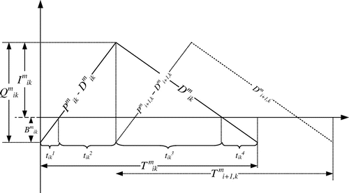Having the manufacturing plant inventory system analyzed, $T_{ik}^m$, the length of an planning cycle of product i at manufacturing plant k, and $F_{ik}^m$, the fraction of demand for final product i at manufacturing plant k to be filled from stock, and $K_{ik}^m$, the integer multiple of the length of production cycle of final product i at manufacturing plant k are obtained in such away to minimize total inventory system costs. So, holding costs, ordering, and backordering costs of the finished products are modeled as objective function. As depicted in Figure 4, manufacturing plant k produces $Q_{ik}^m$ of final product i during production cycle $T_{ik}^m$ upon EPQ model with full backordering. In this model, the economic quantity of each finished product may vary from a firm to another one.

Figure 4. Inventory level of EPQ model with full backordering.

The length of planning cycle of each final product at each firm is divided into four intervals including production/demand time, demand time, and shortage time as elaborated in Figure 4 for which $t_{ik}^1=\left(1-F_{ik}^m\right)T_{ik}^m\raisebox{1ex}{$D_{ik}^m$}\!\left/ \!\raisebox{-1ex}{$P_{ik}^m$}\right.$; $t_{ik}^2=F_{ik}^m{T}_{ik}^m\raisebox{1ex}{$D_{ik}^m$}\!\left/ \!\raisebox{-1ex}{$P_{ik}^m$}\right.$; $t_{ik}^3=F_{ik}^m{T}_{ik}^m\left(1-\raisebox{1ex}{$D_{ik}^m$}\!\left/ \!\raisebox{-1ex}{$P_{ik}^m$}\right.\right)$; $t_{ik}^4=\left(1-F_{ik}^m\right)T_{ik}^m\left(1-\raisebox{1ex}{$D_{ik}^m$}\!\left/ \!\raisebox{-1ex}{$P_{ik}^m$}\right.\right)$.

With respect to the above values, the value of the maximum inventory level, the maximum backorder position, the production quantity of final product i at manufacturing plant k, and total costs of this model are found applying Equations 5–8, respectively. In addition, Equation 9 is extended to compute the relationship between the production cycles of final products at each firm which are multiple of each other.(5) $$I_{ik}^m=\left(P_{ik}^m-D_{ik}^m\right)t_{ik}^2=F_{ik}^m{T}_{ik}^m{D}_{ik}^m\left(1-\raisebox{1ex}{$D_{ik}^m$}\!\left/ \!\raisebox{-1ex}{$P_{ik}^m$}\right.\right)$$(5) (6) $$B_{ik}^m=D_{ik}^m{t}_{ik}^4=\left(1-F_{ik}^m\right)T_{ik}^m{D}_{ik}^m\left(1-\raisebox{1ex}{$D_{ik}^m$}\!\left/ \!\raisebox{-1ex}{$P_{ik}^m$}\right.\right)$$(6) (7) $$\begin{array}{c}{Q}_{ik}^m=I_{ik}^m+B_{ik}^m=F_{ik}^m{T}_{ik}^m{D}_{ik}^m\left(1-\raisebox{1ex}{$D_{ik}^m$}\!\left/ \!\raisebox{-1ex}{$P_{ik}^m$}\right.\right)+\\ \left(1-F_{ik}^m\right)T_{ik}^m{D}_{ik}^m\left(1-\raisebox{1ex}{$D_{ik}^m$}\!\left/ \!\raisebox{-1ex}{$P_{ik}^m$}\right.\right)\end{array}$$(7) (8) $$\begin{array}{c}{\begin{array}{cc}Min& \end{array}TC}_{EPQ}^m\left(T_{ik}^m,F_{ik}^m\right)=\sum _i\sum _k\frac{{Co}_{ik}^m}{T_{ik}^m}+\sum _i\sum _k\left(\frac{{Ch}_{ik}^m{D}_{ik}^m{T}_{ik}^m{F}_{ik}^{m^2}}{2}\right)\left(1-\raisebox{1ex}{$D_{ik}^m$}\!\left/ \!\raisebox{-1ex}{$P_{ik}^m$}\right.\right)\\ +\sum _i\sum _k\left(\frac{{Cb}_{ik}^m{D}_{ik}^m{T}_{ik}^m{\left(1-F_{ik}^m\right)}^2}{2}\right)\left(1-\raisebox{1ex}{$D_{ik}^m$}\!\left/ \!\raisebox{-1ex}{$P_{ik}^m$}\right.\right)\end{array}$$(8) (9) $$\begin{array}{c}{K}_{ik}^m{x}_{i{i}^{\prime }k}{T}_{ik}^m\raisebox{1ex}{$D_{ik}^m$}\!\left/ \!\raisebox{-1ex}{$P_{ik}^m$}\right.=K_{i+l,k}^m{x}_{i+l,i^{\prime },k}{T}_{i+l,k}^m\raisebox{1ex}{$D_{i+l,k}^m$}\!\left/ \!\raisebox{-1ex}{$P_{i+l,k}^m$}\right.\\ \begin{array}{cc}& \begin{array}{cc}\forall & i^{\prime },k,i,l=1,...,N-i\end{array};\end{array}\begin{array}{cc}& x_{i{i}^{\prime }k}\ne 0\end{array}\end{array}$$(9)

3.3.2. Inventory management on raw materials at the manufacturing plants

As mentioned earlier, various suppliers provide manufacturing plants demands in order to enhance flexibility and responsibility in the turbulent and rapidly changing market. In this regard, suppliers’ agility levels are assessed to elicit suitable suppliers applying a fuzzy-ANP framework which is developed according to the relevant criteria of agile SCs.

3.3.2.1. The proposed fuzzy-ANP framework

In the supposed network, raw materials which are consumed in producing the final products at firms are provided by variant suppliers so that the network flexibility is obtained. In order to achieve a more flexible and responsible SC, supplier’s agility level is investigated applying analytic network process (ANP), leading to elicit agile suppliers. In this regard, an ANP framework is developed to assess suppliers’ agility level. Since most of the decisions made in diverse contexts are driven upon expert preferences, fuzzy sets theory is utilized to overcome the uncertainty and ambiguity of the preference-based comparisons of decision-makers as well.

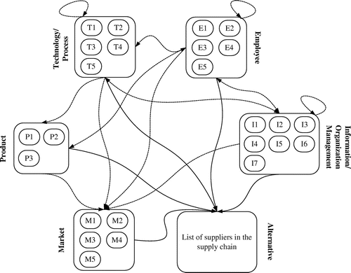
For the sake of brevity, description of the developed the proposed fuzzy-ANP model is skipped and the readers are referred to Rafiei and Rabbani (2011). Additionally, decision criteria are adopted from the agility context with respect to the agile supplier’s characteristics (Christian et al., 2001; Lin et al., 2006; Sharifi & Zhang, 1999; Tsourveloudis &Valavanis, 2002). In this regard, decision criteria and their corresponding clusters are listed in Table 1, where the network structure of the proposed ANP model is shown in Figure 5.

Table 1. Agility measurement factors

Cluster	Criteria	Code
Technology/process	Manufacturing speed	T1
	Products design and manufacture flexibility	T2
	Operations efficiency and effectiveness (leanness)	T3
	Appropriate/new technology (hard and soft)	T4
	Skill and knowledge enhancing technologies	T5
	IT skills and knowledge	T6
Product	Product flexibility	P1
	Product/services quality	P2
	Product volume flexibility	P3
Market	Products and services delivery quickness and timelines	M1
	Customer-driven innovations	M2
	Production support, production, supply & distribution, and new product introduction responsiveness	M3
	Inventory turnover	M4
	Customer satisfaction	M5
Employee	Multi-skilled and flexible people	E1
	Employee skills utilization	E2
	Continuous training and development	E3
	Learning organization	E4
	Employee satisfaction	E5
Information/organization management	Networking	I1
	Perfect degree of enterprise information system	I2
	Information network extensiveness	I3
	Information accessible to Beneficiary	I4
	Change management	I5
	The degree of cooperation with other enterprises	I6
	Concurrent execution of activities	I7

Figure 5. ANP network to rank suppliers.

Having the proposed fuzzy-ANP model implemented to assess suppliers’ agility level, the related value to the alternatives’ (suppliers) agility is concluded. The obtained values are normalized to the weights, q_i′kz. In this regard, q_i′kz is introduced as the percentage of order quantity of each raw material at each manufacturing plant which is provided through each supplier. Since q_i′kz = the value of supplier’s agility level/∑supplier the value of supplier’s agility level, then $0\le q_{i^{\prime }kz}\le 1$, and ${\sum }_k{q}_{i^{\prime }kz}=1$; hence, the order quantity for raw materials at the firms is split and forwarded to different suppliers upon the calculated weights ($Q_{i^{\prime }kz}^m=q_{i^{\prime }kz}{Q}_{i^{\prime }k}^m$). Based upon this method, firms’ demand could be satisfied rapidly from different suppliers.

3.3.2.2. The EOQ model

The EOQ model with complete backordering considers each manufacturing plant with a constant demand rate $D_{i^{\prime }k}^m$ (i′ = 1, …, n; k = 1, …, nm). The proposed manufacturing plants have finite capacity to store raw materials. Based on the supposed EOQ policy, manufacturing plant k places an order for raw material i′ to supplier z. Although, the order quantities placed by firms might vary from one firm to another, the order quantity of any raw material i′ at any manufacturer k is assumed equal. In this regard, this section is developed to seek the length of an order cycle of raw material i′ at manufacturing plant k; $T_{i^{\prime }k}^m$ and the fill rate or of demands for raw material i′ at manufacturing plant k from supplier z that will be filled from stock; $F_{i^{\prime }kz}^m$ due to minimize the corresponding inventory system costs. To do so, the summation of holding costs, ordering and backordering costs of raw materials is assumed as objective function. Additionally, it is assumed the length of order cycle of each raw material at each firm is an integer multiple of the length of production cycle of the final products which consume that raw material.

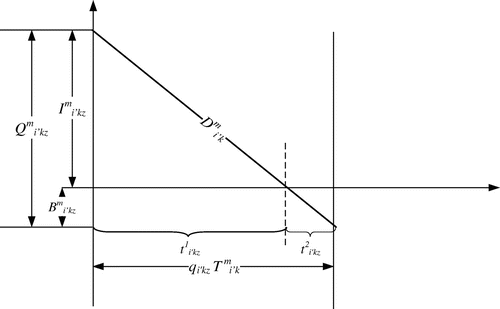
Figure 6 illustrates the inventory level of EOQ problem with complete backordering for raw material i′ at manufacturing plant k from supplier z. As shown in Figure 6, the summation of the demand time and the shortage time corresponds to the length of an order cycle of raw material i′ at manufacturing plant k from supplier z (i.e. $q_{i^{\prime }kz}{T}_{i^{\prime }k}^m=t_{i^{\prime }kz}^1+t_{i^{\prime }kz}^2$), where $t_{i^{\prime }kz}^1=F_{i^{\prime }kz}^m{q}_{i^{\prime }kz}{T}_{i^{\prime }k}^m$; $t_{i^{\prime }kz}^2=\left(1-F_{i^{\prime }kz}^m\right)q_{i^{\prime }kz}{T}_{i^{\prime }k}^m$.

Figure 6. The inventory level of EOQ problem with full backordering for at the firm level.

As depicted in Figure 6, $I_{i^{\prime }kz}^m$ is the maximum inventory level of raw material i′ at manufacturing plant k from supplier z with $I_{i^{\prime }kz}^m=D_{i^{\prime }k}^m{F}_{i^{\prime }kz}^m{q}_{i^{\prime }kz}{T}_{i^{\prime }k}^m$, $S_{i^{\prime }kz}^m$ is the maximum stockout quantity of raw material i′ at manufacturer k from supplier z with $S_{i^{\prime }kz}^m=D_{i^{\prime }k}^m\left(1-F_{i^{\prime }kz}^m\right)q_{i^{\prime }kz}{T}_{i^{\prime }k}^m$, $B_{i^{\prime }kz}^m$ is the maximum backorder position of raw material i′ at manufacturer k from supplier z with $B_{i^{\prime }kz}^m=S_{i^{\prime }kz}^m=D_{i^{\prime }k}^m\left(1-F_{i^{\prime }kz}^m\right)q_{i^{\prime }kz}{T}_{i^{\prime }k}^m$. The EOQ model with complete backordering is a particular case of EOQ model with partial backordering in which the backordering rate of product that will be backordered equals one. Further, the order quantity of each product at each firm from each supplier is yield applying Equation 10 with respect to the values of $I_{i^{\prime }kz}^m$ and $B_{i^{\prime }kz}^m$.(10) $$Q_{i^{\prime }kz}^m=D_{i^{\prime }k}^m{F}_{i^{\prime }kz}^m{q}_{i^{\prime }kz}{T}_{i^{\prime }k}^m+D_{i^{\prime }k}^m\left(1-F_{i^{\prime }kz}^m\right)q_{i^{\prime }kz}{T}_{i^{\prime }k}^m$$(10)

The order quantity, the maximum inventory level, and the maximum backorder position of raw material i′ at manufacturer k could be found using $Q_{i^{\prime }k}^m={\sum }_z{Q}_{i^{\prime }kz}^m$; $I_{i^{\prime }k}^m={\sum }_z{I}_{i^{\prime }kz}^m$; $B_{i^{\prime }k}^m={\sum }_z{B}_{i^{\prime }kz}^m$.

Based on Equation 11, the average cost of manufacturing plants’ inventory under EOQ policy per year is obtained.(11) $$\begin{array}{c}\begin{array}{cc}Min& \end{array}{TC}_{EOQ}^m\left(T_{i^{\prime }k}^m,F_{i^{\prime }kz}^m\right)=\sum _{i^{\prime }}\sum _k\sum _z\frac{{Co}_{i^{\prime }k}^m}{q_{i^{\prime }kz}{T}_{i^{\prime }k}^m}\\ +\sum _{i^{\prime }}\sum _k\sum _z\frac{{Ch}_{i^{\prime }k}^m{D}_{i^{\prime }k}^m{q}_{i^{\prime }kz}{T}_{i^{\prime }k}^m{F}_{i^{\prime }kz}^{m^2}}{2}+\sum _{i^{\prime }}\sum _k\sum _z\frac{{Cb}_{i^{\prime }k}^m{D}_{i^{\prime }k}^m{q}_{i^{\prime }kz}{T}_{i^{\prime }k}^m{\left(1-F_{i^{\prime }kz}^m\right)}^2}{2}\end{array}$$(11)

3.4. Problem formation

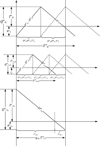
As mentioned earlier, it was supposed the order interval of each final product at each retailer is an integer multiple of each other. Also, length of the production cycle of final products at each manufacturing plant is assumed to be an integer multiple of each other. Having the various inventory policies integrated for the sake of total SC cost reduction, some relationships between different levels of the network are taken into consideration. The characteristics at the upper levels have a relationship with the lower level ones. These associations comprise of relation between the value of order and planning cycle, demand, and shortage of final products as well as raw materials. Figures 7 and 8 illustrate the relationships among the order/planning cycle at retailer and firm levels, and order/production cycle at firm level, respectively.

Figure 7. The combined inventory profile for the level of the retailer and manufacturing plant.

Figure 8. The combined inventory profile for the level of manufacturing plant.

In this regard, mathematical model in Equations 13–20 is proposed.(12) $$minTC={TC}_{EOQ}^r+T{C}_{EOQ}^m+T{C}_{EPQ}^m$$(12)

s.t:(13) $$\sum _{i^{\prime }=1}^N{f}_{i^{\prime }k}{D}_{i^{\prime }k}^m{T}_{i^{\prime }k}^m\le f_k\begin{array}{cc}& \begin{array}{ccc}& \forall & k\end{array}\end{array}$$(13) (14) $$D_{ik}^m=\sum _{j=1}^{nr}{q}_{ijk}{D}_{ij}^r;\forall i,k$$(14) (15) $$D_{i^{\prime }k}^m=\sum _{i=1}^N{cc}_{i{i}^{\prime }k}{D}_{ik}^m;\forall i^{\prime },k$$(15) (16) $$T_{ik}^m=K_{ijk}^r{q}_{ijk}{T}_{ij}^r=K_{i,j+l,k}^r{q}_{i,j+l,k}{T}_{i,j+l}^r\begin{array}{cc}& \begin{array}{cc}\forall & i,k,j,l=1,...,nr-j\end{array}\end{array}$$(16) (17) $$\begin{array}{c}{T}_{i^{\prime }k}^m=K_{ik}^m{x}_{i{i}^{\prime }k}{T}_{ik}^m{D}_{ik}^m/P_{ik}^m=K_{i+l,k}^m{x}_{i+l,i^{\prime },k}{T}_{i+l,k}^m{D}_{i+l,k}^m/P_{i+l,k}^m\\ \forall i^{\prime },k,i,l=1,\dots ,N-i;x_{i{i}^{\prime }k}\ne 0\end{array}$$(17) (18a) $$B_{ik}^m=max\left\{\left[B_{i^{\prime }k}^m\times c{c}_{i{i}^{\prime }k}/\sum _{i}c{c}_{i{i}^{\prime }k}\right];\forall i^{\prime }\right\};\forall i,k$$(18a) (18b) $$\begin{array}{c}\left(1-F_{ik}^m\right)T_{ik}^m{D}_{ik}^m\left(1-\raisebox{1ex}{$D_{ik}^m$}\!\left/ \!\raisebox{-1ex}{$P_{ik}^m$}\right.\right)=\\ max\left\{\left.\left[\left(\sum _z{D}_{i^{\prime }k}^m\left(1-F_{i^{\prime }kz}^m\right)q_{i^{\prime }kz}{T}_{i^{\prime }k}^m\right)\times \raisebox{1ex}{${cc}_{i{i}^{\prime }k}$}\!\left/ \!\raisebox{-1ex}{${\sum }_i{cc}_{i{i}^{\prime }k}$}\right.\right];\forall i^{\prime }\right\}\right.;\forall i,k\end{array}$$(18b) (19a) $$B_{ij}^r=\sum _{k=1}^{nm}{q}_{ijk}{B}_{ik}^m;\forall i,j$$(19a) (19b) $$\begin{array}{c}\sum _{k=1}^{nm}{\mathit{\beta }}_{ijk}^r{D}_{ij}^r\left(1-F_{ijk}^r\right)q_{ijk}{T}_{ij}^r=\sum _{k=1}^{nm}{q}_{ijk}\left(1-F_{ik}^m\right)T_{ik}^m{D}_{ik}^m\left(1-\raisebox{1ex}{$D_{ik}^m$}\!\left/ \!\raisebox{-1ex}{$P_{ik}^m$}\right.\right)\\ \begin{array}{cc}& \forall i,j\end{array}\end{array}$$(19b) (20) $$\begin{array}{c}{T}_{ij}^r,{T_{ik}^m,T}_{i^{\prime }k}^m,q_{ijk},q_{i^{\prime }kz},F_{ijk}^r,F_{i^{\prime }kz}^m,F_{ik}^m\in \left[0,1\right];\begin{array}{cc}& D_{i^{\prime }k}^m{D}_{ik}^m,TC>0;\end{array}\\ K_{ijk}^r,K_{ik}^m>0\begin{array}{cc}& \begin{array}{cc}\text{and}& \text{integer}\end{array}\end{array};\begin{array}{cc}& x_{i{i}^{\prime }k}=0,1;\forall i,i^{\prime },j,k,z\end{array}\end{array}$$(20)

In the proposed model, the objective function seeks to minimize total average cost of SC per year given in Equation 12. As mentioned earlier, Constraints Equation 13 is devoted to meet the warehouse capacity limitation at the firms. As shown in Equations 14 and 15, demand rate of final products at the retailer stage influences on the demand rate of final products as well as raw material at the firm stage. Equation 16 expresses the length of planning cycle of each final product at each firm is assumed to be an integer multiple of the order interval of final product at each retailer from the firm. Equation 17 shows the associations between the relevant order and production cycles of the manufacturing firms. Based upon Equation17, the length of order cycle of each raw material at each firm is an integer multiple of the length of production cycle of the final products which consume that raw material. Since, all raw materials are used with different consumption coefficients in producing the finished product. Hence, deficiency on final products at manufacturing plant level and retailer level depends on the shortage of raw materials as shown in Equations 18 and 19, respectively. Finally, Equation 20 demonstrates the real and integer variables.

4. Solution methodology

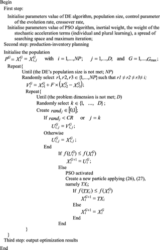
This section is developed in order to provide a proper methodology to tackle the computational complexity of the problem. To do so, a hybrid metaheuristic algorithm including a differential evolution (DE) algorithm and a particle swarm optimization (PSO) algorithm is applied. The algorithm starts through DE with random initial population up to the selection step where the current population is compared with its corresponding trial vector based on their objective function values. If the trial vector satisfies the conditions given by Equation 25, then it is copied to the next generation; otherwise, it creates a new solution by conducting the PSO phase. Having the PSO phase implemented, a perturbation is created in the population, leading to maintain the diversity of the population as well as to reach a good optimal solution. In advanced, the pseudo-code of the hybrid optimization algorithm is briefly presented in Figure 9.

Figure 9. Pseudo-code of the applied hybrid optimization algorithm.

4.1. Differential evolution algorithm

DE was firstly introduced by Storn and Price in 1995 as a powerful heuristic method for solving non-linear, non-differentiable, and multi-modal optimization problems. This technique has been structured based upon a combination of simple arithmetic operators, the classical crossover, mutation, and selection operators. In this method, the purpose of mutation and crossover is to generate new vectors, and the vectors will survive to the next generation are determined upon selection operator (Damak, Jarboui, Siarry, & Loukil, 2009).

Broad scope and applicability of DE have been challenged in diverse disciplines, such as digital filter design, batch fermentation process, dynamic optimization of continuous polymer reactor, optimization of heat exchangers, optimization of non- linear functions, fuzzy decision-making problems of fuel ethanol production, and multi sensor fusion. (Routroy & Kodali, 2005). Moreover, Falcone, Lopes, and Coelho (2008) have highly recommended DE for the SC optimization problem as well as for other logistics-related problems due to its robustness. Advantages of DE such as a simple structure, ease of use, a great robustness, and a fast convergence lead to promote its reputation in many fields (Damak et al., 2009; Routroy & Kodali, 2005). A brief description of the developed DE strategy is elaborated as followings:

4.1.1. Population structure

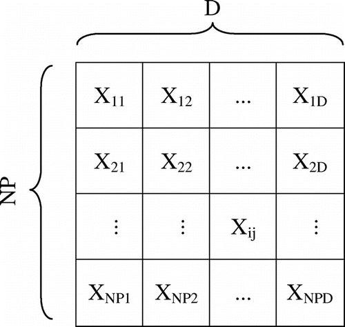
DE starts with randomly generated X^G_i (i = 1, ..., NP) vector to create the initial population, where the index i represents the ith solution of population, and G denotes the current generation. Supposing the index j indicates the jth element in the solution vector which contains D elements. In addition, NP indicates the population size. The initial population and the vectors that belong to it are, respectively, represented as follows:(21) $$P^G{=X}_i^G\begin{array}{ccc}& \text{with}& i=1,...,NP\end{array}$$(21) (22) $$X_i^G=X_{i,j}^G\begin{array}{ccc}& \text{with}& \begin{array}{ccc}j=1,...,D;& \text{and}& G=1,...,G_{max}\end{array}\end{array}$$(22)

As shown in Figure 10, the initial population of the DE algorithm can be represented as a string of element as people.

Figure 10. The general schematic of the population in DE.

The population size as a main factor of the DE has a significant role in the algorithm convergence speed. Whereas too small size leads to insufficient exploration, on contrary, too large size leads to increase the number of function evolutions upon which the algorithm convergence speed is negatively affected.

4.1.2. Mutation

After initialization of the population, mutation operator starts with selecting three vectors {X_r1, X_r2, X_r3} randomly in the population set of NP elements such that r1 ≠ r2 ≠ r3 ≠ i. The selected vectors are combined to create a mutant vector as depicted in Equation 23 in which F is the control parameter of the evolution rate such that F ϵ [0, 1].(23) $$V_i^G=X_{r1}^G+F\times \left(X_{r2}^G-X_{r3}^G\right);i=1,...,NP,r1,r2,r3\in \{1,...,NP\}$$(23)

4.1.3. Crossover

Once the mutant vector is generated, crossover operator attempts to create a trial vector applying the following equation:(24) $$U_{i,j}^G=\left\{\begin{array}{c}{V}_{i,j}^G\begin{array}{cc}\begin{array}{cc}\hfill & \end{array}\hfill & \text{if}\begin{array}{cc}\hfill & \end{array}{rand}_j\le \end{array}CR\begin{array}{cc};& j=k\end{array}\hfill \\ X_{i,j}^G\begin{array}{cc}\begin{array}{cc}\hfill & \end{array}\hfill & \text{otherwise}\end{array}\hfill \end{array}\right.$$(24)

where $j=1,\dots ,D,$ $k\in \{1,\dots ,D\}$ indicates the random parameter’s index, chosen once for each i. $CR\in \left[0,1\right]$ is the crossover factor upon which the crossover of various elements is executed. And, r and j are uniform random numbers which are compared with value of the crossover rate to determine the element of the trial vector. If the value of the random number is less or equal to crossover rate, the trial element is copied from the mutant vector; otherwise, it is selected from the current vector.

4.1.4. Selection

The selection step is performed by comparing the current population with its corresponding trial vector based on their objective function values. As shown in Equation 25, if the objective function value of the trial vector is less than the current population’s one, it takes place in the next generation; otherwise, the PSO algorithm is activated.(25) $$X_i^{G+1}=\left\{\begin{array}{c}{U}_i^G\begin{array}{cc}\begin{array}{cc}& \begin{array}{cc}& \end{array}\end{array}\hfill & \text{if}\begin{array}{cc}\hfill & f(U_i^G)\end{array}\le \end{array}f(X_i^G)\hfill \\ \text{PSO}\begin{array}{cc}\begin{array}{cc}\text{activated}\hfill & \end{array}\hfill & \text{otherwise}\end{array}\hfill \end{array}\right.$$(25)

As a result, all solutions of the next generation are as good as or better than the current population. Once the current generation is updated, mutation, crossover, and selection operators are repeated until the optimum, or the predefined termination criterion is met.

4.2. Particle swarm optimization

The presented PSO by Kennedy and Eberhart (1995) is an evolutionary calculations technique. The mechanism of PSO has been driven from the simulation of social behavior of flying birds which exchange their information to solve optimization problems. The PSO’s solution is a set of particle in the position of search space. Each particle maintains information on itself experience as well as other particles’ ones upon which moves toward the best point in the search space. To do so, two basic equations including velocity vector and position vector have been introduced as follows:(26) $$V_i(t+1)=w{V}_i(t)+c_1{r}_1\left(x_{ibest}(t)-x_i(t)\right)+c_2{r}_2\left(x_{gbest}(t)-x_i(t)\right)$$(26) (27) $$x_i(t+1)=x_i(t)+V_i(t+1)$$(27)

The velocity vector comprises of three parts; the first part refers to the inertia of the previous velocity. The second part, namely, cognition component, presents the personal thinking of the particle. And, the third one, namely, social component, presents the cooperation among the particles. $V_i(t)$ and $x_i(t)$indicate the velocity and the position of ith particle in tth iteration, respectively. $x_{ibest}$ and $x_{gbest}$ represent the best previous position of each particle, and the best position among all the particles in the swarm, respectively. w as the inertial weight has a role of balancing the global exploration and the local exploitation abilities of the swarm. c1 and c2 represent the weight of the stochastic acceleration terms, and r1 and r2 as the random functions in order to search the space in a better manner.

5. Numerical experiments

This section is developed to show validity of the proposed methodology tackling complexity of the proposed model. To do so, several instances in different sizes are extended. Table 2 corresponds to the generated problems in which different numbers of final products, raw materials, retailers, manufacturing firms, and suppliers are considered. The numerical data of the final products and raw materials at each level of the SC are a modified version from the ones given in Pasandideh, Niaki, and Nia (2011). The related data of problem 4 are only presented in Tables 3–5 for the sake of brevity. The initial values of the DE parameters including the crossover factor (CR), the control parameter of the evolution rate (F), and the population size (NP) are chosen to be 0.6, 0.7, and 20 by testing the problem, respectively. It is noted that the capability and the convergence speed of the proposed methodology lead to coverage the solution to the near optimal point after 30 iterations even for high iteration than 30. Then, in order to reduce the time of problem-solving, iteration factor is considered 30 in report.

Table 2. The relevant data of the instances size

Index problem No.	i	i′	j	k	z
1	2	3	2	2	2
2	2	3	4	3	3
3	3	5	4	3	3
4	5	5	4	3	5
5	5	5	4	4	5

Table 3. Relevant date of final products at the retailer’s level

Final prod.	Retailer No.
	1					2					3					4
	D^rij	Co^rij	Ch^rij	Cb^rij	Cl^rij	D^rij	Co^rij	Ch^rij	Cb^rij	Cl^rij	D^rij	Co^rij	Ch^rij	Cb^rij	Cl^rij	D^rij	Co^rij	Ch^rij	Cb^rij	Cl^rij
1	420	1	5	3	10	240	2	4	4	8	480	3	6	8	5	510	5	2	3	6
2	160	2	9	4	8	380	1	8	5	9	390	2	5	3	9	430	4	3	8	10
3	340	4	7	2	6	120	4	9	3	5	530	1	3	9	2	280	3	6	4	6
4	180	1	8	6	4	410	3	5	4	6	230	5	7	5	4	390	1	4	6	7
5	230	6	3	1	8	180	2	6	9	7	480	4	8	2	3	320	2	8	5	8

Table 4. Relevant data of final product at the manufacturing plant’s level

Final product	Manufacturing No.
	1				2				3
	P^mik	Co^mik	Ch^mik	Cb^mik	P^mik	Co^mik	Ch^mik	Cb^mik	P^mik	Co^mik	Ch^mik	Cb^mik
1	2300	3	5	2	2000	2	3	6	1950	5	9	4
2	1900	4	8	4	2050	1	8	4	1850	3	4	3
3	2050	2	1	5	2300	4	7	5	2040	3	5	8
4	1590	5	4	6	1600	3	4	3	1650	4	3	4
5	2250	2	6	1	2100	2	2	6	2300	1	6	7

Table 5. Relevant data of raw material at the manufacturing plant’s level.

Raw material No.	Manufacturing plant No.												Final product No.
	1				2				3				1	2	3	4	5
	Co^mi′k	Ch^mi′k	Cb^mi′k	fi′k	Co^mi′k	Ch^mi′k	Cb^mi′k	fi′k	Co^mi′k	Ch^mi′k	Cb^mi′k	fi′k	ccii′	ccii′	ccii′	ccii′	ccii′
1	2	5	5	2	1	8	5	2	5	3	7	2	2	3	1	2	4
2	4	7	7	2	5	8	6	2	3	5	3	2	3	5	0	4	2
3	6	8	9	4	3	1	3	4	3	6	4	4		0	3	1	2
4	1	5	4	3	2	2	5	3	4	9	2	3	4	1	1	2	0
5	2	6	2	1	5	3	2	1	2	7	5	1	0	0	3	0	2

Notes: f_k = 14000; for all manufacturing plants, f_i′1 = f_i′2 = … = f_i′k = f_i′, cc_ii′1 = cc_ii′2 = … = cc_ii′k = cc_ii′.

And, the initial values of PSO parameters are selected as follows: the inertial weight is calculated according to $w=\mathit{\chi }=2/\left(\mathit{\phi }-2+\sqrt{{\mathit{\phi }}^2-4\mathit{\phi }}\right)$ in the first iteration, where φ = φ₁ + φ₂, φ₁ and φ₂are similarly selected as 2.05; and gradually reduced by Equation 28, in which wdamp is supposed to be 0.99. Moreover, the weight of the stochastic acceleration terms are obtained applying c₁ = 0.001φ₁χ, and c₂ = 0.001φ₂χ. It is noted that the algorithm is stopped after 30 iterations.(28) $$w=w\times wdamp$$(28)

5.1. Numerical sample of the proposed fuzzy-ANP framework

As mentioned in Section 3, the weights of order quantity for raw materials at manufacturing plants from each supplier are determined applying the proposed fuzzy-ANP framework. In this section, we implement the proposed structure only for problem 5 to demonstrate the application of the proposed ANP framework. In this regard, five manufacturing companies/suppliers are considered as alternatives. For instance, Tables 6 and 7 demonstrate the relevant judgments about alternatives with respect to criterion Product flexibility and the clusters with respect to cluster Technology/Process-related, respectively; the weights of comparison matrices are obtained as: 0.244, 0.166, 0.093, 0.063, and 0.435 for alternatives 1, 2, 3, 4, and 5, respectively. With respect to data in Table 7, the resulted weights are 0.362, 0.062, 0.044, 0.150, 0.106, and 0.276 for technology/process related, product related, market related, employee related, and information/organization management related, respectively. After performing the developed model and with respect to the results obtained in limit supermatrix, final weights W = (0.0537, 0.0240, 0.0094, 0.0074, 0.0631) × 10⁻³ are calculated.

Table 6. Judgment about alternatives with respect to criteria product flexibility

	A1	A2	A3	A4	A5
A1	(1, 1, 1)	(1, 5/2, 4)	(2, 4, 6)	(3, 5, 7)	(1/4, 5/8, 1)
A2	(1/4, 5/8, 1)	(1, 1, 1)	(1, 5/2, 4)	(2, 4, 6)	(1/6, 1/3, 1/2)
A3	(1/6, 1/3, 1/2)	(1/4, 5/8, 1)	(1, 1, 1)	(1, 5/2, 4)	(1/7, 5/21, 1/3)
A4	(1/7, 5/21, 1/3)	(1/6, 1/3, 1/2)	(1/4, 5/8, 1)	(1, 1, 1)	(1/8, 3/16, 1/4)
A5	(1, 5/2, 4)	(2, 4, 6)	(3, 5, 7)	(4, 6, 8)	(1, 1, 1)

Table 7. Judgment about clusters with respect to cluster technology/process related

	T	P	M	E	I	A
T	(1, 1, 1)	(4, 6, 8)	(5, 7, 9)	(2, 4, 6)	(3, 5, 7)	(1, 5/2, 4)
P	(1/8, 3/16, 1/4)	(1, 1, 1)	(1, 5/2, 4)	(1/6, 1/3, 1/2)	(1/4, 5/8, 1)	(1/7, 5/21, 1/3)
M	(1/9, 7/45, 1/5)	(1/4, 5/8, 1)	(1, 1, 1)	(1/7, 5/21, 1/3)	(1/6, 1/3, 1/2)	(1/8, 3/16, 1/4)
E	(1/6, 1/3, 1/2)	(2, 4, 6)	(3, 5, 7)	(1, 1, 1)	(1, 5/2, 4)	(1/4, 5/8, 1)
I	(1/7, 5/21, 1/3)	(1, 5/2, 4)	(2, 4, 6)	(1/4, 5/8, 1)	(1, 1, 1)	(1/6, 1/3, 1/2)
A	(1/4, 5/8, 1)	(3, 5, 7)	(4, 6, 8)	(1, 5/2, 4)	(2, 4, 6)	(1, 1, 1)

5.2. Computational results

The applied DE-PSO algorithm is coded in Matlab 7.8.0 (R2009a) software and run on a PC with 4.00 GB RAM and 2.00 Ghz processor. The results of objective function and elapsed time for the problem instances are summarized in Table 8. Each test problem has been run 15 times and the minimum objective function value along with its corresponding solutions is reported.

Table 8. The value of objective functions and CPU time

	Problem No.
	1	2	3	4	5
OFV	2602.4523	8607.4667	18378.9515	35538.3804	45438.0066
CPU time	2.60	7.45	9.33	14.72	19.75

It must be noted that the supposed problem has also been evaluated applying the classic DE algorithm. And then, the proposed solution is applied to enhance the solution methodology performance. The results of the objective function for the problem instances which are solved by the DE algorithm are shown in Table 9, and compared with the results of Table 8. As shown in Table 9, in the most problems, the objective function values resulted upon the DE–PSO algorithm is yield less than the one, which are presented applying the classic DE algorithm.

Table 9. The comparison results of objective function value applying the DE and DE–PSO algorithms

	Problem No.
	1	2	3	4	5
OFV-DE	2891.4194	9347.0349	17978.6103	39942.5499	50617.3324
OFV-DE-PSO	2602.4523	8607.4667	18378.9515	35538.3804	45438.0066

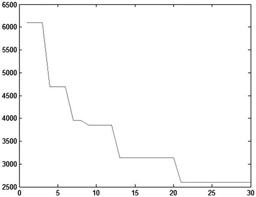
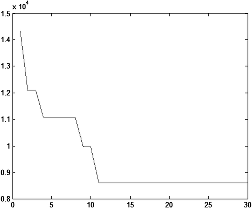
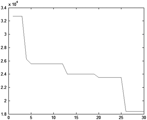
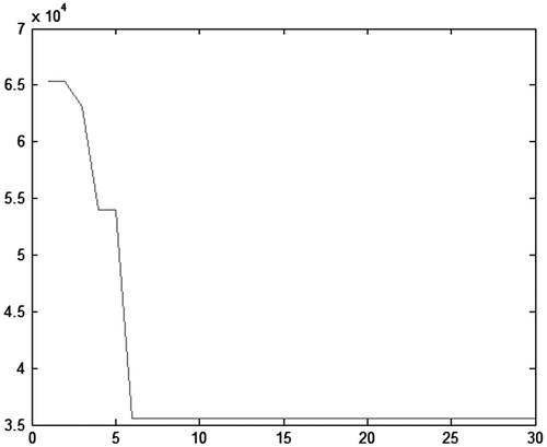
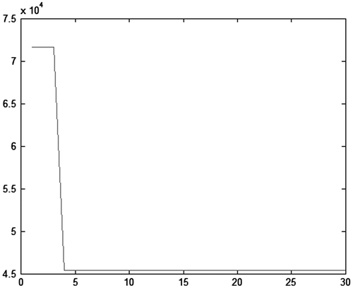
Moreover, we evaluate the convergence rate of the developed algorithm in order to obtain a solution for all five considered problems. In this regard, the convergence trend of these solutions for each problem 1–5 is demonstrated in Figures 11^{Figure 12Figure 13Figure 14}–15, respectively. These figures illustrate capability of the DE–PSO algorithm in reaching a good solution in its early iterations as well as the reduction in the convergence speed by increasing the problem size.

Figure 11. The convergence path (problem 1).

Figure 12. The convergence path (problem 2).

Figure 13. The convergence path (problem 3).

Figure 14. The convergence path (problem 4).

Figure 15. The convergence path (problem 5).

6. Conclusion and future research directions

This paper addressed a novel inventory management framework for a three-echelon multi-item SC having multiple suppliers, multiple manufacturing plants, and multiple retailers. In this regard, several inventory control policies corresponding to various levels have been proposed in an integrated point of view, leading to achieving the optimization of global SC. Moreover, in order to increase network flexibility and agility, different actors at each echelon were supposed to provide the lower levels’ demands. To do so, a fuzzy-ANP model was developed to assess suppliers and elicit the suitable ones upon their agility level. Additionally, a mixed-integer non-linear mathematical model was proposed in order to coped with the inventory management problem. The proposed model was solved applying a hybrid DE–PSO algorithm to tackle the computational complexity of the problem.

To extend current direction of this paper, some suggestions are provided. First, other assumptions could be considered in SC to make it more practical, such as other kinds of inventory control policy, e.g. fixed/linear lead time, time costs. Second, modeling SC uncertainty could make it more realistic. Third, it is highly recommended to define other decision criteria in agile SCs, and other types of fuzzy numbers and preference methods, such as the eigenvalue method, the logarithmic least squares method, and the weighted least squares method, to determine the related weights of elements of pairwise comparison matrices and analyze them to elicit the best one. Lastly, developing other metaheuristics and heuristics to tackle complexity of the integrated inventory model is suggested.

Additional information

Funding

Funding. The authors received no direct funding for this research.

Notes on contributors

Maryam Alimardani

Maryam Alimardani graduated from the School of Industrial Engineering, University of Tehran. She has published several papers in international scholarly journals and conference proceedings in the field of production planning, inventory control, and enterprise resource planning..

Hamed Rafiei

Hamed Rafiei obtained his PhD from School of Industrial Engineering, University of Tehran. He received his BSc and MSc degrees of Industrial Engineering from University of Tehran as an honored student. His research interests include applications of operations research in operations management on which he has published several papers in international journals and conference proceedings.

Masoud Rabbani

Masoud Rabbani is a professor of Industrial Engineering at School of Industrial Engineering, University of Tehran. He has published more than 50 papers in international journals, e.g. European Journal of Operational Research, International Journal of Production Research, International Journal of Production Economics. His current research interests comprise production planning, applied graph theory, productivity management, and EFQM.

Appendix A

Developing Equation 4 from Equation 2

$$\begin{array}{c}\begin{array}{cc}max& \mathrm{\Pi }\left(T_{ij}^r,F_{ijk}^r,q_{ijk},K_{ijk}^r\right)\end{array}=\left[\sum _i\sum _j\sum _k{sr}_{ij}{D}_{ij}^r\left[F_{ijk}^r+{\mathit{\beta }}_{ijk}^r\left(1-F_{ijk}^r\right)\right]\right]-\hfill \\ \left[\begin{array}{c}\sum _i\sum _j\sum _k\frac{{Co}_{ij}^r}{q_{ijk}{T}_{ij}^r}+\sum _i\sum _j\sum _k{Cpu}_{ij}^r{q}_{ijk}{D}_{ij}^r\left[F_{ijk}^r+{\mathit{\beta }}_{ijk}^r\left(1-F_{ijk}^r\right)\right]+\hfill \\ \sum _i\sum _j\sum _k\frac{{Ch}_{ij}^r{D}_{ij}^r{q}_{ijk}{T}_{ij}^r{F}_{ijk}^{r^2}}{2}+\sum _i\sum _j\sum _k\frac{{\mathit{\beta }}_{ijk}^r{Cb}_{ij}^r{D}_{ij}^r{q}_{ijk}{T}_{ij}^r{\left(1-F_{ijk}^r\right)}^2}{2}+\sum _i\sum _j\sum _k{Cg}_{ij}^r{D}_{ij}^r\left(1-{\mathit{\beta }}_{ijk}^r\right)\left(1-F_{ijk}^r\right)\hfill \end{array}\right]\hfill \end{array}$$$$\begin{array}{c}=\sum _i\sum _j\sum _k{D}_{ij}^r\left({sr}_{ij}-{Cpu}_{ij}^r{q}_{ijk}\right)\left[F_{ijk}^r+{\mathit{\beta }}_{ijk}^r\left(1-F_{ijk}^r\right)\right]-\\ \left[\begin{array}{c}\sum _i\sum _j\sum _k\frac{{Co}_{ij}^r}{q_{ijk}{T}_{ij}^r}+\sum _i\sum _j\sum _k\frac{{Ch}_{ij}^r{D}_{ij}^r{q}_{ijk}{T}_{ij}^r{F}_{ijk}^{r^2}}{2}+\sum _i\sum _j\sum _k\frac{{\mathit{\beta }}_{ijk}^r{Cb}_{ij}^r{D}_{ij}^r{q}_{ijk}{T}_{ij}^r{\left(1-F_{ijk}^r\right)}^2}{2}\\ +\sum _i\sum _j\sum _k{Cg}_{ij}^r{D}_{ij}^r\left(1-{\mathit{\beta }}_{ijk}^r\right)\left(1-F_{ijk}^r\right)\end{array}\right]\end{array}$$$$\begin{array}{c}=\sum _i\sum _j\sum _k{D}_{ij}^r\left({sr}_{ij}-{Cpu}_{ij}^r{q}_{ijk}\right)\left[1-\left(1-{\mathit{\beta }}_{ijk}^r\right)\left(1-F_{ijk}^r\right)\right]-\\ \left[\begin{array}{c}\sum _i\sum _j\sum _k\frac{{Co}_{ij}^r}{q_{ijk}{T}_{ij}^r}+\sum _i\sum _j\sum _k\frac{{Ch}_{ij}^r{D}_{ij}^r{q}_{ijk}{T}_{ij}^r{F}_{ijk}^{r^2}}{2}+\sum _i\sum _j\sum _k\frac{{\mathit{\beta }}_{ijk}^r{Cb}_{ij}^r{D}_{ij}^r{q}_{ijk}{T}_{ij}^r{\left(1-F_{ijk}^r\right)}^2}{2}\\ +\sum _i\sum _j\sum _k{Cg}_{ij}^r{D}_{ij}^r\left(1-{\mathit{\beta }}_{ijk}^r\right)\left(1-F_{ijk}^r\right)\end{array}\right]\end{array}$$$$\begin{array}{c}=\sum _i\sum _j\sum _k{D}_{ij}^r\left({sr}_{ij}-{Cpu}_{ij}^r{q}_{ijk}\right)-\hfill \\ \left[\begin{array}{c}\sum _i\sum _j\sum _k\frac{{Co}_{ij}^r}{q_{ijk}{T}_{ij}^r}+\sum _i\sum _j\sum _k\frac{{Ch}_{ij}^r{D}_{ij}^r{q}_{ijk}{T}_{ij}^r{F}_{ijk}^{r^2}}{2}+\sum _i\sum _j\sum _k\frac{{\mathit{\beta }}_{ijk}^r{Cb}_{ij}^r{D}_{ij}^r{q}_{ijk}{T}_{ij}^r{\left(1-F_{ijk}^r\right)}^2}{2}\\ +\sum _i\sum _j\sum _k{Cg}_{ij}^r{D}_{ij}^r\left(1-{\mathit{\beta }}_{ijk}^r\right)\left(1-F_{ijk}^r\right)+\sum _i\sum _j\sum _k{D}_{ij}^r\left({sr}_{ij}-{Cpu}_{ij}^r{q}_{ijk}\right)\left(1-{\mathit{\beta }}_{ijk}^r\right)\left(1-F_{ijk}^r\right)\end{array}\right]\hfill \end{array}$$$$\begin{array}{c}=\sum _i\sum _j\sum _k{D}_{ij}^r\left({sr}_{ij}-{Cpu}_{ij}^r{q}_{ijk}\right)-\hfill \\ \left[\begin{array}{c}\sum _i\sum _j\sum _k\frac{{Co}_{ij}^r}{q_{ijk}{T}_{ij}^r}+\sum _i\sum _j\sum _k\frac{{Ch}_{ij}^r{D}_{ij}^r{q}_{ijk}{T}_{ij}^r{F}_{ijk}^{r^2}}{2}+\sum _i\sum _j\sum _k\frac{{\mathit{\beta }}_{ijk}^r{Cb}_{ij}^r{D}_{ij}^r{q}_{ijk}{T}_{ij}^r{\left(1-F_{ijk}^r\right)}^2}{2}\\ +\sum _i\sum _j\sum _k{D}_{ij}^r\left({sr}_{ij}-{Cpu}_{ij}^r{q}_{ijk}+{Cg}_{ij}^r\right)\left(1-{\mathit{\beta }}_{ijk}^r\right)\left(1-F_{ijk}^r\right)\end{array}\right]\hfill \end{array}$$$$\begin{array}{c}=\sum _i\sum _j\sum _k{D}_{ij}^r\left({sr}_{ij}-{Cpu}_{ij}^r{q}_{ijk}\right)-\hfill \\ \left[\begin{array}{c}\sum _i\sum _j\sum _k\frac{{Co}_{ij}^r}{q_{ijk}{T}_{ij}^r}+\sum _i\sum _j\sum _k\frac{{Ch}_{ij}^r{D}_{ij}^r{q}_{ijk}{T}_{ij}^r{F}_{ijk}^{r^2}}{2}+\sum _i\sum _j\sum _k\frac{{\mathit{\beta }}_{ijk}^r{Cb}_{ij}^r{D}_{ij}^r{q}_{ijk}{T}_{ij}^r{\left(1-F_{ijk}^r\right)}^2}{2}\\ +\sum _i\sum _j\sum _k{D}_{ij}^r{Cl}_{ij}^r\left(1-{\mathit{\beta }}_{ijk}^r\right)\left(1-F_{ijk}^r\right)\end{array}\right]\hfill \end{array}$$

Based upon the definition in the notation section, ${sr}_{ij}-{Cpu}_{ij}^r{q}_{ijk}+{Cg}_{ij}^r={Cl}_{ij}^r$, which gives$$\begin{array}{c}\begin{array}{cc}Min& \end{array}{TC}_{EOQ}^r(T_{ij}^r,F_{ijk}^r,q_{ijk},K_{ijk}^r)=\sum _i\sum _j\left(\sum _k\frac{{Co}_{ij}^r}{q_{ijk}{T}_{ij}^r}+\frac{{Ch}_{ij}^r{D}_{ij}^r{q}_{ijk}{T}_{ij}^r{F}_{ijk}^{r^2}}{2}\right.\\ \left.+\frac{{\mathit{\beta }}_{ijk}^r{Cb}_{ij}^r{D}_{ij}^r{q}_{ijk}{T}_{ij}^r{(1-F_{ijk}^r)}^2}{2}+{Cl}_{ij}^r{D}_{ij}^r(1-{\mathit{\beta }}_{ijk}^r)(1-F_{ijk}^r)\right)\end{array}$$

Regarding to our decision variables, $T_{ij}^r,F_{ijk}^r,q_{ijk},$ and $K_{ijk}^r$, $\sum _i\sum _j\sum _k{D}_{ij}^r\left({sr}_{ij}-{Cpu}_{ij}^r{q}_{ijk}\right)$ have constant value, therefore, $\mathrm{\Pi }\left(T_{ij}^r,F_{ijk}^r,q_{ijk},K_{ijk}^r\right)$ is maximized by minimizing the value of the expression inside the square bracket, which is ${TC}_{EOQ}^r(T_{ij}^r,F_{ijk}^r,q_{ijk},K_{ijk}^r)$ from Equation 4.

References

- Banerjee, A., Kim, S.-L., & Burton, J. (2007). Supply chain coordination through effective multi-stage inventory linkages in a JIT environment. International Journal of Production Economics, 108, 271–280.10.1016/j.ijpe.2006.12.015
- Ben-Daya, M., & Al-Nassar, A. (2008). An integrated inventory production system in a three-layer supply chain. Production Planning and Control, 19, 97–104.10.1080/09537280801895930
- Ben-Daya, M., As’ad, R., & Seliaman, M. (2010). An integrated production inventory model with raw material replenishment considerations in a three layer supply chain. International Journal of Production Economics. doi:10.1016/j.ijpe.2010.10.024
- Büyüközkan, G., & Çifçi, G. (2011). A novel fuzzy multi-criteria decision framework for sustainable supplier selection with incomplete information. Computers in Industry, 62, 164–174.10.1016/j.compind.2010.10.009
- Clark, A. J., & Scarf, H. (1960). Optimal policies for a multi-echelon inventory problem. Management Science, 6, 475–490.10.1287/mnsc.6.4.475
- Chan, C. K., & Kingsman, B. G. (2007). Coordination in a single-vendor multi-buyer supply chain by synchronizing delivery and production cycles. Transportation Research Part E: Logistics and Transportation Review, 43, 90–111.10.1016/j.tre.2005.07.008
- Chen, Z. X., & Sarker, B. R. (2010). Multi-vendor integrated procurement-production system under shared transportation and just-in-time delivery system. Journal of the Operational Research Society, 61, 1654–1666.10.1057/jors.2009.115
- Caggiano, K. E., Jackson, P. L., Muckstadt, J. A., & Rappold, J. A. (2009). Efficient computation of time-based customer service levels in a multi-item, multi-echelon supply chain: A practical approach for inventory optimization. European Journal of Operational Research, 199, 744–749.10.1016/j.ejor.2008.08.002
- Christian, I., Ismail, H., Mooney, J., Snowden, S., Toward, M., & Zhang, D. (2001). Agile manufacturing transitional strategies. Manufacturing information systems. In Proceedings of the Fourth SMESME International Conference, Aalborg, Denmark.
- Damak, N., Jarboui, B., Siarry, P., & Loukil, T. (2009). Differential evolution for solving multi-mode resource-constrained project scheduling problems. Computers & Operations Research, 36, 2653–2659.
- Falcone, M. A., Lopes, H. S., & Coelho, L. D. S. (2008). Supply chain optimisation using evolutionary algorithms. International Journal of Computer Applications in Technology, 31, 158–167.10.1504/IJCAT.2008.018154
- Goyal, S. K. (1976). An integrated inventory model for a single supplier–single customer problem. International Journal of Production Research, 15, 107–111.
- Ganeshan, R., & Harrison, T. P. (1995). An introduction to supply chain management, Pennsylvania State University. Supply Chain Management. Retrieved from http://mason.wm.edu/faculty/ganeshan_r/documents/intro_supply_chain.pdf
- Glock, C. H. (2012). The joint economic lot size problem: A review. International Journal of Production Economics., 135, 671–686.10.1016/j.ijpe.2011.10.026
- Giannoccaro, I., Pontrandolfo, P., & Scozzi, B. (2003). A fuzzy echelon approach for inventory management in supply chains. European Journal of Operational Research, 149, 185–196.10.1016/S0377-2217(02)00441-1
- Gümüs, A. T., & Güneri, A. F. (2007). Multi-echelon inventory management in supply chains with uncertain demand and lead times: literature review from an operational research perspective. Proceedings of the Institution of Mechanical Engineers, Part B: Journal of Engineering Manufacture, 221, 1553–1570.10.1243/09544054JEM889
- Hill, R. M., Seifbarghy, M., & Smith, D. K. (2007). A two-echelon inventory model with lost sales. European Journal of Operational Research, 181, 753–766.10.1016/j.ejor.2006.08.017
- Hoque, M. A. (2008). Synchronization in the single-manufacturer multi-buyer integrated inventory supply chain. European Journal of Operational Research, 188, 811–825.10.1016/j.ejor.2007.05.019
- Joglekar, P. N., & Tharthare, S. (1990). The individually responsible and rational decision approach to economic lot sizes for one vendor and many purchasers. Decision Sciences, 21, 492–506.10.1111/deci.1990.21.issue-3
- Kennedy, J. & Eberhart, R. (1995). Particle swarm optimization. Proceeding of the 1995 IEEE International Conference on Neural Networks, 4, 1942–1948.
- Khouja, M. (2003). Optimizing inventory decisions in a multi-stage multi-customer supply chain. Transportation Research Part E: Logistics and Transportation Review, 39, 193–208.10.1016/S1366-5545(02)00036-4
- Li, X., & Wang, Q. (2007). Coordination mechanisms of supply chain systems. European Journal of Operational Research, 179, 1–16.10.1016/j.ejor.2006.06.023
- Lin, C-T., Chiu, H., & Tseng, Y. H. (2006). Agility evaluation using fuzzy logic. International Journal of Production Economics., 101, 353–368.10.1016/j.ijpe.2005.01.011
- Mikhailov, L. (2002). Fuzzy analytical approach to partnership selection in formation of virtual enterprises. Omega, 30, 393–401.10.1016/S0305-0483(02)00052-X
- Mitra, S. (2009). Analysis of a two-echelon inventory system with returns. Omega, 37, 106–115.10.1016/j.omega.2006.10.002
- Pasandideh, S. H. R., Niaki, S. T. A., & Nia, A. R. (2011). A genetic algorithm for vendor managed inventory control system of multi-product multi-constraint economic order quantity model. Expert Systems with Applications, 38, 2708–2716.10.1016/j.eswa.2010.08.060
- Pentico, D. W., & Drake, M. J. (2009). The deterministic EOQ with partial backordering: A new approach. European Journal of Operational Research, 194, 102–113.10.1016/j.ejor.2007.12.004
- Pentico, D. W., Drake, M. J., & Toews, C. (2009). The deterministic EPQ with partial backordering: A new approach. Omega, 37, 624–636.10.1016/j.omega.2008.03.002
- Rafiei, H., & Rabbani, M. (2011). Order partitioning and order penetration point location in hybrid make-to-stock/make-to-order production contexts. Computers & Industrial Engineering, 61, 550–560.10.1016/j.cie.2011.04.010
- Rau, H., Wu, M.-Y., & Wee, H.-M. (2003). Integrated inventory model for deteriorating items under a multi-echelon supply chain environment. International Journal of Production Economics, 86, 155–168.10.1016/S0925-5273(03)00048-3
- Routroy, S., & Kodali, R. (2005). Differential evolution algorithm for supply chain inventory planning. Journal of Manufacturing Technology Management, 16, 7–17.
- Sajadieh, M. S., & Akbari Jokar, M. R. (2009). Optimizing shipment, ordering and pricing policies in a two-stage supply chain with price-sensitive demand. Transportation Research Part E: Logistics and Transportation Review, 45, 564–571.10.1016/j.tre.2008.12.002
- Sarkis, J., Talluri, S., & Gunasekaran, A. (2007). A strategic model for agile virtual enterprise partner selection. International Journal of Operations & Production Management, 27, 1213–1234.
- Sawik, T. (2009). Coordinated supply chain scheduling. International Journal of Production Economics, 120, 437–451.10.1016/j.ijpe.2008.08.059
- Sharifi, H., & Zhang, Z. (1999). A methodology for achieving agility in manufacturing organisations: An introduction. International Journal of Production Economics, 62, 7–22.10.1016/S0925-5273(98)00217-5
- Sherehiy, B., Karwowski, W., & Layer, J. K. (2007). A review of enterprise agility: Concepts, frameworks, and attributes. International Journal of Industrial Ergonomics, 37, 445–460.10.1016/j.ergon.2007.01.007
- Tam, M. C. Y., & Tummala, V. M. R. (2001). An application of the AHP in vendor selection of a telecommunications system. Omega, 29, 171–182.10.1016/S0305-0483(00)00039-6
- Torabi, S. A., & Hassini, E. (2009). Multi-site production planning integrating procurement and distribution plans in multi-echelon supply chains: An interactive fuzzy goal programming approach. International Journal of Production Research, 47, 5475–5499.10.1080/00207540801905460
- Tsourveloudis, N. C., & Valavanis, K. P. (2002). On the measurement of enterprise agility. Journal of Intelligent and Robotic Systems, 33, 329–342.10.1023/A:1015096909316
- Wu, C., & Barnes, D. (2011). A literature review of decision-making models and approaches for partner selection in agile supply chains. Journal of Purchasing & Supply Management, 17, 256–274.
- Yang, P. C., & Wee, H. M. (2000). Economic ordering policy of deteriorated item for vendor and buyer: An integrated approach. Production Planning and Control, 11, 474–480.10.1080/09537280050051979
- Yang, M. F., & Lin, Y. (2010). Applying the linear particle swarm optimization to a serial multi-echelon inventory model. Expert Systems with Applications, 37, 2599–2608.10.1016/j.eswa.2009.08.021
- Zhou, W.-Q., Chen, L., & Ge, H.-M. (2012). A multi-product multi-echelon inventory control model with joint replenishment strategy. Applied Mathematical Modelling. Retrieved from http://dx.doi.org/10.1016/j.apm.2012.04.054