Reliability assessment of the vertical roller mill based on ARIMA and multi-observation HMM

Abstract

Online running condition monitoring of the vertical roller mill (VRM) is significant to assess the equipment performance degradation and reliability. This paper proposes a performance reliability assessment method based on autoregressive integrated moving average (ARIMA) model and hidden Markov model (HMM) using the real-time sensing monitoring signals, which is designed to analyze the running state and predict the reliability of VRM. As most faults of VRM relate to hydraulic pressure of loading system and mechanical vibration, research on hydraulic monitoring and vibration monitoring is prerequisites, which determines the sensing parameters and monitoring points, provides the data base for following reliability assessment. Then ARIMA is applied to establish the performance degradation path using the historical sensing monitoring data. Finally, the multi-observation HMM is used to estimate the reliability changing trend of the equipment, the input observations of which are the predictive data from the performance degradation model. At the end of this paper, an experiment based on the real VRM sensing monitoring data is used to verify the effectiveness of the performance reliability assessment method. The experimental result shows that the proposed method is effective for performance reliability analysis and health condition management of VRM.

Keywords:

• the vertical roller mill
• autoregressive integrated moving average model
• hidden Markov model
• multi-observation
• performance reliability assessment

Public Interest Statement

The vertical roller mill (VRM) is a kind of large equipment that widely used in cement materials industry. Since it always needs to work in the environment of heavy load, high temperature, high pressure and electromagnetic radiation interference, it breaks down easily. If the incipient faults information can’t be detected in advance, it will cause machine halt, even more serious consequences. This paper combines time series regression model and state transition model to express the performance reliability changing trend of VRM. The regression model is used to predict the future values of the parameters, which is the input of state transition model. The state transition model maps the values of parameters to the visible conditions, and then convert to the changing trend of performance reliability.

1. Introduction

The vertical roller mill (VRM) is heavy mechanical equipment that used in the cement materials industry to process cement, slag, and coal cinder (Pani & Mohanta, 2015). The equipment always needs to work in the environment of heavy load, high temperature, high pressure, high corrosiveness, electromagnetic radiation interference, and multi-field coupling, thus it is easy getting abrasion. As time going, the damage will accumulate. Long-term continuous running for this kind of important and large equipment is the basic condition of all cement production lines. Therefore, the technique that aims at analyzing the reliability of VRM has always been the focus of attention and urgent need of cement materials industry.

Reliability assessment (Chen & Yao, 2012) is the important part of Life cycle engineering and management, and it has been widely used in micro-electronics, biomedical equipment and large mechanical equipment (Wei & Harlow, 2004). It aims at building the performance degradation path and getting current condition, then taking corresponding measurement to avoid the system fault occurring according to the life cycle physical structure, running parameters and feature information, estimating the changing of reliability by probability theory, stochastic and statistical methods (Zheng-jia, Hong-rui, & Yan-yang, 2014). The machine will go through a period of time of performance deviation before it breaks down, which is called performance degradation (Zhang, Feng, & Bi, 2015). The degradation usually caused by deformation, abrasion, aging and loose.

The reliability assessment approaches are always combined with sensor acquisition, feature extraction, information fusion and other technologies to improve the security of the system and decrease the maintenance cost furthest (Lee et al., 2014). The direct characteristic of performance degradation is that some features are deviating from its normal value, such as temperature, press, acceleration and so on. Recent years, the sensor-data-based reliability analysis methods are the effective schemes for the health condition monitoring of the equipment.

VRM is a kind of rotating machinery, whose feature information is stored in vibration signals. Thus, sensing monitoring technology is demanded to acquire vibration signals. However, VRM presents non-linear, non-stationary, multi-input and output characteristics during working period, so multi-parameter distributed monitoring method are taken to monitor the running condition of VRM. In order to ensure the running state parameters’ intelligent sensing and characteristic information acquisition of VRM, various Fiber Bragg grating sensors are needed to be installed at different key points of VRM. The VRM consists of hydraulic loading, grind roll and other subsystems, all the subsystems are monitoring by sensors. The reliability of VRM can be assessed by fusing information from different sensors.

This paper proposes a performance reliability assessment framework based on ARIMA and multi-observation HMM for VRM. First of all, the multi-sensing monitoring deployment strategy is introduced, and the performance feature parameters are determined. Then the performance feature parameters series obtained from the sensors are as the inputs of the ARIMA model, which establish the time-dependent performance degradation path of the equipment. At last, the multi-observation HMM transforms the predictive values from ARIMA model into performance reliability of VRM.

2. Related literature review

According to the research results, the performance reliability assessment methods can be divided into three categories: regression analysis, time series analysis and Markov model methods. Regression analysis (Harrell, 2015) is a kind of method that obtain the mathematical relationship between the independent variable and the dependent variable by using statistical analysis technologies, and the dependent variable trend can be predicted based on the equation. Caesarendra, Widodo, and Yang (2010) proposed a scheme based on Logistic Regression (LR) and Relevance Vector Machine (RVM) to estimate the performance degradation and diagnosis fault of the bearing. After that, they added Generalized Autoregressive Conditional Heteroscedasticity (GARCH) into the method, and they used combined probability and indirect data-driven approaches to monitor the bearing condition and predict faults (Caesarendra, Widodo, Thom, Yang, & Setiawan, 2011).

Di Maio, Tsui, and Zio (2012) used the regression analysis theory to estimate the remaining useful life (RUL) of the machine, and achieved the RUL continuously update. Loutas, Roulias, and Georgoulas (2013) chose ε-SVM to estimate the RUL of rolling bearing, which is more accurate than the traditional regression methods. The regression analysis method is simple and easy to implement, but it has big error when the sample data is not standard.

Time series analysis method can give an intuitionistic relationship between the performance degradation and the related parameters, so it is widely used in modeling mechanical degradation procedure. Wang and Coit (2007) in Rutgers University proposed a reliability assessment method based on time series, which can be formulated as $x_{ij}=f\left(t_j;\mathit{\varphi },{\mathit{\theta }}_i\right)+{\mathit{\epsilon }}_{ij},{\mathit{\epsilon }}_{ij}\sim N(0,{\mathit{\sigma }}_{\mathit{\epsilon }}^2)$. Based on it, a software reliability prediction scheme based on ARIMA model was proposed, and compared with Bayesian network and other machine learning methods, it has better compatibility and lower cost (Amin, Grunske, & Colman, 2013). Jiang, Liu, Li, and Chen (2011) combined the AR model and fuzzy clustering analysis to process non-stationary non-Gaussian signals, diagnose fault and monitor degradation condition. Gao, Jiang, Huang, and Wang (2012) also used ARIMA model to establish the performance degradation path.

The time series analysis method needs less data and is more convenient, it is appropriate for VRM which has complicated structure and is lack of fault data. It can construct the equipment performance degradation model by using few training samples. But it has large prediction deviation when it comes to mutational affect factors.

Hidden Markov Model (HMM) (Visser, 2011) is a double random process statistical probability model. It has rigorous mathematical theory of structure, thus it is widely used in pattern recognition. And recent years, it has been extended to condition monitoring and predicting of equipment (Boutros & Liang, 2011). Comert and Bezuglov (2013) proposed a novelty variable-point-model which combined the ARIMA and HMM. The ARIMA model was used to predict the future fault features. Then the data was used as the input of HMM, it can realized the prediction of traffic flow. Liu, Chen, and Dong (2013) and Jiang, Chen, and Dong (2016) both used HMM to estimate and predict the performance changing trend of rotating machinery bearings. The double random characteristic of HMM facilitates the description of the random transfer process between the observation states and implicit states. The experimental result showed that the method was feasible and effective.

Geramifard, Xu, Zhou, and Li (2012) proposed an approach named physically segmented HMM with continuous output used for the abrasion detection of cut tools. Compared with the Multi-layer neural network and Elman network, the proposed method was better than the neural network in prediction accuracy. Xiao, Chen, Dong, Zhou, and Wang (2012) researched the coupled hidden Markov models (CHMM) with multi-observation input in the mechanical fault diagnosis and reliability analysis. The normalized wavelet energy and energy entropy were fused and as the input of the HMM. The experiment showed that CHMM was more accurate than single channel HMM. Alshraideh and Runger (2014) changed the current assessed value by calculating and updating each sampling point, then used HMM to predict observations. Xia, Fang, and Zhang (2013) used Expectation Maximization (E-M) algorithm to train the parameters of HMM, which was used for condition monitoring and predicting of the equipment’s degradation process.

According to the researches about HMM, the HMM has better performance compared with other approaches, and it has less training time, so it can be used for equipment performance reliability analysis and health monitoring. But it requires each state is dependent and satisfies unfollow-up effect, it may be unsuitable for long-term condition monitoring and reliability analysis.

3. Reliability assessment framework of VRM

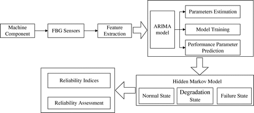
The VRM performance reliability assessment procedure fuses and utilizes the historical sensing monitoring data with the objective of obtaining the performance degradation model and assessing degradation conditions of the equipment and further predicting its reliability changing trend. The proposed equipment performance reliability assessment method is presented in Figure 1. The condition monitoring data is collected in real-time by the Fiber Bragg grating (FBG) sensors and is processed by the signal processing algorithm. Then, a performance degradation path based on ARIMA model is developed to fit the trend of the monitoring vibration data and predict the future data values. The discrete HMM for multi-observation is trained with redefined forward-backward algorithm to recognize the health states and analyze the performance reliability. The effectiveness of the proposed performance reliability assessment system is validated on a VRM test-bed.

Figure 1. System framework for machine reliability analysis.

3.1. Equipment performance parameters monitoring of VRM

As most faults of VRM relate to hydraulic pressure of loading system and mechanical vibration, it’s necessary to conduct hydraulic monitoring and vibration monitoring. These monitoring data describe running state of VRM and provide the essential data base for performance reliability assessment.

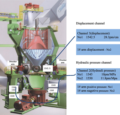
With analysis of the structure and working principle of VRM’s hydraulic loading system, the condition of hydraulic cylinder changes with the hardness of feeding materials. Working performance of VRM is closely related to the running state of the hydraulic loading system, and the latter directly affects throughout, fine powder ratio, particle shape and life of parts of VRM. Hence in this paper, through deploying the hydraulic monitoring points in the hydraulic loading system, monitoring the change of hydraulic in the system and establishing the dynamic properties of the system, which supplies the data base of performance reliability assessment of VRM. The distribution of hydraulic monitoring points of VRM is shown in Figure 2.

Figure 2. Displacement and hydraulic monitoring points of VRM.

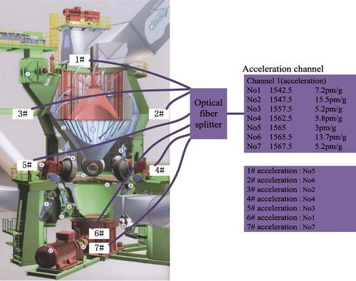
In addition, most faults of VRM relate to mechanical vibration. In order to obtain the current state of VRM and provide data base of performance reliability assessment, it’s necessary to conduct vibration monitoring for VRM. Vibration of the shell caused by change of material layer and hydraulic system can be obtained through vibration monitoring of VRM. Based on the structure modelling and random vibration analysis of the key subsystem of VRM, such as hydraulic loading system, millstone, grinding roller, the natural frequencies and modes of VRM’s shell can be obtained, so as corresponding results of stress, displacement, acceleration. Furthermore, based on theoretical analysis and engineering data validation, important positions of the shell where the change of running state parameters including stress, displacement and acceleration are sharp, where corresponding FBG-based sensors are installed to conduct validation monitoring. The distribution of displacement and acceleration monitoring points of VRM is shown in Figure 2 and 3 respectively. As the carrier of system running state information, dynamic characteristics of mechanical vibration signal contain various equipment abnormalities and fault information. Hence the appropriate arrangement of vibration monitoring points is significant importance for highly efficient vibration monitoring system.

Figure 3. Acceleration monitoring points of VRM’s shell.

There are several vibration excitations form the subsystems of the running VRM, including powder selecting machine, feeding subsystem and hydraulic subsystem, which effect on the vibration and shifting of the shell. As the key component to connect the upper and lower shell of VRM, the bolt will be affected by the tightening force with the shells vibration. Furthermore, the shifting between the upper and lower shell will cause the corresponding changes in the stress of the bolt. Therefore, the stress of the bolt is considered as an important parameter for vibration monitoring of VRM. In the powder selecting machine of VRM, the vibration effect on the connection bolt between shells cause the uneven distribution of tightness, which will result in material running of the connecting part between shells, airflow disorganization and pressure differential in the grinding chamber. The stress and acceleration sensors need be deployed in these locations of the powder selecting subsystem. For the millstone and milling roller components, the fiber Bragg grating displacement sensors are deployed to monitoring the displacement signal in real time, which indirectly reflects the interaction between the millstone and milling roller. In addition, combination with the above physical signals, the running condition of VRM equipment can be monitored with these important parameters. These multiple sensing signals are acquired with various corresponding FBG-based sensors at important monitoring points of VRM, and then feature information of these signals is provided as the input of following reliability assessment model of VRM.

3.2. Performance degradation path based on ARIMA model

The ARIMA model is a widely using time series analysis model for non-stationary random signals. An ARIMA process consists of three components: auto-regressive (AR), differencing and moving average, which is the extension of the well-defined ARMA model by adding the differencing process to transform non-stationary time series into stationary.

In ARIMA model, the future value of a variable is supposed to be the linear combination of several past observations and random errors, and the dynamic system equation can be expressed as follows:(1) $$(1-\sum _{k=1}^p{\mathit{\theta }}_{kj}{B}^k){(1-B)}^d{y}_{ij}=(1-\sum _{k=1}^q{\mathit{\phi }}_{kj}{B}^k){\mathit{\epsilon }}_{ij}$$(1)

where y_ij ε {(T, Y)|(t_i, y_ij); i = 1, 2, …, n; j = 1, 2, …, m} is an observing time series, and the left part is the auto-regressive model with the order p, in which the current series value y_ij is the function of several p-step-before values with the coefficients ${\mathit{\theta }}_{kj}(k=1,\cdots ,p)$, and having the form as:(2) $$x_{ij}=\sum _{k=1}^p{\mathit{\theta }}_{kj}{x}_{(i-k)j}+Z_{ij}$$(2)

where x_ij is stationary time series after the process x_ij = ∇^dy_ij，and Z_ij is the measurement error. The right part of Equation (1) is termed as moving average model with order q, and the ε_ij represents the random error or independent white noise with the coefficients ${\mathit{\phi }}_{kj}(k=1,\cdots ,q)$.(3) $$Z_{ij}={\mathit{\epsilon }}_{ij}-\sum _{k=1}^q{\mathit{\phi }}_{kj}{\mathit{\epsilon }}_{(i-k)j}$$(3)

B is the back-shift operator with the definition as:(4) $$B^k{y}_{ij}=y_{(i-k)j}$$(4)

d is the degree of differencing, and the relationship between the difference operator and the delay operator is given as below:(5) $$\mathrm{\nabla }=1-B$$(5)

The parameters estimation of the ARIMA (p, d, q) model is important. The p, q can be determined using the Akaike information criterion (AIC) by minimizing the information function $f(p,q)=nln{\mathit{\sigma }}_{\mathit{\epsilon }}^2+2(p+q+1)$, which can be done with the optimization procedure.

3.3. Hidden Markov model

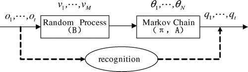
HMM is the evolution of general Markov chain, which contains double stochastic process: a Markov chain with implicit state, and a random observation process. In a standard HMM, a state generates a single observation where the implicit states can be sensed by the visible observation. Suppose that the number of hidden states is N and $q_t\in ({\mathit{\theta }}_1),\dots ,{\mathit{\theta }}_N$ is the state at time point t, and let $o_t\in (v_1,\dots ,v_M)$be the observation at time t where M is the number of observations. The mapping of hidden states and observations is illustrated in Figure 4.

Figure 4. Mapping of hidden state and observation for HMM.

A HMM is characterized by its parameters: the initial state distribution π = (π₁, …, π_N), the state transition probability $A={(a_{ij})}_{N\times N}$ and the conditional probability distribution of observation $B={(b_{jk})}_{N\times M}$. ${\mathit{\pi }}_{\text{i}}=P(q_1={\mathit{\theta }}_i)$ is the probability that the initial state is θ_i, and $a_{ij}=P(q_{t+1}={\mathit{\theta }}_j|q_t={\mathit{\theta }}_i)$ is the transition probability from state θ_i to state θ_j, and $b_{jk}=P({\text{o}}_t={\mathit{\nu }}_k|q_t={\mathit{\theta }}_j)$ is the observed probability of v_k with the state θ_j. In general, the HMM can be described as $\mathit{\lambda }=(A,B,\mathit{\pi })$.

In real applications, there are three important algorithms associated with HMM:

(1) Forward-backward algorithm: Given the observation sequence $O=\{o_1,\dots ,o_T\}$ and the HMM $\mathit{\lambda }=(A,B,\mathit{\pi })$, we use the forward-backward algorithm to compute the probability of the observation sequence.

The forward variable ${\mathit{\alpha }}_t(i)$ is defined as ${\mathit{\alpha }}_t(i)=P({\text{o}}_1,\dots ,o_t,q_t={\mathit{\theta }}_i|\mathit{\lambda })$, which means the probability of the observed sequence $\text{{}{o}_1,\dots ,o_t\text{}}$ at time point t and end in state θ_i. The ${\mathit{\alpha }}_t(i)$ can be initialized as follow:(6) $${\mathit{\alpha }}_t(i)={\mathit{\pi }}_i{b}_{i1}$$(6)

Then, the recursive equation can be written as:(7) $${\mathit{\alpha }}_{t+1}(j)=[\sum _{i=1}^N{\mathit{\alpha }}_t(i)a_{ij}]b_{j(t+1)},1|\le t\le T-1,1\le j\le N$$(7)

where $b_{j(t+1)}=P(O_{t+1}={\mathit{\nu }}_k|q_t={\mathit{\theta }}_j)$.

The probability of the observation sequence $O=o_1,\dots ,o_T\}$ given in the model $\mathit{\lambda }(A,B\mathit{\pi })$ can be obtained:(8) $$P(O|\mathit{\lambda })=\sum _{i=1}^N{\mathit{\alpha }}_T(i)$$(8)

With the opposite recursive direction, the backward variable is defined as follows:(9) $${\mathit{\beta }}_t(i)=\sum _{j=1}^N{\mathit{\beta }}_{t+1}(j)a_{ij}{b}_{j(t+1)}$$(9)

(2) Viterbi algorithm: Given the observation sequences $O=\{o_1,\dots ,o_T\}$ and the HMM $\mathit{\lambda }=(A,B,\mathit{\pi })$, we use the Viterbi algorithm to estimate the relative optimal state sequences. The forward variable can be defined as the maximum probability of observation sequences $O=\{o_1,\dots ,o_T\}$ with the state sequences $\{q_1,\dots ,q_{t-1}\}$ and end in state θ_i:(10) $${\mathit{\gamma }}_t(i)=\underset{1\le i\le N}{Max}P(q_1,\dots ,q_{t-1},q_t={\mathit{\theta }}_i,o_1,\dots ,o_t|\mathit{\lambda })$$(10)

(3) Baum-Welch algorithm: Given the observation sequences $O=\{O_1,\cdots ,o_T\}$, we use the Baum-Welch algorithm to calculate the parameters of HMM $\mathit{\lambda }=(A,B,\mathit{\pi })$ to maximize $P(O|\mathit{\lambda })$.

3.3. Multi-observation-based HMM for reliability assessment

3.3.1. Inference for multi-observation HMM

The general HMM is applied in single observation sequence, while the VRM is monitored by a group of sensors. Thus, it needs to propose a modified training algorithm to reestimate all parameters of the HMM under the multi-observation sequences.

Assume that the multi-observation sequences set is $O=\{O^{(1)},\dots ,O^{(L)}\}$, and the $O^{(l)}=\{o_1^{(l)},\dots ,o_T^{(l)}\}$ is defined as the observation sequence of a single sensor which is independent of other observed sequences. In the multi-observation HMM, the observed probability distribution is determined by multiple observation sequences, as opposed to a single observation sequence in the general HMM. In this paper, the observed probability $b_j(O_t)$ for multi-observation sequences $O_t=\{O_t^{(1)},\dots ,O_t^{(L)}\}$ is written as follow:(11) $$\begin{array}{cc}{b}_j(o_t^{(1)}\dots o_1^{(L)})\hfill & =P(o_t^{(1)}\dots o_t^{(L)}|q_t={\mathit{\theta }}_j)\hfill \\ \hfill & =P(o_t^{(1)}|q_t={\mathit{\theta }}_j)\dots P(o_t^{(L)}|q_t={\mathit{\theta }}_j)\hfill \\ \hfill & =b_j(o_t^{(1)})\dots b_j{o}_t^{(L)}\hfill \end{array}$$(11)

The forward variable for multi-observation sequences is denoted as:(12) $${\mathit{\alpha }}_t(i)=P(o_1^{(1)}\dots o_1^{(L)},\dots ,o_t^{(1)}\dots o_t^{(L)},q_t={\mathit{\theta }}_i|\mathit{\lambda })$$(12)

With the independence of the multiple observation sequences, the forward variable can be simplified as a follow:(13) $$\begin{array}{cc}{\mathit{\alpha }}_t(i)\hfill & =P(o_1^{(1)}\dots o_t^{(1)},\dots ,o_t^{(L)}\dots o_t^{(L)},q_t={\mathit{\theta }}_i|\mathit{\lambda })\hfill \\ \hfill & =P(o_1^{(1)}\dots o_t^{(1)},q_t={\mathit{\theta }}_i|\mathit{\lambda })P(o_1^{(2)}\dots o_t^{(2)},\dots ,o_t^{(L)}\dots o_t^{(L)},q_t={\mathit{\theta }}_i|\mathit{\lambda })\hfill \\ \hfill & =P(o_1^{(1)}\dots o_t^{(1)},q_t={\mathit{\theta }}_i|\mathit{\lambda })P(o_1^{(2)}\dots o_t^{(2)},q_t={\mathit{\theta }}_i|\mathit{\lambda })\dots P(o_1^{(L)}\dots o_t^{(L)},q_t={\mathit{\theta }}_i|\mathit{\lambda })\hfill \\ \hfill & ={\mathit{\alpha }}_t^{(1)}(i){\mathit{\alpha }}_t^{(2)}(i)\dots {\mathit{\alpha }}_t^{(L)}(i)\hfill \end{array}$$(13)

where ${\mathit{\alpha }}_t^{(l)}(i)=P(o_1^{(l)}\cdots o_1^{(l)},q_t={\mathit{\theta }}_i|\mathit{\lambda })$.

Then, the forward recursion formula is obtained as:(14) $${\mathit{\alpha }}_{t+1}(j)=\left(\sum _{i=1}^N{\mathit{\alpha }}_t(i)a_{ij}\right)·b_j(o_{t+1}^{(1)},\dots ,o_{t+1}^{(L)})$$(14)

Given state θ_i, the initial condition is defined at time t = 1:(15) $${\mathit{\alpha }}_1(i)={\mathit{\pi }}_i\dots b_i(o_1^{(1)},\dots ,o_1^{(L)})$$(15)

The backward variable, for multi-observation sequences is shown as below:(16) $$\begin{array}{cc}{\mathit{\beta }}_t(i)\hfill & =P(o_{t+1}^{(1)}\dots o_{t+1}^{(L)},\dots ,o_T^{(1)}\dots o_T^{(L)}|q_t={\mathit{\theta }}_i,\mathit{\lambda })\hfill \\ \hfill & ={\mathit{\beta }}_t^{(1)}(i){\mathit{\beta }}_t^{(2)}(i)\dots {\mathit{\beta }}_t^{(L)}(i)\hfill \end{array}$$(16)

And the following backward recursion formula:(17) $${\mathit{\beta }}_t(i)=\sum _{j=1}^N{a}_{ij}{b}_j(o_{t+1}^{(1)},\dots ,o_{t+1}^{(L)}){\mathit{\beta }}_{t+1}(j)$$(17)

The initial condition at time t = T:(18) $${\mathit{\beta }}_T(i)=1$$(18)

Based on the above inference, the parameters of HMM can be reestimated under the multi-observation sequences. Firstly, the variable ${\mathit{\xi }}_t(i,j)$ is defined to express the transition probability from state θ_i to state θ_j at time t under observation sequence $O_1^T$ and model $\mathit{\lambda }$.(19) $$\begin{array}{cc}{\mathit{\xi }}_t(i,j)=P(q_t\hfill & ={\mathit{\theta }}_i,q_{t+1}={\mathit{\theta }}_j|O_1^T,\mathit{\lambda })\hfill \\ \hfill & =\left({\mathit{\alpha }}_t(i)a_{ij}{b}_j(o_{t+1}^{(1)},\dots ,o_{t+1}^{(L)}){\mathit{\beta }}_{t+1}(j)\right)/P(O_1^T|\mathit{\lambda })\hfill \end{array}$$(19)

And the probability of stay in state θ_i at time t, given the observation sequence $O_1^T$ and $\mathit{\lambda }$ is defined as ${\mathit{\gamma }}_t(i)$.(20) $$\begin{array}{cc}{\mathit{\gamma }}_t(i)\hfill & =P(q_t={\mathit{\theta }}_i|O_1^T,\mathit{\lambda })\hfill \\ \hfill & =\left({\mathit{\alpha }}_t(i){\mathit{\beta }}_t(i)\right)/P(O_1^T|\mathit{\lambda })\hfill \end{array}$$(20)

In the Equations (19) and (20) the probability of multi-observation sequences given the HMM $\mathit{\lambda }$ (i.e. $P(O_1^T|\mathit{\lambda })$) can be written as the weighted summation of all the probability of the single observation sequence:(21) $$P(O_1^T|\mathit{\lambda })=\sum _{l=1}^L{w}_{l}P(O_1^{(l)}T|\mathit{\lambda })$$(21)

where $w_l=\frac{1}{L}P(O^{(l+1)}|O^{(l)},\mathit{\lambda })\dots P(O^{(l-1)}|O^{(l)}{O}^{(l-2)}\dots O^{(1)},\mathit{\lambda })$.

Then, the parameters reestimation formulae of the HMM can be derived under the multi-observation sequences.

The initial state distribution is the probability that the first state is θ_i :(22) $$\overline{{\mathit{\pi }}_i}={\mathit{\gamma }}_t(i)$$(22)

The reestimation formula of state transition probabilities a_ij is the ratio of the number of transitions from state θ_i to state θ_j, to all the number of transitions from state θ_i.(23) $$\overline{a_{ij}}=\frac{{\sum }_{t=1}^{T-1}{\mathit{\xi }}_t(i,j)}{{\sum }_{t=1}^{T-1}{\mathit{\gamma }}_t(i)}$$(23)

The reestimation formula of observation probabilities b_jk is the ratio of the number of observation value v_k at state θ_j, to all the number of state θ_j.(24) $$\overline{b_{jk}}=\frac{{\sum }_{t=1,o_t={\mathit{\nu }}_k}^T{\mathit{\gamma }}_t(j)}{{\sum }_{t=1}^T{\mathit{\gamma }}_t(j)}$$(24)

3.4.2. Reliability assessment of VRM

The initial discrete HMM of VRM based on the condition monitoring information is established, where the initial state probability distribution π₀ = (1, 0, …, 0) and A₀, B₀ is obtained with the uniform or non-zero random distribution. Based on the initial HMM and multi-observation sequences, the convergence model $\mathit{\lambda }=(A,B,\mathit{\pi })$ is trained by using modified forward-backward algorithm, and the rationality of the model is verified.

The performance reliability of VRM at any time point can be assessed using the valid multi-observation HMM. Assume that the probability of stay in state θ_j at time t is P_j(t) = P(q_t = j), and according to the Chapman Kolmogorov equation, the probability differential equation can be written as:(25) $$P^{\prime }(t)=P(t)·A$$(25)

where P(t) = (P₀(t), P₁(t), …, P_k(t), P_(k+1)(t)) is the state probability distribution vector at time point t, and $P^{\prime }(t)$ is the first order differential result of P(t), and A is the system state transition probability matrix.

The representation of P(t)can be obtained by solving the differential equation in Equation (25), and is expressed as:(26) $$P(t)=e^{At+C}$$(26)

where C is a constant vector, $C={[C_1,\dots ,C_k,C_{k+1}]}^T$.

Suppose that the equipment is in normal condition at the initial time, thus:(27) $$P(0)=(P_0(0),P_1(0),\dots ,P_k(0),P_{(k+1)}(0))=(1,0,\dots ,0,0)$$(27)

Substituting state transition matrix $\text{A}$and initial probability P(0) into Equation (26), $C={[C_1,\dots ,C_k,C_{k+1}]}^T$ can be calculated, and state probability distribution vector at time point t $P(t)=(P_0(t),P_1(t),\dots ,P_k(t),P_{(k+1)}(t))$ can be obtained after substitute C into it. Then, the reliability assessment formula $R(t)=1-P_{(k+1)}(t)$ is used to obtain the performance indexes of VRM.

4. Experiment and model development

4.1. Data acquisition

The proposed method is applied to assess the performance reliability of a VRM equipment. In order to monitor the equipment running condition, several physical signals were collected such as temperature, displacement, speed, acceleration, torque, and dynamic strain. These signals were acquired through FBG sensors on the vertical mill. Among all the signals, the strain and displacement signals are always used to present the change of hydraulic loading pressure, the displacement and velocity of the piston in the hydraulic system when the load of VRM changes.

The dynamic characteristics of the above two sensing monitoring data were fused to judge the torsional vibration of mill drive system. In this experiment, the performance degradation path of VRM equipment is built with the ARIMA model using the hydraulic pressure and displacement signal. Then, the multi-observation HMM is used to create a mapping between the sensor data and real performance reliability of the equipment.

4.2. Experiment results and discussion

4.2.1. Performance degradation model based on ARIMA

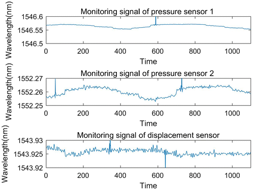
The experimental data is acquired at the frequency of 4 KHz, and processed using wavelet packet with Symlets wavelet 5 (sys10) to reduce the noise. The data sampling is conducted to obtain the test data from the mass long-term monitoring raw data, and then a mean value processing for every 0.5s is applied. After this, the 1,100 sets of hydraulic and displacement signal with the time span of 550s are obtained, which are shown in Figure 5. For each of the data sample, the first 1,000 points are selected as the model training data, and the last 100 points are used as test data.

Figure 5. The characteristic value sampling of the operating parameters.

The ARIMA, as a time series analysis method, is applied to model the performance degradation of sensitive parameters based on the historical sensing monitoring data, and establish a performance degradation path to predict the future values. The ARIMA based performance degradation model generally includes three parts: model identification, parameter estimation, and effectiveness verification checking. Taking the positive pressure operating signal of the pressure sensor 1 as an example, firstly, the stationary characteristic of the pressure signal is analyzed, and difference process is carried out with the non-stationary analysis result. Then, the autocorrelation function and partial autocorrelation function are calculated, and the AIC criterion is applied to identify the model and determine the order of AR and MA. The calculation result shows that the information function of the model reached a minimum value when is (2, 4). Based on the result of differential operation, the ARIMA model is determined as ARIMA (2, 1, 4). Next, the model parameters of ARIMA (2, 1, 4) are determined through nonlinear least squares method, and the results are shown in Table 1.

Table 1. Parameter estimation of ARIMA model for the positive pressure signal

Variables	Coefficients	Variables	Coefficients
AR (1)	−1.998	MA (1)	−1.933
AR (2)	0.9985	MA (2)	0.9256
–	–	MA (3)	0.002142
–	–	MA (4)	0.004805

Finally, the prediction performance of the ARIMA model is verified with the last 100 testing data, and the relative prediction error is 5.3898 e-003, which can illustrate the validity of the model.

Similar to the positive pressure of the hydraulic pressure sensor, the performance deterioration model of the native pressure and the displacement parameters of VRM are established respectively.

The negative pressure deterioration model is determined as ARIMA (1, 1, 3), and the parameters are shown in Table 2.

Table 2. Parameter estimation of ARIMA model for the negative pressure signal

Variables	Coefficients	Variables	Coefficients
AR (1)	−0.9965	MA (1)	−0.7157
–	–	MA (2)	−0.03432
–	–	MA (3)	−0.07581

The displacement deterioration model is determined as ARIMA (2, 1, 2), and the parameters are shown in Table 3.

Table 3. Parameter estimation of ARIMA model for the displacement signal

Variables	Coefficients	Variables	Coefficients
AR (1)	−1.14	MA (1)	−0.936
AR (2)	0.149	MA (2)	0.2338

4.2.2. Performance reliability assessment based on multi-observation HMM

The proposed performance degradation model based on the ARIMA method of VRM can be used to predict a series of performance degradation data of VRM at a certain moment or a period of time in the future. Based on these data, the discrete multi-observation HMM is used to evaluate the reliability changing trend of VRM.

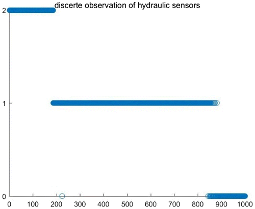
In order to get the discrete observation sequences, the continuous time series need to be quantized. In this paper, the Lloyd algorithm is used to quantize the continuous multi-sensing monitoring signals and fuse multiple feature signals. The system partition vector and codebook vector of the multi-sensing monitoring signals are established using the experience knowledge.

According to the working requirements of VRM, the health states of the equipment are divided into three categories: normal, slight deterioration and serious deterioration. Taking the hydraulic pressure signal as an example, the partition criterion of pressure signal is showed in Table 4.

Table 4. The failure criterion of hydraulic pressure sensor

Hydraulic range (Mpa)	Wavelength variation (pm)	Deterioration degree
(4, 13)	(40, 130)	Normal
(3, 4) or (13, 14)	(30, 40) or (130, 140)	Slight deterioration
(0, 3) or (14, ∞)	(0, 30) or (140, ∞)	Serious deterioration

Based on the Lloyd algorithm, the output discrete observation sequences of hydraulic pressure signal and displacement signal data are obtained, and the discrete observation sequences of hydraulic pressure signal is shown as Figure 6.

Figure 6. The discrete observation sequences of hydraulic pressure signal.

In this paper, a HMM with three states is utilized to estimate the reliability changing trend of VRM equipment. Firstly, the initial parameters of HMM are assumed: the initial state probability distribution π₀ = [1, 0, 0]^T; the state transition probability A₀ and observation probability matrix B₀ are selected with the random method.$$A_0=\left[\begin{array}{ccc}0.5117\hfill & 0.0295\hfill & 0.4588\hfill \\ 0\hfill & 0.0717\hfill & 0.9283\hfill \\ 0\hfill & 0\hfill & 1.0000\hfill \end{array}\right]B_0=\left[\begin{array}{ccc}0.0772\hfill & 0.7624\hfill & 0.1604\hfill \\ 0.3767\hfill & 0.3579\hfill & 0.2654\hfill \\ 0.3639\hfill & 0.1130\hfill & 0.5231\hfill \end{array}\right]$$

Based on the initial model ${\mathit{\lambda }}_0=(A_0,B_0,{\mathit{\pi }}_0)$ and the multi-observation sequences of VRM, the parameters of the multi-observation HMM are estimated with the parameter reestimation algorithm mentioned in Section 3.4.1. The model parameters $\overline{{\mathit{\pi }}_i}$, $\overline{a_{ij}}$ and $\overline{b_{ij}}$ are presented as follows:$$\mathit{\pi }=\left[\begin{array}{c}1\hfill \\ 0\hfill \\ 0\hfill \end{array}\right]A=\left[\begin{array}{ccc}0.9523\hfill & 0.0477\hfill & 0\hfill \\ 0\hfill & 0.9990\hfill & 0.0010\hfill \\ 0\hfill & 0\hfill & 1\hfill \end{array}\right]B=\left[\begin{array}{ccc}0.9767\hfill & 0.0233\hfill & 0\hfill \\ 0.0069\hfill & 0.9928\hfill & 0.0003\hfill \\ 0\hfill & 1\hfill & 0\hfill \end{array}\right]$$

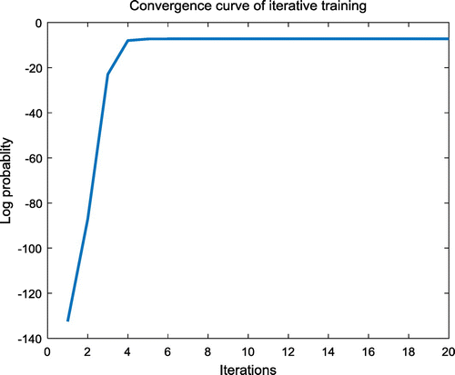
The convergence curve of iterative training process shows in Figure 7, which shows that the log-likelihood increases with the iterations, and the log-likelihood is convergent at iteration 7.

Figure 7. Convergence curve of iterative training.

Based on the model $\mathit{\lambda }=(A,B,\mathit{\pi })$, the performance reliability of VRM at a certain time point are calculated with the Equation (26), the state vector $P(t)=(P_0(t),P_1(t),P_2(t))$ of the VRM equipment at time t is obtained, hence the change trend of reliability expressed as R(t) = 1 − P₂(t) is obtained, as shown in Figure 8.

Figure 8. Reliability changing curve.

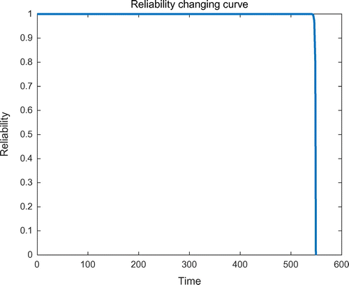
From Figure 8, it shows that VRM is in the deterioration when the reliability is lower than 0.8, the probability of a failure is extremely large. Hence the reliability can be used as the index to describe the state of VRM in practical applications clearly and accurately.

5. Conclusions

This paper researches the performance degradation problem of VRM, and proposes a performance reliability assessment method based on ARIMA and multi-observation HMM for VRM reliability assessment. Most fault information of VRM store in hydraulic pressure of loading system and vibration signals, thus, hydraulic monitoring and vibration monitoring are introduced to determine the monitoring points and sensing parameters, which is also the data base of reliability assessment. Then the ARIMA method is applied to fit and predict the performance parameters, and further obtain the performance degradation path of the equipment. Finally, a discrete Hidden Markov Model (HMM) based on multi-observation is provided to cater for the multi-sensing monitoring characteristic of VRM, and it is used to evaluate the performance reliability changing characteristic of VRM. At the end of the research, the historical monitoring data is applied to the proposed method to determine validity and practicability. The result shows that the proposed assessment approach is effective for equipment performance reliability assessment and health condition management.

Acknowledgments

The authors are grateful to the case companies for their constructive contribution.

Additional information

Funding

This work was supported by National Natural Science Foundation of China [grant number 51475343], Fundamental Research Funds for the Central Universities [grant number 2015III003], International Science and Technology Cooperation Program of China [2015DFA70340].

Notes on contributors

Qiang Wang

Qiang Wang is a doctor of the school of information engineering at the Wuhan University of Technology. His research interests are in the field of Fiber Bragg Grating sensing, signals processing, mechanical condition monitoring and intelligent perception.

Yilin Fang

Yilin Fang is an associate professor of the school of information engineering at the Wuhan University of Technology. His doctoral degree was obtained from Wuhan University of Technology in 2010. His research interests are in the field of machine learning, machinery fault diagnosis and network protocol architecture and algorithms.

References

- Alshraideh, H., & Runger, G. (2014). Process monitoring using hidden Markov models. Quality and Reliability Engineering International, 30, 1379–1387.10.1002/qre.v30.8
- Amin, A., Grunske, L., & Colman, A. (2013). An approach to software reliability prediction based on time series modeling. Journal of Systems and Software, 86, 1923–1932.10.1016/j.jss.2013.03.045
- Boutros, T., & Liang, M. (2011). Detection and diagnosis of bearing and cutting tool faults using hidden Markov models. Mechanical Systems and Signal Processing, 25, 2102–2124.10.1016/j.ymssp.2011.01.013
- Caesarendra, W., Widodo, A., Thom, P. H., Yang, B. S., & Setiawan, J. D. (2011). Combined probability approach and indirect data-driven method for bearing degradation prognostics. IEEE Transactions on Reliability, 60, 14–20.10.1109/TR.2011.2104716
- Caesarendra, W., Widodo, A., & Yang, B. S. (2010). Application of relevance vector machine and logistic regression for machine degradation assessment. Mechanical Systems and Signal Processing, 24, 1161–1171.10.1016/j.ymssp.2009.10.011
- Chen, D. (2012). Reliability analysis of multi-state system based on fuzzy bayesian networks and application in hydraulic system. Journal of Mechanical Engineering, 48, 175–183.10.3901/JME.2012.16.175
- Comert, G., & Bezuglov, A. (2013). An online change-point-based model for traffic parameter prediction. IEEE Transactions on Intelligent Transportation Systems, 14, 1360–1369.10.1109/TITS.2013.2260540
- Di Maio, F., Tsui, K. L., & Zio, E. (2012). Combining relevance vector machines and exponential regression for bearing residual life estimation. Mechanical Systems and Signal Processing, 31, 405–427.10.1016/j.ymssp.2012.03.011
- Gao, C., Jiang, M., Huang, J. Y., & Wang, X. F. (2012). Degradation path modeling method based on time series analysis. In Applied mechanics and Materials (Vol. 121, pp. 2205–2210). Zurich: Trans Tech Publications.
- Geramifard, O., Xu, J. X., Zhou, J. H., & Li, X. (2012). A physically segmented hidden Markov model approach for continuous tool condition monitoring: Diagnostics and prognostics. IEEE Transactions on Industrial Informatics, 8, 964–973.10.1109/TII.2012.2205583
- Harrell, F. (2015). Regression modeling strategies: with applications to linear models, logistic and ordinal regression, and survival analysis. Cham: Springer.10.1007/978-3-319-19425-7
- Jiang, H., Chen, J., & Dong, G. (2016). Hidden Markov model and nuisance attribute projection based bearing performance degradation assessment. Mechanical Systems and Signal Processing, 72–73, 184–205.10.1016/j.ymssp.2015.10.003
- Jiang, L., Liu, Y., Li, X., & Chen, A. (2011). Degradation assessment and fault diagnosis for roller bearing based on ar model and fuzzy cluster analysis. Shock and Vibration, 18, 127–137.10.1155/2011/703210
- Lee, J., Wu, F., Zhao, W., Ghaffari, M., Liao, L., & Siegel, D. (2014). Prognostics and health management design for rotary machinery systems—Reviews, methodology and applications. Mechanical Systems and Signal Processing, 42, 314–334.10.1016/j.ymssp.2013.06.004
- Liu, T., Chen, J., & Dong, G. (2013). Zero crossing and coupled hidden Markov model for a rolling bearing performance degradation assessment. Journal of Vibration and Control. doi:10.1177/1077546313479992
- Loutas, T. H., Roulias, D., & Georgoulas, G. (2013). Remaining useful life estimation in rolling bearings utilizing data-driven probabilistic e-support vectors regression. IEEE Transactions on Reliability, 62, 821–832.10.1109/TR.2013.2285318
- Pani, A. K., & Mohanta, H. K. (2015). Online monitoring and control of particle size in the grinding process using least square support vector regression and resilient back propagation neural network. ISA Transactions, 56, 206–221.10.1016/j.isatra.2014.11.011
- Visser, I. (2011). Seven things to remember about hidden Markov models: A tutorial on Markovian models for time series. Journal of Mathematical Psychology, 55, 403–415.10.1016/j.jmp.2011.08.002
- Wang, P., & Coit, D. W. (2007, January). Reliability and degradation modeling with random or uncertain failure threshold. In 2007 Annual Reliability and Maintainability Symposium (pp. 392–397). Washington, DC: IEEE.10.1109/RAMS.2007.328107
- Wei, R. P., & Harlow, D. G. (2004). Mechanistically based probability modelling, life prediction and reliability assessment. Modelling and Simulation in Materials Science and Engineering, 13, 33–51.
- Xia, L., Fang, H., & Zhang, H. (2013, May). HMM based modeling and health condition assessment for degradation process. In 2013 25th Chinese Control and Decision Conference (CCDC) (pp. 2945–2948). Washington, DC: IEEE.10.1109/CCDC.2013.6561449
- Xiao, W. B., Chen, J., Dong, G. M., Zhou, Y., & Wang, Z. Y. (2012). A multichannel fusion approach based on coupled hidden Markov models for rolling element bearing fault diagnosis. Proceedings of the Institution of Mechanical Engineers, Part C: Journal of Mechanical Engineering Science, 226, 202–216.
- Zhang, L., Feng, F., & Bi, M. (2015, October). Reliability assessement method based on SVDD and SVR with multiple performances degradation data for chassis system. In Reliability Systems Engineering (ICRSE), 2015 First International Conference (pp. 1–5). Washington, DC,: IEEE.
- Zheng-jia, H., Hong-rui, C., & Yan-yang, Z. (2014). Developments and thoughts on operational reliability assessment of mechanical equipment [J]. Journal of Mechanical Engineering, 50, 171–186.