A note on estimating minimal changeover time

Abstract

We propose a novel approach for the estimation of change-over times in a continuous production environment, and discuss the importance and prospects of our suggested framework through an illustrative example.

Keywords:

• setup time
• changeover time
• shortest path
• SMED

Public Interest Statement

We present a novel approach for estimation of setup times when changing system configuration. We adapt a robotic movement algorithm to do this. We are able to show that our suggested approach outperforms an acceptable benchmark approach in a statistically significant manner.

1. Introduction

Setup times and their crucial role in the efficiency and costs associated with production and manufacturing systems have been extensively studied (e.g. Allahverdi, Gupta, & Aldowaisan, 1999; Allahverdi, Ng, Cheng, & Kovalyov, 2008; Leon & Peters, 1996; Smed, Salonen, Johnsson, Johtela, & Nevalainen, 2003, among others). The importance of shortening these setup times is discussed in a recent editorial by Allahverdi and Soroush (2008), and has been a focal point in applications of Shingo’s “Single Minute Exchange of Die” (SMED) method Shingo (1985), e.g. Cakmakci and Karasu (2006), Shinde, Jahagirdar, Sane, and Karandikar (2014), and Stadnicka (2015) to name a few. However, to the best of our knowledge, in many settings these setup times are given as model parameters (c.f. Baker and Trietsch (2013) and references therein).

In this note we set-forth a new approach with respect to setup times, and present a novel procedure for estimation of a minimal changeover time. Our approach is an adaptation of recent advances in the field of real-time motion planning when avoiding obstacles (Shvalb, Moshe, & Medina, 2013). While applications of our idea are abundant in process manufacturing settings, we were motivated through our cooperation with a leading manufacturer from the non-woven cloths industry, where production is a continuous process (ongoing 24/7), and a variety of different products (i.e. with a set of different desired properties—see for example http://www.avgol.com/technology-product/general.aspx) may be manufactured in the same facility and using the same process. The importance of minimizing changeover (or setup) times is both in the maximization of capacity (better utilization of time), and in minimizing production of waste. Both of these aspects, and the importance of the SMED method, are discussed in a recent comprehensive review of the relevant literature by Panwar, Nepal, Jain, and Rathore (2015).

The production process that our industry partner carries out is one where melted polypropylene filaments are injected onto a moving conveyor belt, creating a sheet of fiber, which is then pressed and treated to give it a desired set of properties, rolled, and eventually cut to desired size. The difference between products is achieved using a combination of certain production parameters (e.g. the temperature, diameter of the thread being injected, pressure, speed, etc.). We refer to a specific set of production parameters as a configuration. There is a unique mapping between a configuration and a product. Further, a change between products is a change between configurations, and the product produced during the changeover period is waste—i.e. there is a clear benefit from minimizing the changeover time. It turns out that changing between configurations is a challenging and possibly delicate issue. Specifically, if certain configurations occur while changeover takes place, there is a greater probability, and in some settings even certainty, that the resulting final configuration (i.e. product) will be defective. In our example this means that there would be a rips in the threads that makeup the fabric, and in-turn, the final fabric will not achieve the desired properties.

While there is a large variety of products, it turns out that due to years of trial and error, there is vast knowledge of which configurations should be avoided (i.e. it is possible to construct functions describing which configurations should be avoided). Further, when changeover occurs, the production technicians control the changeover by manipulating production parameters one-by-one, avoiding certain “areas” of configurations, in order to minimize probability of producing defects.

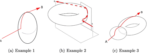
As system configuration change is required to achieve the change between products, and since the longer it takes to changeover the more waste is created, we need to find a feasible shortest path between these combinations. This change needs to account for the fact that there are parameter combinations that we need to avoid, as these result in product defects. Further, there are parameter combination that are infeasible due to physical constraints on the system (e.g. certain combinations of temperature and pressure, certain combinations of thread diameter and velocity, etc.). These constraints are formulated and we are able to identify a short path satisfying them, while minimizing the time that garbage is produced (i.e. reaching the required production configuration). To illustrate our intention see Figure 1.

Figure 1. Illustrative examples of feasible shortest paths that allow change from Configuration A to Configuration B, avoiding a certain set of configurations.

Currently, changeover between products (or configurations) in our example setting is done in a manual fashion, where operators change configurations by changing parameters in a step-wise manner (i.e. moving between different parameter values until the desired final value is reached), while avoiding parameter combinations that are, based on prior knowledge gained through experience, associated with product defect. Our understanding is, that while there is a potential of automating this process, there would still be a need for some control ensuring avoidance of system configurations that are undesirable (either due to a feasibility constraint, or to avoid product defects). We limit our focus to systems where the configurations are vectors of continuous parameter values, and a functional form of a specific type can be used for both the objective function and constraints on parameter relationships. In the motivating example, it is easy to think of the objective of minimizing the time the change in configuration as it is directly related to the amount of product we must discard (product produced on the conveyor while the system has yet to reach the desired configuration). The constraints that need to be accounted for are both feasibility constraints—e.g. certain temperatures are not sufficient for certain thread diameters, and certain pressure can not accommodate certain speed requirements (for the conveyor belt). We are able to formulate these constraints as functions of the parameters. Finally, as there are certain combinations of parameters that result in defective products we can add these as infeasible combinations. For example, we can put in place a function on parameters representing all configurations that result in at least $95\%$ probability of product defect.

In what follows we outline our mathematical framework, and a Pseudo-algorithm, that provides a detailed path of change between configurations in polynomial time, $O(N^3)$, accounting for constraints. The intuition behind the suggested algorithm is that the shortest path, in case a direct line between the starting configuration and required configuration encounters a constraint (i.e. visiting certain undesirable configurations), is a “crawl” along the constraint until the we can continue the change in a “straight line”. This is illustrated in Figure 3. This approach is an extension of Shvalb et al. (2013) to more than 8-dimensional configuration space, as the original algorithm is limited to, and restricting ourselves to systems with continuous parameters defining the configurations, a reduced effort in calculating how to avoid constraints.

2. Mathematical model—Estimating change over time using a feasible “shortest” path

A configuration c is an ordered list of N independent variables (or parameter values). A configuration space $\mathcal{C}$ is the totality of all such configurations (for a more detailed discussion about configuration spaces see Blanc and Shvalb (2012)). There is a posrtion of $\mathcal{C}$ which is forbidden, we shall denote it by $\mathcal{F}\subset \mathcal{C}$ and suppose $\mathcal{F}$ is comprised of n connected components such that $\mathcal{F}={\dot{\cup }}_{i=1}^n{\mathcal{F}}_i$.

Figure 2. Crawling on the constraints. (A) Crawling on a cylindrical constraint defined by projecting the desired direction v on n’s null-space, k, where $n=\mathrm{\nabla }f$. Motion proceeds in the general direction of $v^{\prime }$. (B) represents a configuration in which maintains two constraints.

We assume that ${\mathcal{F}}_i$ are defined implicitly as the varieties $f_i(x_1,\dots ,x_N)=0$. Recall that a level set a is defined as $f_i(x_1,\dots ,x_N)=a$ which we think of as the distance from all ${\mathcal{F}}_i$. Let $c_s$ and $c_g$ be the initial and the goal configurations respectively and obviously motion between them should be performed within $\mathcal{C}$ avoiding $\mathcal{F}$. Following a similar point of view of CPRM (see Shvalb et al., 2013), we can identify the set of constraints as forbidden sets in $\mathcal{C}$ on which one would like to crawl as the configuration changes (see Figure 2). Given a configuration c, motion on the boundary of $g_i$ (or of a set of constraints $g_i,i\subset I$) is achieved by calculating the normal vector $\widehat{n}=\mathrm{\nabla }g$ (or a set of normals $n_i,i\subset I$) to $g_i$ (respectively) at c. We define a matrix G where each column in it is ${\widehat{n}}_i$. We restrict the motion in $\mathcal{C}$ to its (their) null space ${\mathcal{K}}_I=Null(G)$. We call such a motion scheme “crawling”. We set $\overrightarrow{V}$ to be the normalized motion direction ${\overrightarrow{V}}_d=\frac{c_g-c}{\Vert c_g-c\Vert }$ projected on ${\mathcal{K}}_I$. So, motion proceeds by:(1) $$\begin{array}{c}\hfill c_{k+1}-c_k=\mathit{ϵ}\overrightarrow{V}\end{array}$$(1)

where $\mathit{ϵ}<<1$ is the step size in $\mathcal{C}$. We calculate $\overrightarrow{V}$ by:(2) $$\begin{array}{c}\hfill \overrightarrow{V}=\sum _{i\in I}{\widehat{\mathcal{K}}}_i·{\overrightarrow{V}}_d·{\widehat{\mathcal{K}}}_i^T\end{array}$$(2)

where ${\widehat{\mathcal{K}}}_i$ is the i-th base vector of ${\mathcal{K}}_I$. Hence motion in $\mathcal{C}$ is obtained by repetitively calculating (Equation (1)) until reaching the desired configuration. Algorithm 1 depicts the crawling procedure described.

Using Algorithm 1, and assuming that there is a simple mapping from path length to setup time, we achieve a simple way to estimate a minimal changeover time.

3. Conclusions

To highlight the potential of our approach, we carried out a numeric analysis using simulated data based on our collaboration with an industry partner a non-woven fabric manufacturer. Based on our collaboration we constructed a set of five constraints by randomly selecting coefficients for polynomials of the following form: ${\sum }_{i\in N}{A}_i{X}_i^{a_i}$. For each polynomial $X_i$ are our parameters, N is the dimension of our parameter space, and $A_i$s are drawn from uniform distributions on the range $[-9,9]$, and $a_i$s are drawn from uniform distributions on the range (0, 4]. We carried out hundreds of repetitions for our analysis, and the dimension of our parameter space, for sake of analysis, was from 3 to 10. We compare our results to those achieved by a feasible rectilinear path. A summary of the results, showing the prospects of our approach, are presented in Figure 3. It highlights the not-very-surprising conclusion that choice of how to change configurations effects the change-over time. Further, we note that on average the distance of our approach was approximately $\frac{1}{2}$ of the rectilinear distance, which our industry partner suggested as a relevant bench mark for path length. In order to verify that the results are indeed different with statistical significance we choose a random set of 100 repetitions used for the above analysis, and used a standard t-test for two-samples assuming unequal variances, with the hypothesis that the means are the same. This was done, separately, for every value of dimension, $N\in [3,10]$. The results show that the average length is statistically significantly different. These results are summarized in Table 1.

Figure 3. Path length as function of dimensions. Notes: Crawling on the constraints (blue) vs. rectilinear dimension (red).

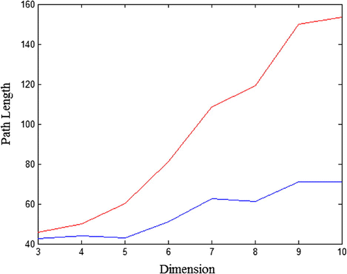
Table 1. t-test comparing two-sample means assuming unequal variances

	Our model	Taxi cab	Our model	Taxi cab	Our model	Taxi cab	Our model	Taxi cab	Our model	Taxi cab	Our model	Taxi cab	Our model	Taxi cab	Our model	Taxi cab
Number of dimensions, N	3		4		5		6		7		8		9		10
Mean	20.93862	34.93827	23.35963	44.82189	30.77087	64.63505	31.48362	70.73726	33.15113	80.77579	36.25605	95.22656	44.04183	120.05740	45.05846	129.13449
Variance	8.95179	26.93933	8.48219	34.59699	9.29186	48.52152	9.60648	59.12667	9.28532	67.12714	9.24559	73.98648	8.54108	78.80764	8.43162	85.23501
Observations	100	100	100	100	100	100	100	100	100	100	100	100	100	100	100	100
Hypothesized mean difference	0		0		0		0		0		0		0		0
df	158		145		136		130		126		123		120		118
t stat	$-23.36812$		$-32.69954$		$-44.53757$		$-47.34747$		$-54.48159$		$-64.63824$		$-81.33440$		$-86.87199$
$p(T<=t)$ one-tail	1.93908E-53		4.29807E-69		2.77319E-83		3.81589E-84		9.48758E-90		4.21973E-97		4.1093E-107		4.198E-109
t critical one-tail	1.65455		1.65543		1.65613		1.65666		1.65704		1.65734		1.65765		1.65787
$p(T<=t)$ two-tail	3.87817E-53		8.59613E-69		5.54638E-83		7.63179E-84		1.89752E-89		8.43946E-97		8.2186E-107		8.396E-109
t critical two-tail	1.97509		1.97646		1.97756		1.97838		1.97897		1.97944		1.97993		1.98027

Note that using our approach potentially allows for a more accurate estimation of sequence dependent setup times. In a relatively short time our algorithm can provide a (close to) minimal change-over time between any two configurations.

To summarize, in this note we complement the focus given to minimizing and accounting for change-over (and setup) times, by illustrating another facet of this issue, which we find relevant for LEAN manufacturing products—especially, minimizing setup and change over times—in the process industry. We show the potential that lies in introduction of readily available minimal path approaches which account for feasibility constraints, to quickly estimate minimal change-over times, while providing a detailed roadmap of how to achieve this minimal time. Future research into this prospect includes implementing our approach into manufacturing control systems, and further analysis on how these can be used to improve scheduling of multiple jobs at a production facility.

Supplementary material

Supplementary material for this article can be accessed here https://doi.org/10.1080/23311916.2017.1330911.

Additional information

Funding

The authors received no direct funding for this research.

Notes on contributors

Dror Hermel

Dror Hermel is a faculty member at Ariel’s IE&M department and conducts research in the general area of operations management. Specifically, his interest lie in adopting novel approaches from other disciplines and adapting them to improve manufacturing and service operations.

Oded Medina

Oded Medina recently completed his PhD conducting research on biologically inspired robots at the K&CG lab at Ariel University. One of his research projects dealt with real-time path planning when there are obstacles, and was adopted as a basis for the model presented in this paper.

Nir Shvalb

Nir Shvalb is heads the K&CG lab at Ariel University. His interests lie in theoretical robotics, using algebraic topology to investigate configuration spaces. This work showcases an adaptation of his works on global path planning to the domain of operations management.

References

- Allahverdi, A., Gupta, J. N., & Aldowaisan, T. (1999). A review of scheduling research involving setup considerations. Omega, 27, 219–239.
- Allahverdi, A., Ng, C., Cheng, T., & Kovalyov, M. Y. (2008). A survey of scheduling problems with setup times or costs. European Journal of Operational Research, 187, 985–1032.
- Allahverdi, A., & Soroush, H. (2008). The significance of reducing setup times/setup costs. European Journal of Operational Research, 187, 978–984.
- Baker, K. R., & Trietsch, D. (2013). Principles of sequencing and scheduling. New York, NY: John Wiley & Sons.
- Blanc, D., & Shvalb, N. (2012). Generic singular configurations of linkages. Topology and its Applications, 159, 877–890.
- Cakmakci, M., & Karasu, M. K. (2006). Set-up time reduction process and integrated predetermined time system mtm-uas: A study of application in a large size company of automobile industry. The International Journal of Advanced Manufacturing Technology, 33, 334–344.
- Leon, V. J., & Peters, B. A. (1996). Replanning and analysis of partial setup strategies in printed circuit board assembly systems. International Journal of Flexible Manufacturing Systems, 8, 389–411.
- Panwar, A., Nepal, B. P., Jain, R., & Rathore, A. P. S. (2015). On the adoption of lean manufacturing principles in process industries. Production Planning & Control, 26, 564–587.
- Shinde, S., Jahagirdar, S., Sane, S., & Karandikar, V. (2014). Set-up time reduction of a manufacturing line using smed technique. International Journal of Advanced Industrial Engineering, 2, 50–53.
- Shingo, S. (1985). A revolution in manufacturing: The SMED system. New York, NY: Productivity Press.
- Shvalb, N., Moshe, B. B., & Medina, O. (2013). A real-time motion planning algorithm for a hyper-redundant set of mechanisms. Robotica, 31, 1327–1335.
- Smed, J., Salonen, K., Johnsson, M., Johtela, T., & Nevalainen, O. S. (2003). Grouping pcbs with minimum feeder changes. International Journal of Flexible Manufacturing Systems, 15, 19–35.
- Stadnicka, D. (2015). Setup analysis: Combining smed with other tools. Management and Production Engineering Review, 6, 36–50.