Determining the volumetric characteristics of a passive linear electro-magnetic damper for vehicle applications

Abstract

Previous research has shown that passive electromagnetic damping could be feasible for automotive applications, but there would be a severe weight penalty, particularly in light weight vehicles. With modern advances in permanent magnets the feasibility of passive electromagnetic dampers is re-examined. A model of a permanent magnet and coil system is developed and validated in small scale. This magnet model is used to model a dynamic damper system which is again tested. This dynamic model is then scaled up to a two degree of freedom system to determine the damping for a quarter car model. Two damper designs are created each of which would produce a damping coefficient of 1,600 Ns/m. The proposed dampers require more than three times the volume of the equivalent hydraulic dampers.

Keywords:

• electromagnetic
• damper
• suspension

Public Interest Statement

Shock absorbers are an important component of a cars suspension system. A well designed suspension system is essential for the safety of a vehicles occupants. Most modern vehicles use suspension system designs that date back at least 50 years. An investigation is conducted to see if an electromagnetic damper system can achieve the performance required for use in modern vehicles, with a particular focus on modern lightweight electric cars. A small scale mathematical model of the cars motion and the electromagnetic damper are created and then tested to see if they are valid. The model is then scaled up to model larger dampers for a practical automobile system. It is shown that electromagnetic dampers that develop sufficient forces for realistic use are heavier than the equivalent commercial dampers.

1. Introduction

In automotive applications common oil dampers have been developed to a high level. However oil dampers provide less benefit for lightweight vehicles. Due to these and other reasons, research has turned to investigating alternative technologies for damping applications. Karnopp (1989) suggested that it is feasible to build linear electro-magnetic (e.m.) dampers for use in vehicle suspensions. The advantages of such a damper included low static friction and the fast control speed of the damper in active and semi-active applications.

Mechanically, the simplest e.m. damper uses eddy current damping. This causes the kinetic energy of motion to be converted to heat through eddy currents being formed in a material with a low, but non-zero, resistance. Eddy current damping has been proposed in vehicles (Ebrahimi, Khamesee, & Golnaraghi, 2008a, 2008b; Sodana, Bae, Inman, & Belvin, 2008), as well as buildings (Bae, Hwang, Kwag, Park, & Inman, 2014) and other structures. Such a damper is fully passive and no controllers are required.

With more advanced designed it is possible for an e.m. damper to be active, semi active, passive or a combination there of. In e.m. dampers that use a coil of wire in the magnetic field, there is the possibility of using one or more control strategies. Research in the field of e.m. dampers include (Asadi, Ribeiro, Behrad Khamesee, & Khajepour, 2015; Gupta, Jendrzejczyk, Mulcahy, & Hull, 2007; Kawamoto, Suda, Inoue, & Kondo, 2007; Montazeri-Gh & Kavianipour, 2014). Such dampers can be used entirely passively (Karnopp, 1989) or use semi active control algorithms such as Sky-Hook damping (Karnopp, Crosby, & Harwood, 1974). By the addition of energy into the system fully active suspension is also possible. The primary advantage suggested for an electromagnetic damper acting as an active element in a suspension element, is that not only can it remove energy from the system, but it could also introduce energy, usually in a very short time frame.

The use of a regenerative EM damper for the generation of power for use in car systems has also been proposed. While the power regenerated is small relative to the total overall power demands of an automobile, this power could be used for the operation of the damper itself, for supplying electrical energy to auxiliary systems in the automobile or for more efficient propulsion of the vehicle (Graves, Iovenitti, & Toncich, 2000; Guo et al., 2016; Li, Zuo, Luhrs, Lin, & Qin, 2013; Kim & Okada, 2002; Satpute, Singh, & Sawant, 2014; Zuo, Scully, & Shestani, 2010).

The concept of passive electromagnetic damping is well known and is based on Faraday’s law. Taking the case of a single cylindrical magnet and a coil of wire, damping can be achieved as is characterized in (Agutu, 2007). Unlike conventional dampers, the damping is dependant upon not only the velocity of the magnet relative to the coil, but also their relative positions.

Karnopp (1989) proposed a damper that had a magnetic field that was constant over the range of motion of the damper. Due the magnetic field being constant, the forces generated by the EM damper could be modelled by (1),(1) $$F=\frac{B^2{M}_c}{\mathit{\sigma }\mathit{\rho }}v$$(1)

The number of loops of wire in the coil will affect the force generated by the damper. However, while a fine wire will produce many more loops of wire, the reduced diameter of the wire and the extra length of the wire will produce a greater resistance. The extra resistance of a finer wire cancels out any increase in force produced by the increase in the number of loops in the coil. Therefore the force generated by Karnopp’s (1989) proposed damper is not dependant upon the number of windings used in the coil, rather the mass of the copper is the main determinant. Karnopp was limited in the force generated due to the strength of the then available permanent magnets. As can be seen in (1) the force generated by the damper is a function of the magnetic field squared, thus the increase in magnetic field strengths using modern Neodymium magnets can produce an appreciable increase in the force generated.

While research into electromagnetic damping for automotive applications has continued, the use of a simple coil/permanent magnet damper is not well modelled for this application. This is in part due to the difficulty in modelling the non-linear nature of the magnetic field produced by a coil/ magnet damper. The model to be developed for research into this field is required to determine the damping forces for an electro-magnetic damper in passive, semi-active and fully active modes as well as determining the voltage and power generated in regenerative damping mode. The complete model should be able to be used in the initial modelling stage as well as with hardware in the loop controllers for development and for practical application.

For the construction of a complete model, two separate components are required: The first element being a model of the magnetic field generated and the second is the model of the damper using the generated field. For a passive e.m. damper both the internal and external fields of the magnet have to be determined. In the determination of the near field and internal field of a cylindrical magnet there are several methods that are used.

Analytically the field can be modelled using the Coulombic model (Ravaud, Lemarquand, Babic, Lemarquand, & Akyel, 2010), the Amperian Current Model (Compter, Jansssen, & Lomonova, 2010; Ravaud et al., 2010), The Surface Charge Method (Rovers, Jansen, & Lomonova, 2010), using Maxwell’s Equations (Pfister & Perriard, 2011; Smeets, Overboom, Jansen, & Lomonova, 2011) and using the Biot-Savart equations (Babic & Akyel, 2012). The major impediment to an analytical solution is the requirement to use elliptical integrals. While the use of these integrals in many of the above approaches prohibits a complete analytical solution, these problems can be solved using modern numerical methods.

A common numerical approach is the use of the Finite Element Method (FEM) of analysis. This approach typically determines the magnetostatic field using Maxwell’s equations of electromagnetism (Zienkiewicz, Taylor, & Zhu, 2005) and has been used in cases such as in (Mahmoudi, Kahourzade, Rahim, & Hew, 2013; Kazan & Onat, 2011). In typical applications a high degree of non-linearity of the field can exist and the solution to such problems generally uses an iterative approach in which a sequence of linearised problems are solved.

Another numerical approach is the modelling of a cylindrical magnet as an air cored solenoid. This concept is well known and allows the magnet and the damper to be each modelled as current carrying loops. The Lorentz force between the magnet and the coil can then be determined is used using the Biot-Savart law (Ziolkowski & Brauer, 2010), by determining the mutual inductance (Akyel, Babic, & Kincic, 2002; Akyel, Babic, & Mahmoudi, 2009; Babic & Akyel, 2008a) or using the filament method (Babic & Akyel, 2008b).

In this work a static model of the magnetic field can be created in Matlab, the magnet being modelled as an air cored solenoid and the Biot-Savart law being used to determine the magnetic field at any point. Matlab solvers are used to obtain a solution for the elliptical integrals. To determine the flux within the damper coil at any point, the magnetic field is then integrated from the z axis to coil radius and integrated along the damper coil’s length.

A dynamic model of the damper is created in VisSim. This is a visual block diagram language that is used for the numerical simulation of dynamic systems. The VisSim model is used to simulate the behaviour of a one degree or two degree of freedom system with a passive e.m. damper. This model is required to be validated and then the model can be scaled to determine the size of the damper required for use in a light weight vehicle. The specific volumetric damping is then compared to determine if the damper is suitable for use in modern automobiles.

2. Theory of the magnetic field

Faraday’s law is used to determine the forces generated by the damper and the standard description of a damped system for the acceleration, velocity and displacement of the sprung mass. The magnet is modelled numerically as an air cored solenoid and the flux generated by the magnet is determined over the range of displacement for the masses. This is recorded as a lookup table for use in the dynamic model.

Faraday’s law was first described independently by Michael Faraday and Joseph Henry in 1831. It is given as (2),(2) $$V=\frac{d\mathrm{\Phi }}{\text{d}t}$$(2)

where the magnetic flux is dependent upon the geometry of the magnet and the relative position of the magnet and the coil. The power generated by the coil is given by (3) and (4).

(3) $$P=\frac{V^2}{R}$$(3)

(4) $$P=-\frac{1}{R}{\left(\frac{d\mathrm{\Phi }}{dt}\right)}^2$$(4)

While the force generated by the coil at any instant is (5). Substituting (4) into (5) gives (6)

(5) $$F_D=\frac{P}{v}$$(5)

(6) $$F_D=-\frac{1}{vR}{\left(\frac{d\mathrm{\Phi }}{dt}\right)}^2$$(6)

This force is then applied to the magnet/coil system.

The magnet/coil system is modelled as a single degree of freedom system with the motion along the z axis. The coil is fixed and the magnet is free to move, while attached to a spring. The magnet and coil provided a damping force for this system. A freely vibrating damped system is described by (7)

(7) $$m\ddot{z}+c\dot{z}+kz=0$$(7)

In the case of a single magnet and coil the force of the damping is dependant upon both the velocity and position. This is now described as (8)

(8) $$m\ddot{z}+\frac{1}{R\dot{z}}{\left(\frac{d\mathrm{\Phi }}{dt}\right)}^2+kz=0$$(8)

For this equation to be complete, two additional terms are required: F_C, to represent the Coulombic damping. And c_nat to represent the natural damping of the system, the complete equation for the electro-magnetic damper is given as (9).(9) $$m\ddot{z}+\frac{1}{R\dot{z}}{\left(\frac{d\mathrm{\Phi }}{dt}\right)}^2+c_{\text{nat}}z+kz+F_C=0$$(9)

The magnet is modelled as an air cored solenoid with a finite number of loops. The magnetic field is then generated for each loop of wire with a current flowing through it. The superposition principle is then used at each point measured to sum the magnetic field from each loop in the solenoid to produce the total magnetic field.

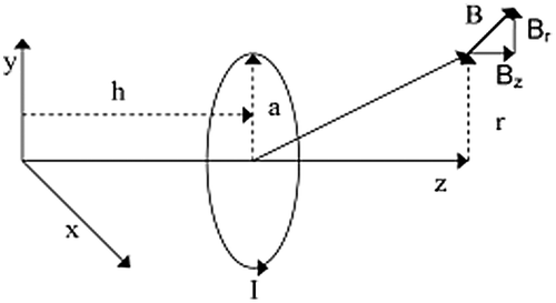
For a single loop as shown in Figure 1, using the Biot-Savart law of Magnetostatics, (Kuns (2007) derives the magnetic field at any point is space as (10),(10) $$B(r,z)=\frac{{\mathit{\mu }}_{o}Ik}{4\mathit{\pi }\sqrt{a{r}^3}}\left[-(z-h)\left(K-\frac{2-k^2}{2(1-k^2)}E\right)\widehat{r}-r\left(K+\frac{k^2(r+a)-2r}{2r(1-k^2)}E\right)\widehat{z}\right]$$(10)

Figure 1. The determination of the z and r components of a magnetic field at a point, generated by a current loop using the Biot-Savart law.

using polar coordinates where the loop is centred on the z axis, with the loop on the r axis. The complete elliptical integrals of the first and second kind are both with regards to k² in the form K(k²) and E(k²), where k is given by (11).

(11) $$k=\sqrt{\frac{4ar}{{\left(r+a\right)}^2+{(z-h)}^2}}$$(11)

In determining the change in flux, only the z component of the field is required and is given by (12).(12) $$B(z,r)=\frac{{\mathit{\mu }}_{o}Ik}{4\mathit{\pi }\sqrt{a{r}^3}}r\left(K+\frac{k^2(r+a)-2r}{2r(1-k^2)}E\right)\widehat{z}$$(12)

For the complete model of a coil-magnet system, the coil is modelled as a solenoid with multiple loops and the permanent magnet is also modelled as a solenoid with multiple loops. The flux through each loop of the coil is calculated by (13).

(13) $$\mathrm{\Phi }=\sum _1^N\sum _1^n\left({\int }_0^{r}B(z,r)\widehat{z}dr\right)$$(13)

Substituting (13) into (9) gives a complete numerical model of the passive damper.

3. The dynamic damper model

To describe the magnet, the magnetic flux along the z axis is modelled using (13). This is then used to determine the enclosed flux of a coil along the axis of motion for a distance of 60 in 1 mm increments. Symmetry about the centre of the coil is used along the axis of motion to reduce the calculation times in modelling the flux on each side to the magnet. The magnetic field and fluxes are determined using the functional language MATLAB. These modelled fluxes are then formed into a lookup table using linear interpolation for use in the dynamic damper simulation.

The dynamic damper model is created in the numerical modelling package VisSim, as (10). The flux at any position is determined from the look up table with a linear interpolation. Factors for Coulombic and natural viscous damping are included.

The model is then given a step input and the subsequent displacements of the spring–damper system are then compared to the measured displacements of an electromagnetic damper. The damping coefficient of the total system is then determined. From this and the measured natural damping of the system, the damping coefficient of the damper is determined.

For the dynamic simulation of a one degree of freedom system, Equation (14(14) $$k{(z_1-z_0)}_{}{+}_{}c({\dot{z}}_1-{\dot{z}}_0)+m{\ddot{z}}_{}{=}_{}0$$(14) ) is developed in VISSIM.(14) $$k{(z_1-z_0)}_{}{+}_{}c({\dot{z}}_1-{\dot{z}}_0)+m{\ddot{z}}_{}{=}_{}0$$(14)

where k is the spring constant, z₁ is the position of the sprung mass, z₀ is the position of the road surface, c is the damping coefficient and m is the sprung mass in kg. To this is added a term, c_nat, for the natural damping efficient, which is the damping of the system without the damper, F_C which is the Coulombic damping and F_D which is the force exerted by the passive electromagnetic damper. This gives (15)(15) $$k(z_1-z_0)+c_{nat}({\dot{z}}_1+{\dot{z}}_0)+m\ddot{z}+F_C+F_D=0$$(15)

4. Materials

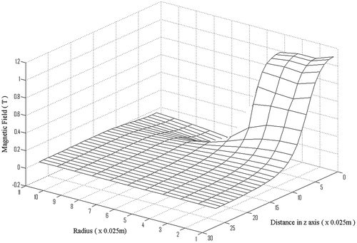
The magnet chosen to model is a neodymium rare earth magnet rated as an N35, it is 0.028 m long and 0.0095 meters in radius with a pole strength of 0.5778 T. A computer model of the magnetic field is created in MATLAB Simulink. The modelled field produced is shown in Figure 2. The North/South poles are along the z axis. The figure shows one quarter of the magnet field of the magnet measured from the centre. The field is rotationally symmetrical and the poles are also symmetrical. The magnetic field of the prototype magnet was measured at 2.5 mm intervals using an Alphalab Model 1 DC Magnetometer.

Figure 2. The modelled magnetic field of a Neodymium magnet. The North/South poles of the magnet are mounted along the z axis.

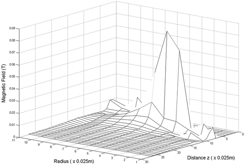
The absolute differences between the measured and modelled values are represented in Figure 3. For majority of the region modelled the difference between the modelled field and the measuredl field is less than 0.01 T. The largest differences between measured and modelled results occur where the magnetic field is changing the fastest and where the field is the strongest. The average error between the measured and modelled fields is 3.5%. When the differences are averaged over the entire field, the measured field readings are 1.1% larger than the predicted values. The largest absolute difference between the measured and modelled field occurs at the physical pole of the magnet where the limitations of the measuring equipment are observed. Even small differences in displacement, such as the thickness of the magnetic probe, make a significant difference to the results. This method of testing only measures the external field of the magnet and cannot measure the internal component of the magnetic field. The peak magnetic field strength is physically inside the magnet and drops off in a non-linear manner with distance from the poles.

Figure 3. The absolute difference between modelled and measured magnetic field.

The component of the magnetic field physically inside the magnet represents the major component of any flux that will be used in the model, therefore an independent method is required to test for the internal field. By using the modelled field, the flux of the magnet travelling through a coil is determined. By passing a magnet through the prototype of the modelled coil, a voltage is produced. This is measured and converted to an electromotive force for calculations. The rate of change of flux is then determined from this as in Figure 4.

Figure 4. Change in flux of magnet passing through a coil.

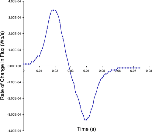
Summing over time the total flux of the magnet in the coil is determined to be 0.004501 Wb. Summing the model flux of the damper/coil system gave a modelled flux of 0.00488 Wb. There is an agreement between the modelled and measured data of 92.2%.

5. Vibration analysis

A small test rig was constructed for initial validation of the damper model as shown in Figure 5. This is adjustable in all three axes to ensure that the magnet does not mechanically interact with the coil. The damper itself consists of 120 turns of 1 mm copper wire wound as three layers of 40 turns each, wound onto a PVC core. An accelerometer is attached to the sprung mass and data is recorded with a Signal Analyser.

Figure 5. A small scale test rig with signal analyser. (1) is the spring, (2) the coil, (3) is a mass attached to the magnet, which is inside the coil. These are then connected to the spring. The accelerometer (4) is connected to the signal analyser (5).

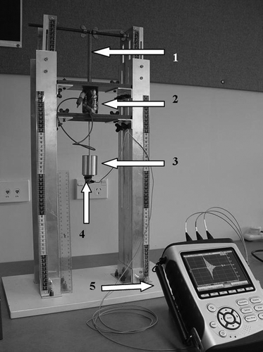
A series of trials are conducted with the weight of the damper and hanger of 100 g plus additional weights of 300–1,000 g. A series of runs is also conducted with the damper in place but without damping being applied. These data runs are used to determine the natural damping and the Coulombic damping of the system.

5.1. In the time domain

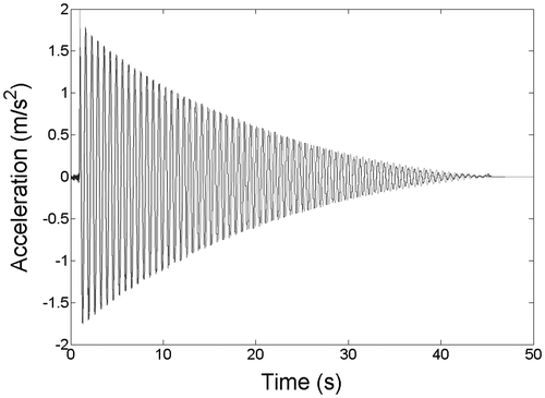
To determine the Coulombic Friction and the natural damping of the system, a run of the physical system being modelled is conducted. During modelling, visual inspection of the acceleration-time graphs for the model and for the recorded data is used to determine these values so as to produce a displacement-time graph that matches a known experimental result for the rig being used. The combined graph for the natural damping coefficient and the Coulombic Damping factor for an added weight of 1 kg are determined as in Figure 6. For the values given, the two graphs merge to the point where there are almost indistinguishable from each other. This process is repeated for every weight that is used during the experimentation.

Figure 6. The modelled and measured accelerations for an undamped 1,100 g mass.

Note: The dashed line are the theoretical values and the solid line are the experimental values.

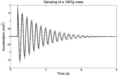
A series of runs is conducted using added weights from 300–1,000 g. A typical result is shown in Figure 7. This represents an added weight of 1,000 grams and the magnet is modelled as a solenoid with a current of 30.4 Amps. As can be noted, there is a difference of magnitude between the predicted and modelled acceleration. This is consistent in all readings and is a systematic uncertainty caused by calibration issues and resolution in numerical modelling.

Figure 7. The modelled and measured acceleration of a damped 1,100 g mass. Natural damping = 0.1 Ns/m and Coulombic damping = 0.0024 Ns/m.

Note: The dashed line are the theoretical values and the solid line are the experimental values.

The damping coefficient of the total damper for various weights is given in Table 1 The relative agreement between the modelled and measured data is also given in Table 1. This showed an agreement between the modelled and the measured damping of the magnet-coil damper system to be between 75–93%. The mean agreement is 84%.

Table 1. The modelled and actual damping of the small scale prototype damper for a step input

Mass (g)	Damper modelled (Ns/m )	Damper actual (Ns/m )	Agreement (%)
1,097	0.5786	0.6416	90.2
997	0.5223	0.4833	92.5
897	0.5973	0.6884	86.8
797	0.5672	0.7047	80
697	0.5993	0.7872	76.1
597	0.6327	0.8776	72.1
497	0.6083	0.8183	74.3
397	0.7333	0.6597	111.2

5.2. In the frequency domain

To determine the effectiveness of the passive e.m. damper and to verify the accuracy of the modelled passive damper, the passive damper was tested at frequencies from below the resonant frequency of the system to approximately 9 Hz. The upper frequency was limited by the experimental apparatus. A series of experimental runs are conducted over the frequency range with a pseudo-sinusoidal input and compared to the theoretical model. The magnet used is the same 29 mm long neodymium magnet that was previously modelled. The coil is the single coil as described previously. The frequency of the VisSim model is set at 1,000 Hz to avoid any aliasing effects and to reduce numerical errors.

A comparison is conducted between the measured damped motion of the system and the modelled damped motion of the system. The results are given in Figures 8 and 9. The values displayed are the absolute r.m.s. velocity of the damper at the various frequencies for experimental runs of over 30 s.

Figure 8. Comparison of the modelled and actual passively damped motion in the frequency domain. “——” actual measurements and “- - - -” are the modelled values.

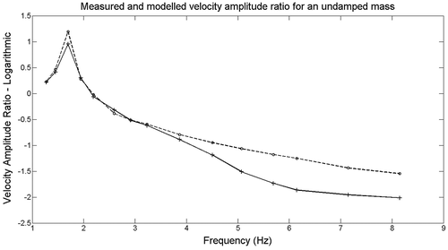
Figure 9. A comparison of the modelled and actual damped velocity amplitude ratio of the undamped mass in the frequency domain.“——” actual measurements and “- - - -” are the modelled values.

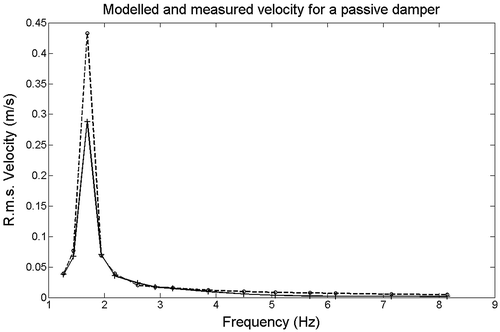
At the near resonant frequency of 1.58 Hz the modelled displacement and velocity increased by several factors. The physical prototype has a limited allowable range of motion and therefore is much more limited in both displacement and velocity. At frequencies over 4–5 Hz the accelerometer drift of the measuring accelerometer, when integrated, can become larger than the actual velocity measurements. In the range of 1–4 Hz there is a better than 93% agreement between the measured and modelled values. However, for frequencies above 4 Hz the agreement drops rapidly to 38%. This drop in accuracy is caused by accelerometer drift creating a larger noise than the signal that is being measured. These effects are noted for both the damped and undamped motion. In the case of higher frequencies the relative performance of the damped and undamped systems are compared, rather than the absolute values.

While the passive damper is sufficient to produce observable damping effects, the magnitude of this damping is designed for research purposes and not practical damping applications. To determine if this damper is of practical use, a larger scale model is required.

5.3. The small scale model

In this model the total mass of 500 g mass represents the lower mass limit of the system. Below this point the model no longer fully represents the damper/mass system as the relative uncertainties accumulate. In all cases the predicted damping is less than the recorded damping. As is observed in Figure 8, there are some calibration issues between recorded data and the model. This should produce a slightly higher than predicted damping factor. It is also noted that the coil is wound onto a paramagnetic substance. This property is not included in the model. This should again mean that the model predicts a lesser value. A further assumption is the axisymmetric nature of the field within the magnet; this is observed to be not fully accurate. The resistance of the coil is important in the final force generated. The resistance of the coil is accounted for, but the reactance of a coil of a coil for an alternating current caused by the magnet is not modelled. An analysis of the reactance of the coil produced a difference of less than 0.1% for the impedance of the coil. From testing the system showed sensitivity to the initial conditions and the measurement with of the total mass of 1,000 g show some of this sensitivity in the result. Resolution issues due the scale of this experiment are apparent during testing. Any disparity between the model and measured will cascade as the dynamic model is modelled using the solutions produced by the static model. The static model showed a greater than 90% agreement and the total model produced a, average agreement of 84%.

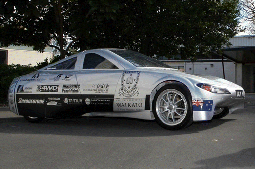
Having good confidence in the validated model, it was then applied to a full size, lightweight electric vehicle as shown in Figure 10. The magnetic force, F_D, was calculated from Equation (6). A two degree of freedom model was simulated with F_D, being varied until it produce a typical damped response for the spring mass. This was an iterative approach that gave the parameters for number of coils, magnets and windings. This is explained in detail in Section 6.

Figure 10. University of Waikato Ultracommuter battery electric vehicle.

6. Scaling up the passive e.m. damper for a lightweight vehicle

To determine the feasibility of the passive electromagnetic damper as a component for full size automobiles a two degree of freedom model of a car suspension system is created.

For a quarter car, the masses could be modelled as a two degree of freedom as in Figure 11, where m₁ is the unsprung mass/tyre, m₂ is the sprung mass/car body, z₀ is the displacement of the road surface, z₁ is the displacement of the unsprung mass, z₂ is the displacement to the sprung mass, k₁ is the tyre stiffness, k₂ is the shock absorber spring stiffness, c is the damping coefficient of the tyre and F_D is the damper force. For a two degree of freedom system the equations of the displacement of the unsprung and sprung masses are given by (16) and (17).(16) $$m_1{\ddot{z}}_1+k_1(z_1-z_0)-c({\dot{z}}_1-{\dot{z}}_0)+k_2(z_2-z_1)+F_D=0$$(16) (17) $$m_2{\ddot{z}}_2+k_2(z_2-z_1)-F_D=0$$(17)

Figure 11. A two degree of freedom suspension system.

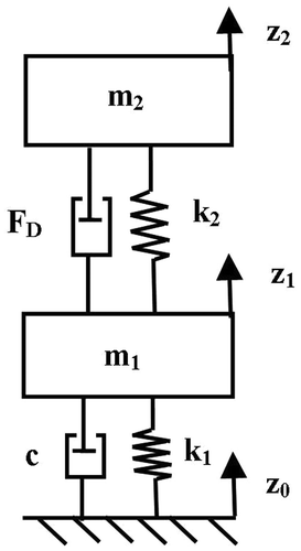
As the damping from tyres are usually considered negligible the equations simplified to (18) and (17).(18) $$m_1{\ddot{z}}_1+k_1(z_1-z_0)+k_2(z_2-z_1)+F_D=0$$(18) (17) $$m_2{\ddot{z}}_2+k_2(z_2-z_1)-F_D=0$$(17)

This is modelled in VisSim for a light weight electric vehicle similar to the University of Waikato Ultracommuter electric vehicle as shown in Figure 10 and using values as given in Table 2. These values give a resonant frequency of the sprung mass is 1.322 Hz and the frequency of the tyre “hop” is 10.41 Hz.

Table 2. Values for a two degree of freedom quarter car system for the University of Waikato Ultracommuter automobile

Properties	Value
Sprung mass	200 kg
Unsprung mass	25 kg
Spring stiffness	12,500 N/m
Tyre stiffness	100,000 N/m

A pair of larger magnets is modelled for suitability for use in a more powerful damper. Both are cylindrical and axially magnetised. Each of these magnets are matched with a coil the same length as the magnet and consisting of a single layer of wire. The properties of the magnets and their responding coils are given in Table 3.

Table 3. Values for two magnets and two coils

	ND3522	ND5550
Property–Magnet
Diameter (mm)	35	55
Length (mm)	22	50
Mass (kg)	0.074	0.4153
Field strength at pole (T)	0.5791	0.5783
Property–Coil
Length (mm)	22	60
Radius (mm)	20	30
Turns	22	50
Wire diameter (mm)	1	1.2
Mass coil (kg)	0.0194	0.0953
Resistance coil (Ω)	0.0563	0.14

For the damper to be effective, a damping ratio of 0.5 should be the minimum achievable figure. This requires a damping coefficient of 1,600 Ns/m. For a single coil and magnet the maximum damping coefficient achieved for the ND3522 magnet is 4.60 Ns/m and for the ND5550 the maximum achieved is 20.9 Ns/m. The weight of the magnet-coil system is 0.0934 kg for the ND3522 and 0.5106 kg for the ND5550. With the masses and spring stiffnesses involved a single magnet and coil of the types in Table 3 achieved only a small percentage of the required damping coefficient.

To increase the performance the number of layers is increased to five. This increased the damping effect for the ND3522 to 23.5 Ns//m and for the larger ND5550, 106.3 Ns/m. The masses of the coil-magnet systems increased to 0.171 and 0.892 kg respectively. These damping coefficients remained insufficient to give the suspension system the required damping ratio.

The damping force is further increased by using a second coil with an opposing direction as illustrated in Figure 12(a). This second coil is wound in the opposite direction to the first coil and has a reversed polarity. This provides approximately twice the damping of the single magnet coil system, but without the requirement of adding a second magnet, only a second coil. For a single magnet and two matched coils, as in Table 3, each of five layers, the damping increased to 47.6 and 211.8 Ns/m.

Figure 12. Two damper systems with multiple magnets and coils. (a) A magnet and two coil damper system and (b) A multi-magnet and multi-coil damper.

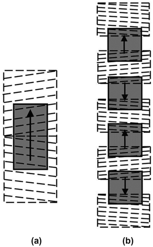
Still greater damping coefficients are obtained through the use of a stack of magnets and coils of opposing magnetic fields and polarities as illustrated in Figure 12(b). In (Fow & Duke, 2016) two magnet/coil stacks were proposed, each of which acted as a two phase linear electromagnetic generator. These were both designed to produce a damping coefficient of approximately 1,600 Ns/m. The specifications of these dampers are given in Table 4.

Table 4. Passive e.m. damper properties to achieve a damping coefficient of 1,600 Ns/m

Magnet	ND3522	ND5550
Number of magnets	17	8
Number of coils	18	9
Number of layers	10	5
Damping coefficient (Ns/m)	1,581	1,638
Mass (kg)	4.75	7.61

A major consideration in any damper design is the physical space that the damper occupies. A damper made from ND3522 magnets and coils produces a stack 770 mm tall, without any mounting and 920 mm tall at maximum extension. The volume of this stack is 2.177 litres. For a damper stack made from the ND5550 magnet-coil combination, the height is 800 mm minimum and 950 mm at maximum extension. The volume of the second proposed damper is 3.078 litres. This is compared to a equivalent commercial damper that is 550 mm long at full extension and with all of the mountings. The dash pot on a hydraulic damper will produce a specific volumetric damping of over 2,000 Ns/m per litre of volume. While the passive dampers produce specific volumetric damping of 756 and 532 Ns/m per litre respectively. In the case where the volume of the damper is important, an electromagnetic damper is not only heavier than the equivalent oil damper, but occupies significantly more space and has extra complexity.

7. Conclusions

Both the model of the magnet and the model of the dynamic system are validated. The model of the magnet producing a better than 96% agreement between the modelled and measured magnetic fields. This produced a 92% agreement between the modelled and measured flux generated by the magnet-coil model. Testing of the single degree of freedom damper model produced 83% agreement in the time domain and 94% agreement for the frequency domain, where the measured signal is sufficient for reliable measurements.

The model was then scaled up to produce two proposed dampers, each of which would produce a damping coefficient of 1,600 Ns/m, which is considered sufficient for the damping of a lightweight vehicle. The two dampers occupied three to four times the volume of an equivalent hydraulic damper when sans covers, connecting rods, other damper “furniture” or any systems to remove the heat generated by the damper. It is therefore determined that there is no volumetric advantage in the use of the proposed damper in a purely passive mode. Further research should be conducted to determine if the damper in semi-active or regenerative modes would justify the increased weight and volume of the passive e.m. damper.

Funding

The authors received no direct funding for this research.

Nomenclature
a	=	Radius of loop (m)
B	=	Magnetic Field (T)
Br	=	Radial component of Magnetic Field (T)
Bz	=	Parallel component of Magnetic Field (T)
c	=	Damping coefficient (N s/m)
cn	=	Natural damping (N s/m)
E	=	Complete elliptical integral of the second kind
FC	=	Coulombic damping (N)
FD	=	Damper force (N)
h	=	Loop displacment (m)
I	=	Current (A)
K	=	Complete elliptical integral of the first kind
k	=	Spring constant (N/m)
k	=	Constant
lm	=	Length of magnet (m)
m	=	Mass (kg)
Mc	=	Mass of conductor (kg)
N	=	Number of loops in magnet
n	=	Number of loops in the coil
P	=	Power (W)
Ps	=	Pole Strength (T)
R	=	Resistance(Ω)
r	=	Distance from z axis (m)
t	=	Time (s)
V	=	Voltage (V)
v	=	Velocity (m/s)
x	=	Displacement x axis (m)
y	=	Displacement y axis (m)
z	=	Displacement z axis (m)
μ0	=	Permeability of free space = 4π × 10−7 (H/m)
ρ	=	Density (kg/m3)
σ	=	Resistivity (Ωm)
Φ	=	Flux (Wb)

Additional information

Notes on contributors

A. Fow

A. Fow is a Teaching Fellow in the School of Engineering at the University of Waikato. His main area of research is the use of active, passive and semi-active electromagnetic dampers (EM) in vehicles. The research involves mathematical modelling and the use of software, such as Matlab and VisSim to develop numerical solutions. He uses experimentation to validate his solutions and is a strong advocate of “real-time” control for rapid and flexible control system development. The fundamental EM work is now being developed for electric powered agricultural vehicles with full scale testing about to be undertaken.

References

- Agutu, W. O. (2007). Characterization of electromagnetic induction damper ( unpublished thesis (MSc)). Miami University, Oxford.
- Akyel, C., Babic, S., & Kincic, S. (2002). New and fast procedures for calculating the mutual inductance of co-axial circular coils (circular coil-disk coil). IEEE Transactions on Magnetics, 38, 2367–2369.10.1109/TMAG.2002.803576
- Akyel, C., Babic, S., & Mahmoudi, M. M. (2009). Mutual inductance calculations for non-coaxial circular air coils with paralle axes. Progress in Electromagnetics Research, 91, 287–301.10.2528/PIER09021907
- Asadi, E., Ribeiro, R., Khamesee, M. B., & Khajepour, A. (2015). A new adaptive hybrid electromagnetic damper: Modelling, optimization, and experiment. Smart Materials and Structures, 24, 075003.10.1088/0964-1726/24/7/075003
- Babic, S. I., & Akyel, C. (2008a). Calculating mutual inductance between circular coils with inclined axes in air. IEEE Transactions on Magnetics, 44, 1743–1750.10.1109/TMAG.2008.920251
- Babic, S. I., & Akyel, C. (2008b). Magnetic force calculation between thin coaxial circular coils in air. IEEE Transactions on Magnetics, 44, 445–452.10.1109/TMAG.2007.915292
- Babic, S. I., & Akyel, C. (2012). Magnetic force between inclined circular filaments placed in any desired position. IEEE Transactions on Magnetics, 48, 69–80.10.1109/TMAG.2011.2165077
- Bae, J. S., Hwang, J. H., Kwag, D. G.,Park, J., & Inman, D. J. (2014). Vibration suppression of a large beam structure using tuned mass damper and eddy current damping. Shock and Vibration, 2014.
- Compter, J. C., Jansssen, J. L. G., & Lomonova, E. A. (2010). Ampere’s circuital 3-D model for non-cuboidal magnets. IEEE Transactions on Magnetics, 46, 4009–4015.10.1109/TMAG.2010.2070804
- Ebrahimi, B., Khamesee, M. B., & Golnaraghi, F. (2008a). Design and modeling of a magnetic shock absorber based on eddy current damping effect. Journal of Sound and Vibration, 315, 875–889.10.1016/j.jsv.2008.02.022
- Ebrahimi, B., Khamesee, M. B., & Golnaraghi, F. (2008b). Eddy current damper feasibility in automobile suspension: Modeling, simulation and testing. Smart Materials and Structures, 18, 015017.10.1088/0964-1726/18/1/015017
- Fow, A., & Duke, M. (2016, April). Electromagnetic damper control strategies for light weight electric vehicles. In Advanced Motion Control (AMC), 2016 IEEE 14th International Workshop (pp. 9–15). Piscataway: IEEE.10.1109/AMC.2016.7496321
- Graves, K.E., Iovenitti, P. G., & Toncich, D. (2000). Electromagnetic regenerative damping in vehicle suspension systems. International Journal of Vehicle Design, 24, 182–197.10.1504/IJVD.2000.005181
- Guo, S., Xu, L., Liu, Y., Liu, M., Guo, X., & Zuo, L. (2016, August). Modeling, experiments, and parameter sensitivity analysis of hydraulic electromagnetic shock absorber. In ASME 2016 International Design Engineering Technical Conferences and Computers and Information in Engineering Conference (pp. V003T01A032–V003T01A032). American Society of Mechanical Engineers.
- Gupta, A., Jendrzejczyk, J. A., Mulcahy, T. M., & Hull, J. R. (2007). Design of electromagnetic shock absorbers. International Journal of Mechanics and Materials in Design, 3.3, 285–291.
- Karnopp, D. (1989). Permanent Magnet Linear Motors Used as Variable Mechanical Dampers for Vehicle Suspensions. Vehicle System Dynamics, 18, 187–200.10.1080/00423118908968918
- Karnopp, D. C., Crosby, M. J., & Harwood, R. A. (1974). Vibration control using semi-active force generators. Journal of Engineering for Industry, 96, 619–626.10.1115/1.3438373
- Kawamoto, Y., Suda, Y., Inoue, H., & Kondo, T. (2007). Modeling of electromagnetic damper for automobile suspension. Journal of System Design and Dynamics, 1, 524–535.10.1299/jsdd.1.524
- Kazan, E., & Onat, A. (2011). Modeling of air core permanent-magnet motors with a simplified nonlinear magnet analysis. IEEE Transactions on Magnetics, 47, 1753–1762.10.1109/TMAG.2011.2111375
- Kim, S. S., & Okada, Y. (2002). Variable resistance type energy regenerative damper using pulse width modulated step-up chopper. Transactions of the ASME, 124, 110–115.
- Kuns, K. (2007, August 14). Calculation of magnetic field inside plasma chamber. California: UCLA report.
- Li, Z., Zuo, L., Luhrs, G., Lin, L., & Qin, Y. X. (2013). Electromagnetic energy-harvesting shock absorbers: Design, modeling, and road tests. IEEE Transactions on Vehicular Technology, 62, 1065–1074.10.1109/TVT.2012.2229308
- Mahmoudi, A., Kahourzade, S., Rahim, N. A., & Hew, W. P. (2013). Design, analysis, and prototyping of an axial-flux permanent magnet motor based on genetic algorithm and finite-element analysis. IEEE Transactions on Magnetics, 49, 1479–1492.10.1109/TMAG.2012.2228213
- Montazeri-Gh, M., & Kavianipour, O. (2014). Investigation of the active electromagnetic suspension system considering hybrid control strategy. Proceedings of the Institution of Mechanical Engineers, Part C: Journal of Mechanical Engineering Science, 228, 1658–1669.
- Pfister, P. D., & Perriard, Y. (2011). Slotless permanent-magnet machines: General analytical field calculation. IEEE Transactions on Magnetics, 47, 1739–1752.10.1109/TMAG.2011.2113396
- Ravaud, R., Lemarquand, G., Babic, S., Lermarquand, V., & Akyel, C. (2010). Cylindrical magnets and coils: Fields, forces, and inductances. IEEE Transactions on Magnetics, 46, 3585–3590.10.1109/TMAG.2010.2049026
- Rovers, J. M. M., Jansen, J. W, & Lomonova, E. A. (2010). Analytical calculation of the force between a rectangular coil and a cuboidal permanent magnet. IEEE Transactions on Magnetics, 46, 1656–1659.10.1109/TMAG.2010.2040589
- Satpute, N. V., Singh, S., & Sawant, S. M. (2014). Energy harvesting shock absorber with electromagnetic and fluid damping. Advances in Mechanical Engineering, 6, 693592.
- Smeets, J. P. C., Overboom, T. T., Jansen, J. W., & Lomonova, E. A. (2011). Three-dimensional magnetic field modeling for coupling calculations between air-cored rectangular coils. IEEE Transactions on Magnetics, 47, 2935–2938.10.1109/TMAG.2011.2145365
- Sodana, H. A., Bae, J.-S., Inman, D. J., & Belvin, W. K. (2008). Improved concept and model of eddy current damper. Transactions of the ASME, 128, 294–302.
- Zienkiewicz, O. C., Taylor, R. L., & Zhu, J. Z. (2005). The finite element method: Its basis and fundamentals (6th ed.). Amsterdam: Elsevier.
- Ziolkowski, M., & Brauer, H. (2010). Fast computation technique of forces acting on moving permanent magnet. IEEE Transactions on Magnetics, 46, 2927–2930.10.1109/TMAG.2010.2044643
- Zuo, L., Scully, B., & Shestani, J. (2010). Design and characterization of an electromagnetic energy harvester for vehicle suspensions. Smart Materials and Structures, 19, 045003.10.1088/0964-1726/19/4/045003