Inventory decisions in a two-echelon system with remanufacturing, carbon emission, and energy effects

Abstract

In this study, we propose an inventory model consisting of a depot and a distributor with environmental and finite remanufacturing generations considerations. Investigation of the environmental effects is done by examining how carbon emissions and energy consumption for both transportation and production affect the model’s optimal solution. In the system, the depot fulfils demand at the distributor through ordering new products from outside supplier and remanufacturing used items that are returned from the market. We build the joint annual inventory cost function and find its minimum value by determining the optimal value of shipment lot size, number of shipments per year, and the number of remanufacturing generations. The results show that the proposed model gives benefit to the depot and the distributor, respectively. Optimizing the inventory related costs and the environmental costs actually provides less remanufacturing generations. In the other hand, higher amount of solid waste disposal and carbon emissions will be generated yet lower amount of energy is consumed. This study also showed that the joint total cost can be reduced by increasing the number of used items collected from the market.

Keywords:

• closed-loop supply chain
• reverse logistics
• remanufacturing
• carbon emissions
• energy effects

Public Interest Statement

Many manufacturing companies have been focusing on sustainable and green supply chain management in the last decades. Sustainable supply chain generally achieved by recovering some of end-of-life products in the market and subsequently redistribute it after being remanufactured or recovered. Whereas, a green supply chain is more concerned to minimize the environmental impacts that occur from the implementation of supply chain management. In achieving such supply chain conditions, a proper inventory planning is required. This research develops an inventory model that can assist manufacturing companies in determining the optimal number of shipments, shipment lot size, and number of remanufacturing generations, hence inventory related costs among the supply chain can be minimized. Through this research, manufacturing companies can learn how environmental issues impact the supply chain decisions in terms of shipping and remanufacturing generation.

1. Introduction

In the field of supply chain management, researchers and practitioners are currently focused on inventory and production operations management that are environmentally sustainable to increase company’s competitive advantages (Mohanty & Prakash, 2014; Sasikumar & Kannan, 2009; Srivastava, 2007). Companies are required to manage the supply chain as efficient as possible hence wastes can be minimized. One attempt to be done by the company in order to create a sustainable supply chain or green supply chain is through product take-back and recovery from the market (Heese, Cattani, Ferrer, Gilland, & Roth, 2005). This concept is often referred as Reversed Logistic (RL) or Reverse Supply Chain Management (RSCM). Sasikumar and Kannan (2008) define RSCM as a supply chain where companies usually do some tasks, including collecting of used items, used product recovery or removal and products resell and distribution. According to Jauhari, Dwicahyani, and Kurdhi (2017), product recovery is described as a set of activities to reclaim value of a product at the end of its useful life (EoL product). Nowadays, many industries need to implement the principle of returned item recovery due to some restrictions such as government regulations, social-ethical responsibilities, and economic factor in order to become a sustainable supply chain. The concept of RL itself has currently been performed by many industries such as automobiles, computers, printers, copiers, mobile phones, televisions, refrigerators, air conditioners, washing machines, tires and bulky products such as printed circuit boards (Xia, Jia, & He, 2011). Companies that have successfully implemented the RL strategy include Apple, Dell and Sony. In another case, the principle of RL has been tried out for Indian LPG agency (Yogi, 2015).

Increasing complexity of the global industry has made management of the supply chain system difficult to carry out. In the series of supply chain management, inventory control and management plays an important role hence it needs to be performed properly and collaboratively by all parties engaged in the supply chain, including manufacturing and distributing company. Jauhari, Mayangsari, Kurdhi, and Wong (2017) emphasized that a better collaboration in managing inventories across the entire supply chain may reduce total cost. A proper inventory control planning and management also allows the system to control a number of adequate materials within the chain. According to Radzuan, Othman, Anuar, and Osman (2014), ineffectiveness of inventory control may significantly affect the production operations in manufacturing environment. Russel and Taylor (2006) estimated that 30% of the total value of the inventory is the result of the average holding cost of manufacturing goods inventory held in the warehouse. As to obtain the optimal overall inventory performance in the supply chain, the company needs to determine how to control the inventory flows effectively. For this reason, the correct planning of inventory control and management becomes an important thing needs to be organized before executing a supply chain.

In the series of supply chain planning and management, environmental consideration is inevitable and needs to be elaborated (Bonney & Jaber, 2011). According to Bazan, Jaber, and El Saadany (2015), various environmental issues that may arise from supply chain activities, i.e. production and transportation, including water emission, solid waste disposal, water contamination, thermal pollution up to energy consumption. Energy consumption referred to all electrical energy needed in the remanufacturing process. From these concerns, some researchers have accommodated environmental costs in RL mathematical modelling to learn and understand how a supply chain- planning and management is done in accordance with environmental considerations.

The model developed in this study is a reverse logistic inventory model of a system that considers the integration between parties in the supply chain and investigation of carbon emissions and energy consumptions from remanufacturing and transportation operations. The system studied is the RSCM in which there is a return of used items from consumers to producers at the end of its useful life (EoL). We build the joint annual inventory cost function and find the minimum value by determining the optimal value of shipment lot size, number of shipments per year, and the number of remanufacturing generations. The paper is organized as follows. Section 2 provides a literature review of related papers which helps the readers in figuring out the novelty of the study. Problem description of the model, as well as the notations and assumptions used in the model, are presented in Section 3. Section 4 gives an explanation about the model formulation and solution procedure. The numerical example of the model is presented in Section 5. Section 6 presents the results of sensitivity analysis. Finally, conclusions and future research directions are given in Section 7.

2. Literature study

Researches and studies of inventory modelling in the field of reverse logistics have been raised in the last few decades. Due to both economic and environmental reasons, many researchers have built and developed quantitative models to analyze the corresponding system in managing product return flow (Bazan, Jaber, & Zanoni, 2016). Most of the primary studies focused mainly on the deterministic model with the traditional inventory system without considering other aspects such as integration among parties in the supply chain, correlated demand and returns, environmental factors, form of recovery, disposal of waste, and others activities that actually performed by companies. Along with the environmental conditions development and also the increasing complexity of production systems, the researchers keep on developing the inventory model on the related field, so that complexity of the real production system could be accommodated.

The first inventory model that initiated the study of product return on inventory management is the model belongs to Shcrady (1967). In his study, an EOQ model was developed for repairable items and instantaneous remanufacturing rate. The model of Scrady is then became the root of all inventory model in the field of reverse logistic (Fleischmann et al., 1997). There are numerous extensions of the model, including Nahmias and Rivera (1979), Mabini, Pintelon, and Gelders (1992), Richter (1996a, 1996b, 1997), and Fleischmann et al. (1997). Nahmias and Rivera (1979) extended the model by accommodating finite recovery rate and also storage capacity in both repair and production shops. Mabini et al. (1992) proposed inventory model with backorders. By observing the reality in the production system. Richter (1996a, 1996b) realized that some returned items may not be recovered and needs to be disposed. In his study, he proposed an EOQ model considering waste disposal activity. Then, Richter (1997) developed his previous models by doing a cost comparison analysis between pure (bang-bang) policy and mixed policy. Pure (bang-bang) policy is a policy in product returns management which the manufacturer either disposes or repairs all the used items. Besides, the mixed strategy is a policy which the manufacturer combines the two activities, disposal and repair, in order to manage the used items.

In the context of logistics and inventory management system, one aspect that should not be put a side is integration between other parties in the supply chain system. According to Jauhari, Pamuji, and Rosyidi (2014), a traditional single-state system inventory management was not suitable for managing inventories across the chain. Consequently, in order to control the balance of the system as well as to reduce cost along with environmental effects, management of forward and reverse logistics should be done along the chain. The supply chain that manages forward as well as reverse logistics is often referred as Closed-loop Supply Chain (CLSC) (Bei & Linyan, 2005; Guide & Van Wassenhove, 2009).

Minner (2001) initiated the integration between parties in the system of RSCM. In the study, he studied a strategic safety stock placement in the forward supply chain to reverse supply chain to minimize safety stock investment by determining the service times at different locations. Another study is done by Mitra (2009) who developed a model of a two-echelon serial supply chain of a depot and a distributor with returns. The purpose of the study was to minimize costs related to set-up and holding for all the inventory levels and also shortage costs for the serviceable inventory levels with demand rate and return rate are deterministic and stochastic. The decision variables of the model are the number of delivery, shipment lot size from depot to distributor, and the reorder point at the depot in case the demand and returns are stochastic. The model was then extended for conditions where the level of demand and returns are correlated (Mitra, 2012). A multi-echelon inventory system with returns was also studied by Chung and Wee (2008), Chung, Wee, and Yang (2008), Yuan and Gao (2010), Jaber, Zanoni, and Zavanella (2014), Gu and Tagaras (2014), Giri and Sharma (2015), Cobb (2016), Bazan, Jaber, and Zanoni (2017), and Jauhari, Dwicahyani, et al. (2017).

Recently, many researchers suggested investigations of environmental issues as a new direction in reverse logistics and closed-loop supply chain (Agrawal, Singh, & Murtaza, 2015). Another direction is to acknowledge that a product cannot be remanufactured at an indefinite number of times (Ferrer, 1997). El Saadany, Jaber, and Bonney (2013) was the first to accommodate a finite number of remanufacturing times. According to Bonney and Jaber (2011), the costs associated with environmental effects from both production and transportation can no longer be ignored in the modelling of reverse logistics and closed-loop supply chain. By these idea, researchers have started to analyze the effects of environmental issues, including carbon emission, energy consumption, solid waste disposal, thermal pollution, and depletion of natural resources on the related field. Bazan et al. (2015) initiated the study of environmental effects in the reverse logistics system. They extended the model of El Saadany et al. (2013) by adding environmental effects, including carbon emissions and energy effects to the model. The model was then extended by Bazan et al. (2017) by adding more considerations, including integration between manufacturer and retailer in the supply chain. They considered both manufacturing and remanufacturing operations and also two mechanisms of coordination which are classical coordination or Vendor Managed Inventory with Consignment Stock (VMI-CS). The study was inspired by the manufacturing and remanufacturing of starters and alternators at a facility located in Southern Ontario, Canada.

Our review of the literature showed that reverse logistics and closed-loop supply chain have been studied in the past, and that the environmental issues and finite number of remanufacturing times have also been studied in this stream of research. It also became apparent, however, environmental issues, waste disposal and finite number of remanufacturing times have not yet been studied in combination relevant to the context of reverse logistic system, and that the interdependencies between these decision variables are thus not yet well understood. Therefore, here, we extend the study of Mitra (2009) by adding environmental effects of carbon emission and energy consumption of remanufacturing and transportation operations in reference to Bazan et al. (2015). To understand the novelty of this study, a comparison of the proposed model to its prior models is presented in Table 1. The proposed model also accommodates a finite number of remanufacturing times. A solution methodology is proposed to find the optimal values of decision variables. Further, a numerical example is presented to illustrate the application of the model and a sensitivity analysis is performed to observe the behavior of the model.

Table 1. The comparison of the proposed model to its prior models

Consideration	Mitra (2009)	Bazan et al. (2015)	This model
Number of cycle	Single	Multiple	Single
Parameter	Deterministic and stochastic	Deterministic	Deterministic
Number of party	Two (depot and distributor)	One (depot)	Two (depot and distributor)
Shortage	Allowed	Not allowed	Not allowed
Waste disposal	Not considered	Considered	Considered
Transportation costs	Not considered	Considered	Considered
Carbon emission costs	Not considered	Considered	Considered
Energy cost	Not considered	Considered	Considered
Annual investment in the product design process	Not considered	Considered	Considered
Objective	Annual joint total cost	Annual total cost	Annual joint total cost
Decision variables	• Shipment lot size (Q) • Number of shipment to distributor (n) • Reorder point of depot and distributor (R1 and R2) • Supplier shipment lot size (S2)	• Number of manufacturing (n) and remanufacturing (m) cycle • Number of remanufacturing generation (ζ)	• Number of shipments to distributor (n) • Shipment lot size to distributor (Q) • Number of remanufacturing generation (ζ)

3. Model development

This model considers a supply chain inventory system involving of a depot and a distributor. Depot acts as a vendor or producer and distributor acts as a retailer which directly faces customer demand. To fulfil the demand from the market, the distributor orders finished goods from the depot. Used but recoverable items are returned from the market and collected by the distributor, which are assumed to be immediately returned to the depot for recovery. There are two ways for the depot in fulfilling distributor demand, which are through returned item recovery and orders from outside supplier. Since the return rate is assumed to be less than the demand rate, it becomes impossible for the depot to meet distributor demand only with recovered items. Hence, the depot needs to order the rest of the items from outside supplier. In the model, we also include environmental implications from reverse logistics operations as well as the consideration of a number of manufacturing generations which denotes a limited number of times for an item can be recovered before it has to be disposed from the cycle.

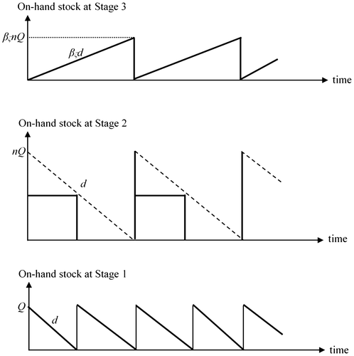
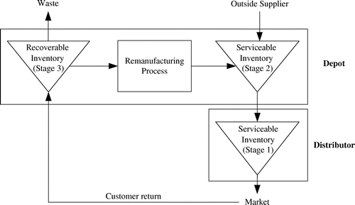
There are three stages of inventory considered in the model, i.e. Stage 1, Stage 2, and Stage 3. As shown in Figure 1, Stage 1 refers to the serviceable inventory kept by the distributor, Stage 2 refers to the serviceable inventory stored by the depot, and Stage 3 refers to the recoverable used item inventory at the depot. Depot delivers finished good items to distributor in n shipments, where each shipment contains Q units of product. It is assumed that the orders received from outside suppliers and finished goods produced from the remanufacturing process will arrive simultaneously at the beginning of each cycle in Stage 2. Where the lead time delivery from Stage 1 to Stage 2 is assumed to be zero.

Figure 1. A single depot-single distributor inventory system with returns (Mitra, 2009).

Each unit of items will go through several remanufacturing generations before it has to be disposed as a waste. The number of generations itself is depended upon the annual investment costs paid by the depot. The higher the number of remanufacturing generations, the greater the costs need to be paid by the depot in term of remanufacturing investment. In this model, we also consider some costs associated with environmental implications, i.e. carbon emission cost and energy cost. Carbon emissions cost measured by Green-House-Gas (GHG) emissions is incurred for each transportation activity and remanufacturing process performed by the depot and the distributor. While energy cost is measured by the consumption of energy (kWh) spent on each remanufacturing process. Land transportation is assumed, where items in the serviceable inventory are delivered from the depot to the distributor by trucks and are then returned to the depot after the used items has been collected by the distributor from the market. The system cost parameters considered in the model are listed as follows:

(1)	Holding costs at Stage 1, 2, and 3.
(2)	Set-up costs at Stage 1, 2, and 3.
(3)	Cost for remanufacturing.
(4)	Cost for purchasing from outside suppliers.
(5)	Annual investment cost.
(6)	Waste disposal cost.
(7)	Finished goods and return items transportation cost.
(8)	GHG emissions cost from transportation.
(9)	GHG emissions cost from remanufacturing.
(10)	Energy consumption cost for remanufacturing.

In this study, we intend to obtain minimum annual joint inventory cost function (AJTC) by determining the following decision variables:

n	=	number of shipments from Stage 2 to Stage 1, w.r.t n ≥ 1 and an integer
Q	=	shipment lot size from Stage 2 to Stage 1 (unit)
ζ	=	number of remanufacturing generations, w.r.t ζ ≥  0 and an integer

The parameters used in this model following with their notations and constraints are listed as follows:

β	=	nominal proportion of items returned for remanufacturing when an item is remanufactured for an unlimited number of times (ζ = ∞), where 0 ≤ β < 1
βζ	=	actual proportion of items returned for remanufacturing when an item is recovered for a limited ζ number of times (ζ ≥ 0), where βζ = $1-\left[\frac{(1-\mathit{\beta })}{(1-{\mathit{\beta }}^{\mathit{\zeta }+1})}\right]$
hi	=	holding cost per unit per unit of time at Stage i ($/unit/year), where i = 1, 2, 3
Ai	=	set-up cost at Stage i ($), where i = 1, 2, 3
d	=	annual demand rate (units/year)
cinv	=	annual investment in the design process of the product to, theoretically, be able to remanufacture it for an indefinite number of times ($/year)
θ	=	investment increment factor that governs the ratio of investment for each remanufactured generation, where 0 ≤ θ < 1
v	=	annual remanufacturing rate (units/year), where v > d
Ft	=	fixed cost per truck per trip ($/truck)
tc	=	truck capacity (units/truck)
gt	=	number of gallons per truck per distance travelled (gallons/truck)
et	=	amount of GHG emissions from one gallon of diesel-truck fuel (ton/gallon)
cec	=	carbon emissions tax per ton of GHG emissions ($/ton)
ar	=	emissions function parameter for remanufacturing (ton year2/unit3)
br	=	emissions function parameter for remanufacturing (ton year/unit2)
cr	=	emissions function parameter for remanufacturing (ton/unit)
C′0	=	the required energy at the machine to remanufacture one unit (kWh/unit)
C′1	=	the required energy per year when remanufacturing is idle (kWh/year)
Cen	=	cost of energy ($/kWh)
Ps	=	purchasing price from outside supplier ($/unit)
Cr	=	remanufacturing cost per unit ($/unit)
Cw	=	disposal cost per unit ($/unit)

Here are the assumptions used in the model.

(1)	Demand (d) is known at a constant rate (deterministic).
(2)	Lead time for transportation and remanufacture equals to zero.
(3)	Remanufacturing rate is always greater than demand rate (v > d).
(4)	Return rate is always less than demand rate (r < d).
(5)	Remanufactured items have the same quality level as the new items (as-good-as-new-one).
(6)	There are no defective items (perfect remanufacturing process).
(7)	Warehouse capacity is unlimited.
(8)	Orders received from outside suppliers and finished goods produced from the recovery process will arrive simultaneously at the beginning of each cycle in Stage 2.

3.1. Cost functions

Figure 2 shows the on-hand inventory levels at Stage 1, 2, and 3 with n = 2. From Figure 2, the average echelon inventories at Stage 1, 2, and 3 can be known as Q/2, nQ/2, and $\frac{nQ}{2}\left(1-\frac{1-\mathit{\beta }}{1-{\mathit{\beta }}^{1+\mathit{\zeta }}}\right)$ units, respectively. Then, the annual holding cost (C_H) for Stage 1 (C_H1), Stage 2 (C_H2), and Stage 3 (C_H3) can be calculated as follows:(1) $$C_{\text{H}}=\frac{1}{2}\left(h_1-h_2\right)Q+\frac{h_{2}nQ}{2}+\frac{1}{2}{h}_{3}nQ\left(1-\frac{1-\mathit{\beta }}{1-{\mathit{\beta }}^{1+\mathit{\zeta }}}\right)$$(1)

Figure 2. Inventory level for Stage 1, 2, and 3 over time (n = 2).

The number of setups per unit time at Stage 1, Stage 2, and Stage 3 are d/Q, d/(nQ), and d/(nQ), respectively. Apparently, the annual setup cost (C_S) for Stage 1 (C_S1), Stage 2 (C_S2), and Stage 3 (C_S3) can be expressed as follows:(2) $$C_{\text{S}}=\frac{A_{1}d}{Q}+\frac{A_{2}d}{nQ}+\frac{A_{3}d\left(1-\frac{1-\mathit{\beta }}{1-{\mathit{\beta }}^{1+\mathit{\zeta }}}\right)}{nQ}$$(2)

The annual cost to remanufacture (C_R) is a remanufacturing cost for all recovered used items per year, which is given by(3) $$C_{\text{R}}=C_{\text{r}}d\left(1-\frac{1-\mathit{\beta }}{1-{\mathit{\beta }}^{1+\mathit{\zeta }}}\right)$$(3)

The annual purchasing cost from outside supplier (C_os) is purchasing cost for the rest of the annual demand that cannot be met from recovered items, which is expressed as follows:(3) $$C_{\text{os}}=P_{\text{S}}d\left(1-\frac{1-\mathit{\beta }}{1-{\mathit{\beta }}^{1+\mathit{\zeta }}}\right)$$(3)

The annual investment cost (C_inv) is investment costs related to the design process that incurred per year and paid by the vendor to be able to remanufacture its used items at a limited number of times. The function of C_inv is taken from El Saadany et al. (2013) and is given by(4) $$C_{\text{inv}}=c_{\text{inv}}(1-e^{-\mathit{\zeta }\mathit{\theta }})$$(4)

The annual waste disposal cost (C_w) is costs incurred by the vendor to dispose used items that cannot be remanufactured any longer. The function of C_w is given by(5) $$C_{\text{w}}=c_{\text{w}}d\left(1-\frac{1-\mathit{\beta }}{1-{\mathit{\beta }}^{1+\mathit{\zeta }}}\right)$$(5)

The transportation cost (C_t) consists of costs incurred by the depot and distributors related to transportation activities for items purchased from outside suppliers, finished items shipped to distributor, as well as the return items collected from the market, which can be calculated by the following equation:(6) $$C_{\text{t}}=\frac{d{F}_{\text{t}}}{t_{\text{C}}}+\frac{d{F}_{\text{t}}(1-{\mathit{\beta }}_{\mathit{\zeta }}+{\mathit{\beta }}_{\mathit{\zeta }})}{t_{\text{C}}}+\frac{d{F}_{\text{t}}(1-{\mathit{\beta }}_{\mathit{\zeta }})}{t_{\text{C}}}=\frac{2d{F}_{\text{t}}}{t_{\text{C}}}+\frac{d{F}_{\text{t}}(1-\mathit{\beta })}{t_{\text{C}}(1-{\mathit{\beta }}^{1+\mathit{\zeta }})}$$(6)

As explained in Bazan et al. (2015), the relationship for GHG emissions is taken from Bogaschewsky (1995) which has already been validated empirically in Narita (2012). The function of GHG emission cost (C_GHGe) is used for remanufacturing process and can be calculated by(7) $$C_{\text{GHGe}}=c_{\text{ec}}d(c_{\text{r}}-b_{\text{r}}v+a_{\text{r}}{v}^2)\left(1-\frac{1-\mathit{\beta }}{1-{\mathit{\beta }}^{1+\mathit{\zeta }}}\right)$$(7)

The annual GHG emission cost related to transportation activity is given in term of the amount GHG emissions emitted from using a gallon of fuel. The function of C_GHGt can be estimated by the following equation(8) $$C_{\text{GHGt}}=g_{\text{t}}{e}_{\text{t}}{e}_{\text{c}}\left(\frac{d}{t_{\text{C}}}+\frac{d(1-{\mathit{\beta }}_{\mathit{\zeta }}+{\mathit{\beta }}_{\mathit{\zeta }})}{t_{\text{C}}}+\frac{d(1-{\mathit{\beta }}_{\mathit{\zeta }})}{t_{\text{C}}}\right)=g_{\text{t}}{e}_{\text{t}}{e}_{\text{c}}\left(\frac{2d}{t_{\text{C}}}+\frac{d(1-\mathit{\beta })}{t_{\text{C}}(1-{\mathit{\beta }}^{1+\mathit{\zeta }})}\right)$$(8)

Since there is only one manufacturing process which is remanufacturing, the energy consumption appears on the remanufacturing process only. The cost of energy per year (C_N) can be expressed below(9) $$C_{\text{N}}=C_{\text{en}}d\left(C^{\prime }0+\frac{C^{\prime }1}{v}\right)\left(1-\frac{1-\mathit{\beta }}{1-{\mathit{\beta }}^{1+\mathit{\zeta }}}\right)$$(9)

Hence, the annual joint inventory cost (AJTC) for both parties is a sum of the above mentioned costs and can be written as follows:$$\text{AJTC}(n,Q,\mathit{\zeta })=\frac{A_{1}d}{Q}+\frac{A_{2}d}{nQ}+\frac{A_{3}d}{nQ}+\frac{1}{2}\left(h_1-h_2\right)Q+\frac{h_{2}nQ}{2}+\frac{1}{2}{h}_{3}nQ\left(1-\frac{1-\mathit{\beta }}{1-{\mathit{\beta }}^{1+\mathit{\zeta }}}\right)+C_{\text{r}}d\left(1-\frac{1-\mathit{\beta }}{1-{\mathit{\beta }}^{1+\mathit{\zeta }}}\right)+$$$$P_{\text{S}}d\left(1-\frac{1-\mathit{\beta }}{1-{\mathit{\beta }}^{1+\mathit{\zeta }}}\right)+c_{\text{inv}}\left(1-e^{-\mathit{\zeta }\mathit{\theta }}\right)+c_{\text{w}}d\left(1-\frac{1-\mathit{\beta }}{1-{\mathit{\beta }}^{1+\mathit{\zeta }}}\right)+\frac{2d{F}_{\text{t}}}{t_{\text{C}}}+\frac{d{F}_{\text{t}}(1-\mathit{\beta })}{t_{\text{C}}(1-{\mathit{\beta }}^{1+\mathit{\zeta }})}+$$(10) $$c_{\text{ec}}d(c_{\text{r}}-b_{\text{r}}v+a_{\text{r}}{v}^2)\left(1-\frac{1-\mathit{\beta }}{1-{\mathit{\beta }}^{1+\mathit{\zeta }}}\right)+g_{\text{t}}{e}_{\text{t}}{e}_{\text{c}}\left(\frac{2d}{t_{\text{C}}}+\frac{d(1-\mathit{\beta })}{t_{\text{C}}(1-{\mathit{\beta }}^{1+\mathit{\zeta }})}\right)+C_{\text{en}}d\left(C^{\prime }0+\frac{C^{\prime }1}{v}\right)\left(1-\frac{1-\mathit{\beta }}{1-{\mathit{\beta }}^{1+\mathit{\zeta }}}\right)$$(10)

3.2. Solution procedure

The optimization problem is to determine the values of n, Q, and ζ that minimize AJTC (n, Q, ζ). The optimal solutions of Q are found by taking the first partial derivative of Equation (10) with respect to Q, and then setting the result to zero. The optimal values of Q denoted by Q^* are derived as follows:(11) $$\frac{\text{dAJTC}(n,Q,\mathit{\zeta })}{\text{d}Q}=\frac{h_1-h_2}{2}+\frac{h_{2}n}{2}-\frac{A_{1}d}{Q^2}-\frac{A_{2}d}{n{Q}^2}-\frac{A_{3}d}{n{Q}^2}+\frac{1}{2}{h}_{3}n\left(1-\frac{1-\mathit{\beta }}{1-{\mathit{\beta }}^{1+\mathit{\zeta }}}\right)=0$$(11) (12) $$Q^{\ast }(n,\mathit{\zeta })=\sqrt{\frac{2d(A_3\mathit{\beta }(-1+{\mathit{\beta }}^{\mathit{\zeta }})+A_2(-1+{\mathit{\beta }}^{1+\mathit{\zeta }})+A_{1}n(-1+{\mathit{\beta }}^{1+\mathit{\zeta }}))}{n(h_{3}n\mathit{\beta }(-1+{\mathit{\beta }}^{\mathit{\zeta }})+h_1(-1+{\mathit{\beta }}^{1+\mathit{\zeta }})+h_2(-1+n)(-1+{\mathit{\beta }}^{1+\mathit{\zeta }}))}}$$(12)

The optimal value of n denoted by n^* can be obtained by letting the derivative of Equation (10) with respect to n equal to zero and then substituting the value of Q^* in Equation (12). We obtain the following function(13) $$n^{\ast }=\sqrt{\frac{(-h_1+h_2)(A_3\mathit{\beta }(-1+{\mathit{\beta }}^{\mathit{\zeta }})+A_2(-1+{\mathit{\beta }}^{1+\mathit{\zeta }}))}{-A_1(h_3\mathit{\beta }(-1+{\mathit{\beta }}^{\mathit{\zeta }})+h_2(-1+{\mathit{\beta }}^{1+\mathit{\zeta }}))}}$$(13)

The convexity of the cost function, AJTC, with respect to the decision variables, Q and n, is proven by the Hessian matrix that must be positive definite. Hence, these following conditions should be satisfied:(14) $$\frac{{\text{d}}^{″}\text{AJTC}}{\text{d}{Q}^{″}}=\frac{2A_{1}d}{Q^3}+\frac{2A_{2}d}{n{Q}^3}+\frac{2A_{3}d\left(1-\frac{1-\mathit{\beta }}{1-{\mathit{\beta }}^{1+\mathit{\zeta }}}\right)}{n{Q}^3}>0$$(14) (15) $$\frac{{\text{d}}^{″}\text{AJTC}}{\text{d}{n}^{″}}=\frac{2A_{2}d}{n^{3}Q}+\frac{2A_{3}d(1-\frac{1-\mathit{\beta }}{1-{\mathit{\beta }}^{1+\mathit{\zeta }}})}{n^{3}Q}>0$$(15) $$\left[\frac{{\text{d}}^{″}\text{AJTC}}{\text{d}{Q}^{″}}\right]\left[\frac{{\text{d}}^{″}\text{AJTC}}{\text{d}{n}^{″}}\right]-\left[\frac{{\text{d}}^{″}\text{AJTC}}{\text{d}Q\text{d}n}\right]\left[\frac{{\text{d}}^{″}\text{AJTC}}{\text{d}n\text{d}Q}\right]>0$$$$=\left(\frac{2A_{1}d}{Q^3}+\frac{2A_{2}d}{n{Q}^3}+\frac{2A_{3}d\left(1-\frac{1-\mathit{\beta }}{1-{\mathit{\beta }}^{1+\mathit{\zeta }}}\right)}{n{Q}^3}\right)\left(\frac{2A_{2}d}{n^{3}Q}+\frac{2A_{3}d\left(1-\frac{1-\mathit{\beta }}{1-{\mathit{\beta }}^{1+\mathit{\zeta }}}\right)}{n^{3}Q}\right)>$$(16) $${\left(\frac{h_2}{2}+\frac{A_{2}d}{n^2{Q}^2}+\frac{1}{2}{h}_3\left(1-\frac{1-\mathit{\beta }}{1-{\mathit{\beta }}^{1+\mathit{\zeta }}}\right)+\frac{A_{3}d\left(1-\frac{1-\mathit{\beta }}{1-{\mathit{\beta }}^{1+\mathit{\zeta }}}\right)}{n^2{Q}^2}\right)}^2$$(16)

In Equation (16), as the value of the left-hand side is always greater than the right-hand side, the above condition is satisfied. Therefore, as those three conditions are satisfied, AJTC is proven to be convex with respect to Q and n. The optimal value of n, Q, and ζ that minimize AJTC (n, Q, ζ) for the value of 1 ≤ ζ ≤ 10 is derived by the following solution procedure.

• Step 1 For each value of ζ for 1 ≤ ζ ≤ 10, calculate the value of n and Q using Equations (12) and (13), respectively. If n is not an integer, then set n = n and n = n then continue to step 2.

• Step 2 Calculate the value of AJTC (n, Q, ζ) for n = n and n = n.

• Step 3 Find the combination value of n, Q, and ζ that gives the minimum value of AJTC (n, Q, ζ), and set as n^*, Q^*, and ζ^*.

4. Numerical example

To illustrate the model that has been developed in this study, we provide a numerical example and solve the problem by using the proposed solution procedure explained in the previous section. As we use the model belongs to Mitra (2009) and the model belongs to Bazan et al. (2015) as our basic models, hence we also adopt the numerical value for each parameter from those studies. Bazan et al. (2015) stated that the system of remanufacturing is suitable for many kinds of products, such as: retreaded tires, heavy-duty and off-road (HDOR) equipment, motor vehicle parts, consumer products, IT products, wholesalers, machinery, aerospace, and medical devices. The parameters used to illustrate the problem are: β = 0.67, h₁ = 5 $/unit/year, h₂ = 3 $/unit/year, h₃ = 1.5 $/unit/year, d = 100 units/year, A₁ = 50 $/batch, A₂ = 200 $/batch, A₃ = 100 $/batch, c_inv = 500 $/year, θ = 0.2, v = 150 units/year, F_t = 15 $/truck, t_c = 50 units/truck, g_t = 375 gallons/truck, e_t = 0.01008414 tons/gallon, c_ec = 1 $/ton, a_r = 0.000000000833 ton years²/unit³, b_r = 0.0002 ton years/unit², c_r = 1.4 tons/unit, C′0 = 0.189 KWh/unit, C′1 = 6051.10 KWh/year, C_en = 0.00928 $/KWh, P_s = 20 $/unit, C_r = 10 $/unit, c_w = 3 $/unit.

By applying the solution procedure given in the Section 3.2, we generate the results that minimize the value of AJTC. From Table 1, the optimal solution for each decision variable of the proposed model can easily be found by comparing the value of AJTC. The optimal value of n is 1.6329, since n has to be an integer, we take approximation values of n^* as n^* and n^* which are 1 and 2.

As shown in Table 2, it is clearly seen that the optimal solution of the model is obtained when the number of shipments from the depot to the distributor (n^*) is 2 shipments with quantity per shipment (Q^*) is 60 units, and the remanufacturing generation (ζ^*) is 2 generations. Those optimal values of n^*, Q^*, and ζ^* give the minimum value of AJTC that is $2,560.71.

Table 2. The optimization results for the proposed model (1 ≤ ζ ≤ 10)

ζ	βζ	n*	Q*	Depot inventory cost	Distributor inventory cost	AJTC
1	0.401198	2	59.51	$2,442.28	$166.02	$2,608.31
2*	0.528057*	2*	59.07	$2,399.27	$161.44	$2,560.71
3	0.586719	2	58.88	$2,405.82	$159.32	$2,565.15
4	0.618492	2	58.78	$2,426.21	$158.18	$2,584.38
5	0.63718	2	58.72	$2,449.66	$157.50	$2,607.16
6	0.648709	2	58.68	$2,472.35	$157.08	$2,629.43
7	0.656033	2	58.66	$2,492.88	$156.82	$2,649.69
8	0.660771	2	58.65	$2,510.85	$156.65	$2,667.49
9	0.663873	2	58.64	$2,526.23	$156.58	$2,682.81
10	0.66592	2	58.63	$2,539.37	$156.46	$2,695.83

* Optimal solution for the proposed model

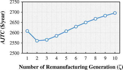
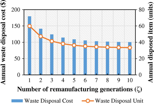
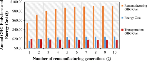
From the results, we can point out some important notes, including the effect of remanufacturing generations (ζ) on AJTC, annual waste disposal cost (C_w), annual GHG emission cost (C_GHGt and C_GHGe) and also on annual energy cost (C_N) which are represented in Figures 3^{Figure 4}–5, respectively.

Figure 3. The effect of ζ on AJTC.

Figure 4. The effects of ζ on C_w and annual disposed items.

Figure 5. The effects of ζ on C_GHGe, C_GHGt, and C_N.

Figure 3 shows the effect of ζ on annual joint inventory cost (AJTC). The interesting point is, AJTC can be minimized when the value of ζ is 2, which decreases the value of AJTC by $47.59. Meanwhile, when the value of ζ is increased to 3, there is an increasing value on AJTC as well as if the value of ζ is increased to 4, 5, and so on. It proves that ζ gives convex effects on AJTC, hence the optimal value of ζ should be determined to obtain the minimum inventory cost.

Another point should be taken into considerations is the environmental effect that may be generated by the system, including annual disposed items, annual CO₂ released, and annual kWh usage. As shown in Figure 4, the amount of disposed items per year decreases while the number of remanufacturing generations increases. It indicates that if an item is more remanufacturable, then it will be more environmentally sustainable since the amount of disposed items is lower. However, if we take the amount of CO₂ released and the amount of kWh usage per year as our focus, related to the environmental consideration, we can point out that more remanufacturing generations will end up to more GHG emissions and energy cost.

From Figure 5, it can be seen that increasing ζ gives increasing GHG emissions cost related to the remanufacturing process (C_GHGe) and energy cost (C_N) and decreasing the GHG emission cost related to transportation (C_GHGt). Apparently, it is because the depot only performs remanufacturing process. The depot fulfils the distributor demand by running remanufacturing process and the rest of the demand is met by orders items from outside supplier. The depot does not perform any other process, such as a manufacturing process. Therefore, GHG emissions and energy consumption related to manufacturing operations are not generated. Consequently, higher number of remanufacturing generations does not reduce but rather increase the cost related to GHG emissions and energy consumption. An increase in GHG emission related to remanufacturing process and transportation is not followed by a decrease in energy released and usage by other processes, such as a manufacturing process.

5. Sensitivity analysis

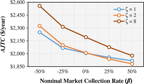
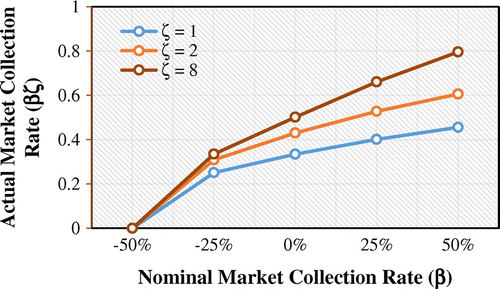
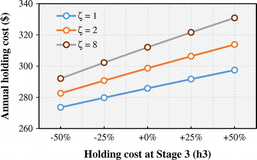
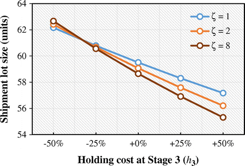
The sensitivity analysis was conducted to observe the behaviour of the model in dealing with uncertainty of the exact values of some uncontrollable parameters in real system. The sensitivity analysis is done by observing the value of AJTC when β, h₃, and C_inv are changed. The results of the sensitivity analysis are shown in Figures 6–10.

Figure 6. The effects of β on AJTC.

Figure 7. The effects of β on β_ζ.

Figure 8. The effects of h₃ on annual holding cost.

Figure 9. The effects of h₃ on optimal shipping lot size (Q^*).

Figure 10. The effects of c_inv on AJTC.

By changing the value of β, the value of AJTC will change as well. As explained in the previous section, β is a nominal proportion of used items for remanufacturing when an item is remanufactured for an unlimited number of times (ζ = ∞). While β_ζ is the actual proportion of used items for remanufacturing when an item is remanufactured for a limited number of times. The difference between β and β_ζ itself has been defined by El Saadany et al. (2013). From Figure 7, it is known that increases in β will affect the value of β_ζ to be higher which means the amount of items for remanufacturing is greater. Figure 6 shows that higher value of β will lower the value of AJTC. In other words, the more items can be remanufactured, the lower annual inventory cost would be. This suggests that remanufacturing process is more economical compared to order from outside suppliers. In addition, the remanufacturing process is also more environmentally friendly. By performing the process, the amount of waste on the market can be reduced.

The changes in the value of h₃ will affect AJTC through annual holding cost. As explained in the previous section, h₃ stands for inventory holding cost per unit for Stage 3, which is recoverable item inventory at the depot. From Figure 8, it is known that an increase in the value of h₃ provides higher annual holding cost. However, the increases are not significant. By increasing the value of h₃ by 50%, the holding cost only increases by 4%. This is because the changes in the value of h₃ also followed by a change in the optimal value of shipping lot size (Q^*) as shown in Figure 9. To minimize the losses, when the holding cost is higher, the model will adjust the inventory system by reducing the optimal shipping lot size. It can be concluded that if the holding cost is rising, then the lot size will be decreased by the model in order to minimize total cost.

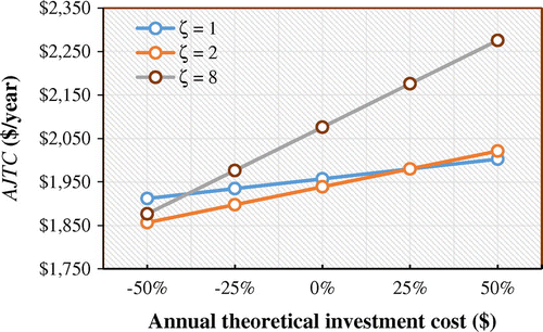
In real case, there is actually an uncertainty in term of “how much should we spend on investment if we desire a certain number of remanufacturing generation?”, since we could not estimate the exact amount on investment cost has to be spent on the system. Therefore, we should conduct an analysis regarding the effects of c_inv on AJTC to be able to construct a proper planning. As we already know, c_inv represents the annual investment in the design process of the product to, theoretically, be able to remanufacture it for an indefinite number of times. Figure 10 shows the effects of c_inv on AJTC.

It is observed that higher c_inv will end up in the increasing value of AJTC. For higher value of ζ, the margin generated is increased rapidly. This also led to a shift in the optimal value of ζ. Increasing c_inv by 25% actually give a change on ζ^*, from 2 to 1 generation only. It implies that in case of high annual investment cost, the management should not spend too much on investment only to gain higher remanufacturing generation. On the contrary, lower remanufacturing generation actually gives a worse effect to the environment.

6. Conclusions

This study investigates issues in the reversed supply chain by considering an integrated inventory decision-making and also examines the environmental effects that may be generated by the system. Previous works on this problem only consider a single-echelon problem and indefinite number of remanufacturing without taking limited remanufacturing and integrated inventory decision-making among parties in the supply chain into consideration. In this paper, we develop an inventory model consisting a depot and a distributor while the depot performs remanufacturing process to recover returned items collected from the market. We also consider a limited number of times that an item can be remanufactured since in some cases items cannot be remanufactured or repaired at indefinite number of times. Moreover, this model also includes the environmental effect by incorporating some costs, including GHG emissions cost and energy cost.

The results from the study show that the number of remanufacturing generations gives significant impact on disposal cost. If the number of remanufacturing generations increases, the number of disposed items increases as well. Thus, if an item is more remanufacturable, then it will be more environmentally sustainable. The larger the number of remanufacturing generations, the larger GHG emissions and energy cost. When there is more number of shipments in the system, the depot tends to decrease the amount of items per shipment so that the holding cost can be reduced. The increase of holding cost at Stage 3 will eventually decrease the optimal value of shipment lot size. Yet, the number of shipments was not influenced by changes in related parameters. The results also show that the optimal number of remanufacturing generations tends to be higher where the investment cost related to product design is lower. From the sensitivity results, it is known that where the investment cost is increasing by 25%, the optimal number of remanufacturing generations was shifted from 2 to 1 generation only.

As the demand and returns in this model are assumed to be deterministic at a constant rate, we suggest that this model can be applied to real system for such company or supply chain with a small variation of the demand and returns. For a system that actually has a high variation of demand and returns, this model can still be implemented by considering safety stock of serviceable product at the distributor and safety stock of used product at the depot.

There are some issues that should be taken into consideration for future modelling. The first one is interactions between demand processes for new and remanufactured products. Some products, especially remanufacturable technology product, are actually do not meet the perfect substitution assumption. The current researches have not accommodated more complex practical settings. Secondly, it is the interactions between multiple items. The existing literatures mainly analyze a single-item problem, without considering a system that consists of multi-item with interactions that may be presented among different types of items. The third one is interactions between demand and returns. This study assumes the demand and return rate to be independent. In real case, the correlation between demand and return rate is actually well known. For future research, the model can be developed by including correlated demand and returns. Another thing which is not less important is modelling the uncertainties in term of time, quantity, quality of used items and another things that also included in product acquisition. Lechner and Reimann (2014), emphasize that uncertainties in product acquisition affect both manufacturing and remanufacturing strategies. The return rate is possible to be controlled if the company spent a specific acquisition effort. The thing becomes more challenging since it directly influences remanufacturing quantity, cost, and also lead-time in a more complex way.

Funding

The authors received no direct funding for this research.

Additional information

Notes on contributors

Anindya Rachma Dwicahyani

Anindya Rachma Dwicahyani is a Senior researcher in Production System Laboratory, Sebelas Maret University. Her research interests are inventory management, production management and operations research.

Wakhid Ahmad Jauhari

Wakhid Ahmad Jauhari is currently a Lecturer in Sebelas Maret University. He obtained Bachelor and Master degrees, both in Industrial Engineering, from Sepuluh Nopember Institute of Technology (ITS) in Surabaya, Indonesia. His research interests include modelling inventory, supply chain management and manufacturing design.

Cucuk Nur Rosyidi

Cucuk Nur Rosyidi is a Lecturer in Industrial Engineering Department of Sebelas Maret University. His doctoral degree was obtained from Institut Teknologi Bandung Indonesia in the field of Manufacturing Systems in 2010. His research interests include product design and development, quality engineering, and system modeling.

Pringgo Widyo Laksono

Pringgo Widyo Laksono is a Lecturer in Industrial Engineering Department of Sebelas Maret University. His master degree was obtained from Universitas Gadjah Mada in the field of Industrial Engineering in 2012. His research interests include industrial engineering science such as production and manufacturing systems, design working system, optimisation, and operation management.

References

- Agrawal, S., Singh, R. K., & Murtaza, Q. (2015). A literature review and perspectives in reverse logistics. Resources, Conservation and Recycling, 97, 76–92.10.1016/j.resconrec.2015.02.009
- Bazan, E., Jaber, M. Y., & El Saadany, A. M. A. (2015). Carbon emissions and energy effects on manufacturing–remanufacturing inventory models. Computers and Industrial Engineering, 88, 307–316.10.1016/j.cie.2015.07.002
- Bazan, E., Jaber, M. Y., & Zanoni, S. (2016). A review of mathematical inventory models for reverse logistics and the future of its modeling: An environmental perspective. Applied Mathematical Modelling, 40, 4151–4178.10.1016/j.apm.2015.11.027
- Bazan, E., Jaber, M. Y., & Zanoni, S. (2017). Carbon emissions and energy effects on a two-level manufacturer-retailer closed-loop supply chain model with remanufacturing subject to different coordination mechanisms. International Journal of Production Economics, 183, 394–408.
- Bagaschewsky, R. (1995). Natürliche Umwelt und Produktion. Wiesbaden: Gabler-Verlag.
- Bei, W., & Linyan, S. (2005). A review of reverse logistics. Applied Sciences, 7, 16–29.
- Bonney, M., & Jaber, M. Y. (2011). Environmentally responsible inventory models: Non-classical models for a non-classical era. International Journal of Production Economics, 133, 43–53.10.1016/j.ijpe.2009.10.033
- Cobb, B. R. (2016). Inventory control for returnable transport items in a closed-loop supply chain. Transportation Research Part E: Logistics and Transportation Review, 86, 53–68.10.1016/j.tre.2015.12.010
- Chung, S. L., & Wee, H. M. (2008). Green-component life-cycle value on design and reverse manufacturing in semi-closed supply chain. International Journal of Production Economics, 113, 528–545.10.1016/j.ijpe.2007.10.020
- Chung, S. L., Wee, H. M., & Yang, P. C. (2008). Optimal policy for a closed-loop supply chain inventory system with remanufacturing. Mathematical and Computer Modelling, 48, 867–881.10.1016/j.mcm.2007.11.014
- El Saadany, A. M. A., Jaber, M. Y., & Bonney, M. (2013). How many times to remanufacture? International Journal of Production Economics, 143, 598–604.10.1016/j.ijpe.2011.11.017
- Ferrer, G. (1997). The economics of tire remanufacturing. Resources, Conservation and Recycling, 19, 221–255.10.1016/S0921-3449(96)01181-0
- Fleischmann, M., Bloemhof-Ruwaard, J. M., Dekker, R., van der Laan, E., van Nunen, J. A. E. E., & Van Wassenhove, L. N. (1997). Quantitative models for reverse logistics: A review. European Journal of Operational Research, 103, 1–17.10.1016/S0377-2217(97)00230-0
- Giri, B. C., & Sharma, S. (2015). Optimizing a closed-loop supply chain with manufacturing defects and quality dependent return rate. Journal of Manufacturing Systems, 35, 92–111.10.1016/j.jmsy.2014.11.014
- Gu, Q., & Tagaras, G. (2014). Optimal collection and remanufacturing decisions in reverse supply chains with collector’s imperfect sorting. International Journal of Production Research, 52, 5155–5170.10.1080/00207543.2014.899720
- Guide, V. D. R., & Van Wassenhove, L. N. V. (2009). The evolution of closed-loop supply chain research. Operations Research, 57, 10–18.10.1287/opre.1080.0628
- Heese, H. S., Cattani, K., Ferrer, G., Gilland, W., & Roth, A. V. (2005). Competitive advantage through take-back of used products. European Journal of Operational Research, 164, 143–157.10.1016/j.ejor.2003.11.008
- Jaber, M. Y., Zanoni, S., & Zavanella, L. E. (2014). A consignment stock coordination scheme for the production, remanufacturing, and waste disposal problem. International Journal of Production Research, 52, 50–65.10.1080/00207543.2013.827804
- Jauhari, W. A., Dwicahyani, A. R., & Kurdhi, N. A. (2017). Lot sizing decisions in a closed-loop supply chain system with remanufacturing. International Journal of Procurement Management, 10, 381–409.10.1504/IJPM.2017.083469
- Jauhari, W. A., Mayangsari, S., Kurdhi, N. A., & Wong, K. Y. (2017). A fuzzy periodic review integrated inventory model involving stochastic demand, imperfect production process and inspection errors. Cogent Engineering, 2017(4), 1308653.
- Jauhari, W. A., Pamuji, A. S., & Rosyidi, C. N. (2014). Cooperative inventory model for vendor-buyer system with unequal-sized shipment, defective items and carbon emission cost. International Journal of Logistics Systems and Management, 19, 163–186.10.1504/IJLSM.2014.064657
- Lechner, G., & Reimann, M. (2014). Impact of product acquisition on manufacturing and remanufacturing strategies. Production & Manufacturing Research, 2, 831–859.10.1080/21693277.2014.976881
- Mabini, M. C., Pintelon, L. M., & Gelders, L. F. (1992). EOQ type formulations for controlling repairable inventories. International Journal of Production Economics, 28, 21–33.10.1016/0925-5273(92)90110-S
- Minner, S. (2001). Strategic safety stocks in reverse logistics supply chains. International Journal of Production Economics, 71, 417–428.10.1016/S0925-5273(00)00138-9
- Mitra, S. (2009). Analysis of a two-Chelon inventory system with returns. International Journal of Management Science, 37, 106–115.
- Mitra, S. (2012). Inventory management in a two-echelon closed-loop supply chain with correlated demands and returns. Computers & Industrial Engineering, 62, 870–879.10.1016/j.cie.2011.12.008
- Mohanty, R. P., & Prakash, A. (2014). Green supply chain management practices in India: An empirical study. Production Planning & Control, 25, 1322–1337.10.1080/09537287.2013.832822
- Nahmias, N., & Rivera, H. (1979). A deterministic model for a repairable item inventory system with a finite repair rate†. International Journal of Production Research, 17, 215–221.10.1080/00207547908919609
- Narita, H. (2012). Environmental burden analyzer for machine tool operations and its application. In Faieza Abdul Aziz (Ed.), Manufacturing system. Rijeka: InTech Europe. Retrieved from http://cdn.intechopen.com/pdfs-wm/36413.pdf
- Radzuan, K., Othman, A. A., Anuar, H. S., & Osman, W. N. (2014). Measuring the impact of inventory control practices: A conceptual framework. In 4th International Conference on Technology and Operations Management.
- Richter, K. (1996a). The EOQ repair and waste disposal model with variable setup numbers. European Journal of Operational Research, 95, 313–324.10.1016/0377-2217(95)00276-6
- Richter, K. (1996b). The extended EOQ repair and waste disposal model. International Journal of Production Economics, 45, 443–447.10.1016/0925-5273(95)00143-3
- Richter, K. (1997). Pure and mixed strategies for the EOQ repair and waste disposal problem. OR Spektrum, 19, 123–129.10.1007/BF01545511
- Russel, R. S., & Taylor, B. W. (2006). Operations management (5th ed.). Boston, MA: Prentice-Hall.
- Sasikumar, P., & Kannan, G. (2008). Issues in reverse supply chains, part I: End-of-life product recovery and inventory management–an overview. International Journal of Sustainable Engineering, 1, 154–172.10.1080/19397030802433860
- Sasikumar, P., & Kannan, G. (2009). Issues in reverse supply chain, part III: Classification and simple analysis. International Journal of Sustainable Engineering, 2, 2–27.10.1080/19397030802673374
- Shcrady, D. A. (1967). A deterministic inventory model for repairable items. Naval Research Logistics Quarterly, 14, 391–398.
- Srivastava, S. K. (2007). Green supply-chain management: A state-of-the-art literature review. International Journal of Management Reviews, 9, 53–80.10.1111/ijmr.2007.9.issue-1
- Xia, W. H., Jia, D. Y., & He, Y. Y. (2011). The remanufacturing reverse logistics management based on closed-loop supply chain management processes. Procedia Environmental Sciences, 11, 351–354.
- Yogi, K. S. (2015). Performance evaluation of reverse logistics: A case of LPG agency. Cogent Business & Management, 2015(2), 1063229.
- Yuan, K. F., & Gao, Y. (2010). Inventory decision-making models for a closed-loop supply chain system. International Journal of Production Research, 48, 6155–6187.10.1080/00207540903173637