Optimization of the fleet per shovel productivity in surface mining: Case study of Chilanga Cement, Lusaka Zambia

Abstract

A well-organized fleet management in surface mining is required in order to maximize truck per shovel Match Factors. The most common materials handling in surface mining is by truck and shovel combination. This operation is one of the key factor to reduce the cost of mineral production. This paper presents a complete methodology that can be used to determine the number of trucks required per shovel during striping and the extraction of minerals for Surface mining. The methodology is based on the reduction of the queuing time of the trucks at the loading point. The visual studio was used to develop applications based on DOT.NET platform and some of the basic programming pseudocode are highlighted in this context. This application is quick and easy to understand and will help fasten the calculation of open pit parameters as discussed in the paper as well as a match factor of 1.07 was calculated.

Keywords:

• bulk density
• fill factor
• match factor
• queuing length

Public Interest Statement

The most common transportation and loading equipments in surface mining is via the combination of truck and shovel. The optimal selection of earth moving equipment in surface mining plays an important role to reduce queues at the loading points. The equipment selection problem is often affected by numerous interdependent variables and parameters, for instance, the cost of using a piece of equipment depends on its technical parameters as discussed in this paper and the age of the equipment etc. This paper presents a methodology to calculate and optimize the selection of loader to truck combination by minimizing the total haulage costs. The proposed methodology consists of: (i) formulation of oriented mathematical formulas related to the subject matter; (ii) programming and debugging; (iii) analysis of the of the results obtained.

1. Introduction

In surface mining, equipment selection problem involves choosing a fleet of trucks and loaders that have the capacity to move the materials specified in the mine plan within a stipulated period. The optimization problem is to select these fleets in such a way that the overall cost of materials handling is reduce. Generally, the scale of operations involves the purchase of a single mining equipment that may cost several millions of dollars, but as productivity increases over time, the cost of operation outweighs the purchasing cost of the equipment. The equipment selection problem is often affected with a cascade of interdependent variables and parameters. For example, the cost of using a piece of equipment depends on its utilization, the availability and age of the equipment. The ultimate goal of mining operation is to provide the required amount of raw material needed by the community at reduced costs. If the operation succeeds in minimizing the cost of material removal, the remaining profits can be used to effectively revamp the mining site once all the material has been mined. The aspect of the mining operation, which has the most influence on profit, is the cost of materials handling. This paper focusses on developing an oriented algorithm that can be used during the calculation of shovel productivity as well as fleet production management for an open pit mine. In reference to the case study of Chilanga Cement production plant, this algorithm has proved to be an important tool in determining the overall cost of materials handling in surface mining.

2. Material and methods

Chilanga Cement Company PLC is located in the Lusaka Province of Zambia. It lies between the Lusaka plateau and the Kafue River Valley. The company is a member of the Lafarge Group of companies, a diversified conglomerate producing a wide range of diversified products such as cement, gypsum, aggregates, and roofing. Limestone quarry is approximately 8.7 km from the factory plant. The calculations of the hauling distance of the materials from the quarry to the crusher. Was determined using the handheld GPS eTrex 10 with the help of the software Surfer 11.

The operating cycle can be defined as a succession of phases or a series of basic operations. However, in this case, it was seen as the first step in a well-organized way to control the fleet production applied to both the overburden and mineral extraction in surface mines. Under the terms of the project being carried out, there will be or no other auxiliary operations. The mission is to enforce more effective relevant basic operations as shown in Figure 1.

Figure 1. Operation phases of the basic technological processes of surface mining hauling.

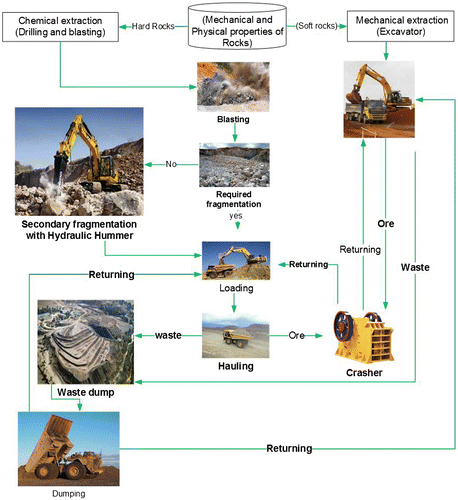
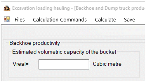
Figure 2. Shows the form Interface for estimating the volumetric capacity.

3. Productivity of an excavator and dump truck during stripping and ore extraction

The loading and transportation of limestone from Chilanga quarry to the Chilanga Cement Plant is via the excavator and dump truck combination. Whereas, a total mass of 4,000 tonnes of limestone is hauled to the plant as per daily target of production.

3.1. Calculations of the productivity backhoe excavator

In surface mining operations were the daily productivity of the ore to be hauled to the plant has been determined, it is also important to first estimate the productivity of the loader before estimating the productivity of the dump trucks when trying to optimise the fleet due to the following reasons:

	The cost of acquiring an excavator is higher than that of the dump truck to avoid high costs of acquiring the equipment.
	The productivity of the excavator determines the number of dump trucks that an excavator can accommodate within the estimated production time.

3.2. Estimated volumetric capacity of the backhoe bucket

Bucket capacity is a measure of the maximum volume of the material that can be accommodated inside the bucket of the backhoe excavator. Bucket capacity can either be measured in struck or heaped capacity. To estimate the heaped capacity, two internationally recognized standards have been adopted; these are: (i) American standard SAE J296 used for excavator, mini-excavator, and backhoe hoe bucket volumetric rating, and (ii) European standard known as the Committee of European Construction Equipment (CECE) (Patel & Prajapati, 2012). The fact that the bucket cannot be filled 100% due to the bucket fill factor, the bucket capacity is multiplied by the bucket fill factor to estimate the real volumetric capacity. In simple terms this is obtained by multiplying the bucket fill factor by the bucket size (Kennedy, 2009). An estimate using Equation (1) can be applied.(1) $$V_{\text{real}}=V_c·B_f$$(1)

where: V_c = Volumetric capacity of the backhoe bucket; B_f = Bucket fill factor.

3.3. Bulk density

Bulk density is an indicator of soil compaction. It is calculated based on the dry weight of soil divided by its volume or the specific gravity divided by the swelling factor. The volume includes that of soil particles and of pores among soil particles. Bulk density is typically expressed in g/cm³. During the estimation of truck bed tonnage of ore to be hauled, the designed equipment capacity needs to be taken into consideration. Moreover, the estimated tonnage must be compared with the manufacturer’s truck capacity, where the calculated value should be less than or equal to the fabric tonnage capacity. However, neither should the calculated value be greater than the manufacturer’s estimated tonnage capacity of the truck bed. This is important in order to secure the equipment life and its long-term usage. In addition, the mine personnel should not take advantage of the truck bed volume but the bulk density that can be calculated by using Equation (2).(2) $${\mathit{\gamma }}_e=\frac{{\mathit{\delta }}_e}{\text{Ke}}$$(2)

where: δ_e = Specific gravity; Ke = Swelling factor.

3.4. Estimated bucket bulk tonnage

The estimated bucket capacity in tonnes is estimated by multiplying the real volumetric capacity and the bulk density. Hence, Equation (3) is applied to estimate this value.(3) $$C_{\text{real}}=V_{\text{real}}·{\mathit{\gamma }}_e$$(3)

where: γ_e = Bulk density; V_real = Estimated volumetric capacity of the backhoe bucket.

3.5. Number of buckets per truck, in terms of mass

This is the number of buckets that can fit in the truck bed satisfying the conditions discussed in bulk density, Equation (4) is applied to estimate the number of buckets per truck bed.(4) $$N_b=\frac{V_{\text{bed}}}{V_{\text{real}}}$$(4)

where: V_bed = Volume of the truck bed; V_real = Estimated volumetric capacity of the backhoe bucket.

3.6. Overall efficiency of the excavator and truck combination

By definition, efficiency is the state or quality of being efficient, or able to accomplish something with a minimum amount of time and effort coupled with the required competency needed to carry out a task. In other words, the comparison of what is actually produced or performed with what can be achieved with the same consumption of resources (money, time, labor, etc.). The overall efficiency is an important factor in the determination of productivity. The efficiency is calculated by incorporating a number of factors that affect the productivity of the loaders and the hauling equipment. This parameter is very important in the optimization of fleet production as earlier shown, and can be used as a benchmarking system to help determine the quality and efficiency of the fleet production (Fuentes, 1999). This can be statistically proven in Equation (5) below:(5) $$E_{\text{ec}}=K_u·K_{\text{eo}}·K_{\text{mec}}·D_{\text{tc}}$$(5)

where: K_u = Utilization; $K_u=\frac{\text{worked time}}{\text{Total planned time}}$; K_mec = Mechanical availability; D_tc = Coefficient that takes into account the truck traffic per 5 min; K_eo = Efficiency of the machine operator.

3.7. Productivity

The productivity of a truck and loader is a major problem for mining and construction sectors. Productivity is a measure of the effectiveness in the production of goods. The productivity is expressed by the ratio of output and input. This study focuses on predicting the travel times on the haul and return portions of the truck cycle and the prediction of the interaction between the shovel and truck at the loading point (Choudhary, 2015).

3.8. Hourly productivity

Hourly productivity is a measure of the amount of minerals or waste produced within one hour of labor by the excavator or shovel. In addition, Equation (6) is applied to estimate the hourly productivity of the excavator (Fuentes, 1999).(6) $$Q=\frac{3600\times V_c·E_{\text{ec}}·B_f}{T_c·K_e}$$(6)

where: V_c = Volumetric capacity of the backhoe bucket; E_ec = Efficiency factor of the maximum usage of working hour’s routine; B_f = Bucket Factor (0.4–1); T_c = Cycle time; K_e = Swelling factor.

Note: In this case, the equation is divided by the swelling factor which means in situ productivity, where no pre-fragmentation is done. On the other hand, the hourly bulk productivity is calculated by using Equation (7) (Fuentes, 1999) as shown below:(7) $$Q=\frac{3600\times V_c·E_{\text{ec}}·B_f·K_e}{T_c}$$(7)

where: V_c = Volumetric capacity of the backhoe bucket; E_ec = Efficiency factor; B_f = Bucket Factor (0.4–1); T_c = Cycle time; K_e = Swelling factor.

Bucket Capacity of the excavator can be obtained by referring to the technical specification of the equipment supplied by the manufacturer. The swell factor is the ratio of loose dry weight per unit volume to the bench dry weight per unit volume. Bucket factor is mainly used to convert theoretical bucket capacity of excavator into actual bucket capacity. Bucket factor generally varies between 0.4 and 1 and is dependent on variables such as the height of excavation, nature of the soil and the efficiency of the operator. The term efficiency factor is used to account for actual productive operations in terms of an average number of minutes per hour that the machine will operate. For example, 50 min is considered a reasonable starting point to estimate the efficiency factor, only if the usage of the working hour routine database for the equipment is not available, of which when calculated yields an efficiency factor of 0.833 (Polanco, 2014) as shown below:$$F_e=\frac{50}{60}=0.833$$

The efficiency factor depends on a wide range of variables (i.e. the type of soil, depth of excavation, environmental condition, site conditions, operator skill etc.) in order to estimate the parameter of the bucket capacity.

The cycle time of any equipment is the total time required for an equipment to complete one cycle. However, the best way to determine the cycle time of an excavator is by monitoring aspects of the equipment operations over several periods: excavation time, swinging to the dump truck, dumping time, swinging back to the extraction face. In addition, the cleaning of the bucket is often considered during rainy seasons or when excavating wet materials and materials preparation. Besides, machinery accommodation time is also of great importance.

Productivity per shift is a measure of the amount of minerals or waste produced per shift of labor by the excavator or shovel. Equation (8) is applied to estimate the productivity per shift of the excavator.(8) $$Q_{\text{shift}}=S_d·Q$$(8)

where: Q_shift = Productivity per shift; S_d = shift duration; Q = Hourly productivity.

3.9. Daily productivity

Daily productivity is a measure of the amount of minerals or waste produced per day of labor by the excavator or shovel. In addition, Equation (9) is applied to estimate the productivity per day of an excavator.(9) $$Q_{\text{day}}=N_s·Q_{\text{shift}}$$(9)

where: Q_day = Daily productivity; N_s = Number of shifts per day; Q_shift = Productivity per shift.

3.10. Number of excavators

This is a total number of excavators or shovels that can be used considering the production schedule of the specific company per day. Its value can be calculated by using Equation (10) as shown below.(10) $$N_{\text{exw}}=\frac{V_m}{Q_{\text{day}}}$$(10)

where: V_m = Target of the require Ore at the plant per shift, day depending on the application or the amount of waste in the extraction area; Q_day = Daily productivity.

4. Calculations of the articulated dump truck productivity

4.1. Estimated volumetric capacity of the truck bed

This is calculated by multiplying the real volumetric capacity of the backhoe bucket by the assumed number of buckets that can fit in the truck bed. Its estimation is shown in Equation (11).(11) $$V_{\text{bed}}=V_{\text{real}}·N_b$$(11)

where: V_bed = Estimated volumetric capacity of the truck bed; V_real = Estimated volumetric capacity of the backhoe bucket; N_b = Assumed number of buckets.

4.2. Estimated bulk tonnage in the truck bed

The estimated bulk tonnage in the truck bed is a number of tonnes that the excavator will fill in the truck considering the manufactured capacity of the equipment. It can be calculated by using Equation (12).(12) $$M_w=C_{\text{real}}·N_b$$(12)

where: M_w = Estimated bulk tonnage in the truck bed; C_real = Estimated bucket tonnage; N_b = Assumed number of buckets.

4.3. Loading time

This is the total time that the backhoe excavator or loader takes to fill the truck bed with the required estimated number of buckets. Sometimes the number of buckets may exceed the estimated number of buckets due to the poor fragmentation of the rocks and the efficiency of the operator. This can be calculated by using Equation (13).(13) $$T_{\text{loading}}=\frac{(N_b-1)·T_l}{60}$$(13)

where: T_l = Loading duration per bucket; N_b = Assumed number of buckets.

4.4. Transportation time

This is the time taken by the dump truck to haul the material from the loading point to the dumping point; it can be calculated by using Equation (14).(14) $$T_{\text{rc}}=\frac{60·L_e}{V_{\text{rc}}}$$(14)

where: L_e = Distance of transportation from the extraction site to the dumping point; V_rc = Traveling velocity.

4.5. Dumping time

This is the time taken by the dump truck to dump the materials. However, this value can be estimated by monitoring a number of dump trucks at a dumping point. In this study, to estimate this parameter, a number dump trucks was monitored and their dumping time recorded. The recordings were summed and the average value calculated.$$t_d=0.65min$$

4.6. Returning time

The returning time is the time taken by the dump truck to travel from the dumping point to the loading point. It can be calculated by using the Equation (15) below.(15) $$T_{\text{rv}}=\frac{60·L_e}{V_{\text{rv}}}$$(15)

where: V_rv = Returning velocity.

4.7. Sampling time

Sampling time is the time taken at the sampling point to pick some samples from the dump truck proceeding to the crusher. This is done in order to control the grade of the ore being transported to the processing plant.$$t_m=0min$$

4.8. Cleaning time for the truck bed

This process is mostly done during the rainy season where the mud sticks to the truck bed and if left for a long period of time it definitely affects the productivity of the truck bed. This is also an average value that can be determined practical during the daily productive routine.$$t_l=6-7min$$

4.8.1. Maneuvering time for loading and dumping

Maneuvering time for loading and dumping is the total time that a dump truck takes maneuvering at the dumping point and at the loading point. This value also can be estimated practically during the daily productive routine. It can be calculated by using Equation (16).(16) $$t_{\text{mcd}}=t_{\text{mc}}+t_{\text{md}}$$(16)

where: T_mc = Maneuvering time for the Load; t_md = Maneuvering time for the dumping.

4.9. Cycle time for the articulated dump truck

Cycle time is the total time taken by the dump truck to make one complete cycle. This includes loading, hauling, maneuvering for dumping, dumping, returning, maneuvering for loading as well as queuing time in some cases. This can be calculated by using Equation (17).(17) $$T_c=T_{\text{loading}}+T_{\text{rc}}+t_d+T_{\text{rv}}+t_m+t_l+t_{\text{mcd}}$$(17)

4.10. Number of trips per shift for each truck

This is the estimated number of trips that a truck can attempt to haul within the shift duration or in a day. It can be calculated by using Equation (18).(18) $$N_t=\frac{T_{\text{shift}}-(T_{\text{oc}}+T_m+T_a+T_p)}{T_c}$$(18)

where: T_shift = Duration of the shift; T_oc = Time to shift changing; T_m = Resting time for lunch and snacks; T_a = resting half-time between night and day during the night this ranges between (0.66 to 0.75 h) and for a day it is 0.5 h; T_p = time lost by other causes.

4.11. Productivity of a truck per shift

This is the estimated amount of ore in tonnes that a dump truck could haul within a shift of active production. It can be calculated by using Equation (19).(19) $$Q_{\text{dump}}=N_t·V_{\text{bed}}·K_{\text{mec}}$$(19)

where: N_t = Number of trips per truck in a day; K_mec =  Mechanical availability; V_bed = Estimated volumetric capacity of the truck bed.

Note: If the extraction has been done during the rainy season, the additional parameter below must be considered K_rain = Coefficient that takes into account the delays caused by the rains.

4.12. Hourly productivity per truck

This is the estimated amount of ore in tonnes that a dump truck could haul within an hour of an active production. It can be calculated by using Equation (20).(20) $$Q_{\text{teo}}=\frac{Q_{\text{dump}}}{T_{\text{shift}}}$$(20)

where: Q_dump = Productivity of a truck per shift; T_shift = Duration of the shift.

4.13. Daily productivity per truck

This is the estimated amount of ore in tonnes that a dump truck could haul within an hour of active production. It can be calculated by using Equation (21).(21) $$Q_d=Q_{\text{dump}}·N_{\text{shift}}$$(21)

where: Q_dump = Productivity of a truck per shift; N_shift = Number of shifts.

4.14. Number of dump trucks per shift

This is the estimated number of dump trucks that can satisfy the target of the plant per shift during the peak productive time of the plant. It can be calculated by using Equation (22).(22) $$N_{\text{dumps}}=\frac{N_{\text{exw}}·Q_{\text{shift}}}{Q_{\text{dump}}}$$(22)

where: N_exw = Number of excavators; Q_shift = Productivity of an excavator per shift; Q_dump = Productivity of a dump truck per shift.

5. Match factor

The time also depends on the compatibility of loading equipment and haulage equipment (match factor) due to this parameter can be used to match the truck arrival rate to loader productivity rate or in other words it can determine the number of transport units for each loading unit. To estimate the compatibility the number of buckets per truck must be between 4 and 6, so that the choice for the capacity of the loader bucket is chosen after selecting the transport unit (Liu & Bongaerts, 2014). It can be calculated by using Equation (23).(23) $$FA=\frac{N·P·t}{n·t}=\frac{\text{total number of trucks}}{\text{number of loading units}}·\frac{\text{loading cycle time}}{\text{truck cycle time}}$$(23)

To determine the match factor (FA) it is important to consider the following variables as well: N = Total number of haulage units; n = Total number of loading units; T = Cycle time of each haulage unit; t = Cycle time of each loading unit; x = Number of haulage units per loading unit; p = Number of buckets necessary to fill a truck.

When the match factor is used to determine the suitability of a selected fleet, one must consider that the minimum fleet cost may not be the most productive. In this way, a match factor of 1.0 should not be considered ideal for the mining industry, as this corresponds to a fleet of maximum productivity. That is, a loader operating at 50% capacity may be significantly cheaper to run than another loader that operates at 100% capacity under the same conditions (Choudhary, 2015).

6. Queue length

The overall efficiency of the fleet is of key importance when determining the queuing length because if overall efficiency of the fleet is 50%, then the queuing length of the trucks will be 1 (Croft, 2016). The queuing length can be calculated by using the Equation (24).(24) $$\text{Queue length}=\left(\frac{E_{\text{ec}}}{1-E_{\text{ec}}}\right)$$(24)

Where: E_ec = Overall efficiency of the excavator and truck combination (%).

7. Basics of mathematical programming

Once the programmer has planned the program’s logic, the programmer starts writing the program instructions using the specific syntax of a programming language. In this case, Visual Basic (VB) is the programming language that was used and the Integrated Development Environment (IDE) was Visual Studio 2010.

7.1. The program code (source code)

7.1.1. Declare variables

Note: Pseudocode shown above only highlights in detail how to program the real bucket capacity by using the visual basic (VB) language.

In VB, a programmer declares constants and variables prior to their use. Variable declarations are denoted by DIM. VB supports many data types. In this class, only two data types will be employed: Integer (represents whole numbers) and Double (represents decimal numbers). In VB, the variable must be a word (contiguous set of characters, NO spaces).It must be 40 characters or less in length, and cannot use any VB Reserved words (i.e. If, Then, Else, Print, etc.).

Programming languages employ assignment statements. Though these statements resemble a mathematical equation, they are quite different. The part of the statement on the right of the equal sign is evaluated first. It’s “outcome” is then assigned to what appears to be on the left of the equal sign.

To perform mathematical calculations in VB, the following operators are used: + for addition,—for subtraction, * for multiplication, / for division and ^ for Power or Math. (Round, pow … etc.) for rounding off and powers etc.

VB uses Functions, built-in procedures that are not attached to an object that returns something. In this class, the Val Function and the Format Function were used. All data entered into a TextBox is stored as character data even if it appears numerical. To be used mathematically, numerical entries must be converted to numeric form using the Val Function.

Let’s return to the example and the program code. The first step is to create the user interface. The programmer creates one form within a project that would resemble the following:

After estimating the volumetric capacity, the header of the class was configured as shown in the code below:

This VB form has 2 Labels, 1 TextBox, and 3 GroupBox and 2 Command Buttons. Remember: save the form and save the project.

In VB, the programmer writes code to handle events. The Event-handler is a block of code that runs every time an event occurs. Now the programmer, using the Pseudocode, writes’ codes in VB syntax to handle specific events that occur. In our example, this will respond to a user’s click on the calculate button, a user’s click on the Quit button, and a change event on the TextBox. The code written for our example follows:

7.2. Testing and debugging the program

After a program is written and compiled, it must be tested and debugged. The programmer runs the program using test data to ensure the results generated by the program are accurate. If the programmer finds a debugger (error in the program), the debugger must be fixed and the test process repeated.

For this algorithm, the values were calculated manually, including using excel. The results were then compared with the test run results. The values were found to be the same, meaning that the algorithm was well programmed.

8. Results and discussions

8.1. Case study

Diesel Civil Mining (DCM) Company is the company that has been dealing with the hauling of the Chilanga limestone ore and felite for the production of different types of cement and aggregates.

Table 1 presents the parameters that are used at this quarry to determine the fleet size. The parameters in Table 2 presents the model and the capacity of the loader used for loading the hauling trucks and the parameters in Table 3 presents the capacity of the hauling trucks that are used at this quarry for the hauling of the limestone to the processing plant.

Table 1. Collected initial parameters from the DCM company

Parameters	Value	Units
Specific gravity	1.5	g/cm^3
Swelling factor	1.4	%
Shift duration	8	Hours
Number of shifts per day	2	Shifts
Equipment utilization	83.3	%
Mechanical availability	84.4	%
Volume of the bucket	2.2	m3
Capacity of the dump truck bed	30	Tonnes
Transportation velocity	30	km/hour
Operator’s efficiency	97	%
Truck traffic per five minutes	95	%
Transportation distance	8.7	km
Sampling time	0	Minutes
Truck bed cleaning time	0	Minutes
Maneuvering time	4	Minutes
Dumping time	0.65	Minutes
Shift changing time	0.25	Hours
Maximum usage of the work routine Ku	82	%
The bucket fills factor Bf	95	%

Table 2. Technical characteristics of the backhoe excavator collected from DCM

Code	Machine	Model	Capacity
EX01	Hydraulic excavator	Hyundai	2.2 m^3
EX02	Hydraulic excavator	Hyundai	1.16 m^3

Table 3. Technical characteristics of the dump trucks Scania G380 collected from DCM

Code	Model	Parameter	Capacity and units
TR01	Scania G380	Tonnage capacity	30 tonnes
		Volume of the truck bed	28 m^3

During the calculation of the fleet size, it is of great importance to know some of the important parameters that can be used as initial data for the calculation of the fleet size. Figure 3 shows an interface of some of the initial parameters that were used to determine the fleet size of the case study.

Figure 3. Shows the initial data on the input interface.

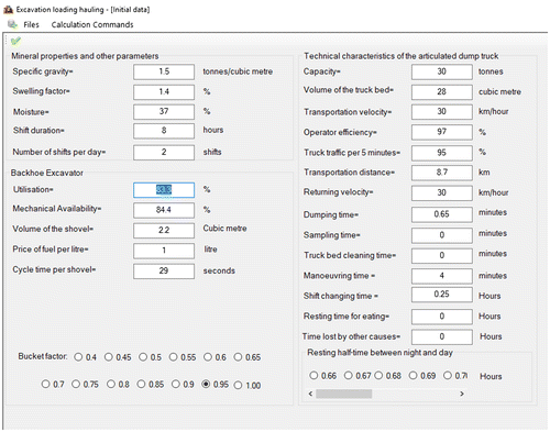
Figure 4 shows the results of the fleet size that was obtained by using the formulas discussed in this paper earlier on which has been embedded in a small computer application.

Figure 4. Shows the results of the fleet on the output interface.

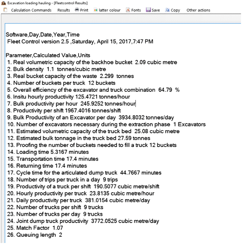
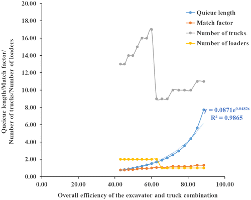
According to Figure 5 and the parameters shown in Figure 3, it is clearly illustrated that the optimal overall efficiency of 65.1% would be ideal for the reduction of the queuing length by applying the model discussed in this paper. Based on the characteristics of this quarry, the optimum number of the loader is 1 and the optimum number of trucks should be 9.

Figure 5. The relation of the overall efficiency to other fleet optimization parameters.

9. Conclusion

During the calculation of the fleet in Surface Mining, the number of loaders and its productivity must be determined first, whereas, the truck productivity must be calculated based on the productivity of the loaders.

The model examined in this paper can help improve the loader per truck match factor. As it can as well help to reduce the queuing length at the loading point. Based on the characteristics of the case study, a match factor of 1.07 was obtained with the queuing length of 2 trucks per shovel. Using this model, it was found that there was an excess of two trucks being used at this quarry, which led to an increase in queuing at the point of loading. For this reason, it is very important to consider the productivity of an excavator or loader in order to calculate the optimal fleet in surface mining and quarries.

Funding

The authors received no direct funding for this research.

Acknowledgements

I am highly thankful to University of Zambia, School of Mines and Chilanga Cement, Diesel Civil Company for their remarkable support for the collection of data for finalizing this manuscript. I would like to express my gratitude also towards Mr Cryton Phiri from University of Zambia, School of Mines Department of Geology for helping us to proof read this manuscript.

Additional information

Notes on contributors

Marsheal Fisonga

Marsheal Fisonga received a bachelor degree in Mining Engineering from The Higher Institute of Mining and Metallurgy of Moa (ISMM), Holguin, Cuba. I am staff development fellow in the Department of Mining Engineering at The University of Zambia School of Mines. Currently I am reading Master of Science in geotechnical engineering at The Institute of Geotechnical Engineering, Southeast University, Nanjing, China. My research interest are: applied geotechnical engineering, geotechnical simulation, mine planning, application of mining softwares, geostatistics, mathematical programming, mine surveying, deformation analysis applied to subsidence and slopes, mine transportation, and drilling and blasting. I am a registered graduate engineer with the Engineering Institution of Zambia. I am the first author of the publication titled “Burden estimation using relative bulk strength of explosive substances”.

References

- Choudhary, R. P. (2015). Optimization of load – Haul – Dump mining system by Oee and match factor for surface mining. International Journal of Applied Engineering and Technology, 5(2), 96–102.
- Croft, C. (2016). Process improvement fundamentals. Retrieved from Lynda.com: http://www.chriscroft.co.uk/?v=0f177369a3b7
- Fuentes, O. B. (1999). Mining machineries and installation. Moa: ISMM.
- Kennedy, E. B. B. A. (2009). Surface mining. Littleton, CO: Society for Mining, Metallurgy, and Exploration, Inc. (SME). Retrieved from www.smenet.org
- Liu, J., & Bongaerts, J. C. (2014). Mine planning and equipment selection. Mine Planning and Equipment Selection. doi:10.1007/978-3-319-02678-7
- Patel, B., & Prajapati, J. (2012). Evaluation of bucket capacity, digging force calculations and static force analysis of mini hydraulic backhoe excavator. Machine Design, 4(1), 59–66 http://standards.globalspec.com/std/1856598/sae-j296
- Polanco, A.R. (2014) Notes of surface mining. Moa. Retrieved from http://docplayer.net/22851170-Improving-productivity-of-mining-machinery-through-total-productive-maintenance.html