Coarse grain automatic differentiation: A practical approach to fast and exact computation of first and second order derivatives in software

Abstract

The evaluations done by a program at runtime can be modeled by computational Directed Acyclic Graphs (DAGs) at various abstraction levels. Applying the multivariate chain rule on those computational DAGs enables the automation of total derivatives computation, which is exploited at a fine-grain level by Automatic Differentiation (AD). Coarse Grain Automatic Differentiation (CGAD) is a framework that exploits this principle at a higher level, leveraging on software domain model. All nodes in the computational DAG are responsible for computing local partial derivatives with respect to their direct dependencies while the CGAD framework is responsible for composing them into first- and second-order total derivatives. This separation of concerns between local and global computations offers several key software engineering advantages: it eases integration, makes the system decoupled and inherently extensible, and allows hybrid differentiation (i.e. connecting derivatives from different sources using different calculation methods and different languages in the same evaluation). Additionally, the nodes can take advantage of local symbolic differentiation to significantly speed up total derivatives computation, compared to traditional differentiation approaches. As a concrete application of this methodology to a financial software context, we present a Java implementation that computes the premiums and 82 first- and second-order total derivatives of 2000 call options in 262 milliseconds, with a time ratio of 1:2.2 compared to premiums alone.

Keywords:

• cgad
• ad
• automatic differentiation
• chain rule
• abstraction level
• modularity
• hybrid
• parallel
• decouling
• differentiation

Public Interest Statement

Computing first order derivatives in software is not an easy task. At second order it is even worse. So far, choosing one differentiation method was a trade-off between responding to user experience concerns (precision, speed) and responding to software engineering concerns (decoupling, integrability $\dots$). This articles describes a new way to compute first and second order derivatives, called Coarse Grain Automatic Differentiation, located at the crossroads of functional, software and performance engineering, that responds to both. It allows hybrid differentiation i.e. connecting derivatives from different sources using different calculation methods and different languages in the same evaluation. And, when combined with local symbolic differentiation, it can run significantly faster than traditional differentiation approaches.

1. Introduction

Derivatives are fundamental in many numerical activities, from physics to economics, to predict an evolution, speed up a computation or help to make a decision. In finance, the total derivatives of instrument prices with respect to their underlying parameters are called Greeks. They are instrumental for risk management and highly desirable for the quick Taylor approximation of prices when underlying parameters change (either in response to real-time feed events or simulation scenarios).

Unfortunately, every classical methods for calculating derivatives in software comes with its own drawbacks. And to make matters worse, those drawbacks get magnified when computing second-order derivatives. Choosing one differentiation method is usually a trade-off between responding to user experience concerns (precision, speed) and responding to software engineering concerns (decoupling, integrability $\dots$).

(1)	Symbolic differentiation (i.e. coding the derivative formulas) addresses user experience concerns as it is both exact and fast. It works very well on small blocks of code, however it becomes impractical on large codes as derivative formulas tend to grow exponentially making the code too complex to write and maintain (Duché & Galilée, 2017). In addition, total derivative formulas are global quantities that contain local partial derivatives from all calculation modules, linked together by the chain rule. So coding total derivative formulas unfortunately induces coupling between all calculation modules.
(2)	Finite difference approach consists in slightly bumping one factor, repeating the calculation and approximating a derivative by a difference quotient. It addresses software engineering concerns as it is simple to code and induces no coupling. However, it does not meet user experience requirements as it is often highly inefficient and potentially inaccurate (Naumann, 2012).
(3)	AD is an increasingly popular alternative that is exact up to machine precision and efficient at first order in specific cases. It comes in two modes: forward mode and adjoint mode. The forward mode is efficient when the function has one input and a large number of outputs while the adjoint mode (commonly called AAD) is efficient when the function has a large number of inputs and one output as it is typically the case in finance (Giles & Glasserman, 2006). However, at second order, the speed advantage of AD compared to finite difference is lost as it becomes linear in the number of inputs (Henrard, 2011b). Additionally, AD integration is a time-consuming process as it requires a very bottom-up approach (Henrard, 2011b).

CGAD is a new method to compute first- and second-order total derivatives that aims at responding to user experience concerns as well as software engineering concerns.

2. Computational DAGs in software

2.1. Computational DAG at assembler level

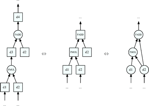
It is possible to draw the data flow diagram (DFD) of a program at runtime. This is accomplished by monitoring numbers written and read by a processor (Griewank & Walther, 2008) as in Figure 1 - left part where data are displayed in boxes and assembler instructions in circles.

By letting arrows implicitly represent assembler instructions and labeling data with the assembler instruction that output them, the DFD is semantically equivalent to the tree in Figure 1 - middle part.

Since numbers in memory are typically used as the inputs of several instructions, the tree can be further compacted and represented as the DAG in Figure 1 - right part.

Figure 1. Computational DAG at assembler level (left part), DFD as a tree (middle part), and DFD as a DAG (right part).

The AD community has explored a way to differentiate at this instruction level and built a prototype called ADAC (Automatic Differentiation of Assembler Code; Gendler, Naumann & Christianson, 2007).

2.2. Computational DAG at programming language level

The assembler instructions that are executed at runtime are typically generated by a compiler from a code written in a higher level programming language. Such a programming language offers a way for the developer to control the instructions and memory access generated for the processor via arithmetic operators, intrinsic mathematical functions (sqrt, exp, ln $\dots$), variable scopes, and caching mechanisms.

Therefore, when coding an evaluation program, the developer is actually giving hints (not totally controlling as the compiler and the processor have the final say) for the topological ordering in which a data flow DAG should be constructed, traversed, and discarded at runtime to produce the desired output.

Considering those arithmetic operators and intrinsic mathematical functions, we can draw a higher abstraction-level DAG representation for the same program runtime evaluation. The nodes no longer correspond to assembler instruction outputs but to the assignment of input variables and programming language function results (Naumann, 2012).

As a concrete example from the financial world, consider a program to evaluate European call options. A European call option C is a contract giving the right to buy a stock S at an agreed price K (called the strike), on a specified future maturity date T. Such option is typically valued using the Black formula that requires as additional inputs the stock volatility V and a risk-free interest rate Z (Black, 1976):$$\begin{array}{c}\hfill C=\text{DF}·(F\mathrm{\Phi }(d_1)-K\mathrm{\Phi }(d_2))\end{array}$$

where $\text{DF}=e^{-ZT}$;$F=\frac{S}{\mathit{DF}}$; $d_1=\frac{ln(\frac{F}{K})}{V\sqrt{T}}+\frac{V\sqrt{T}}{2}$; $d_2=\frac{ln(\frac{F}{K})}{V\sqrt{T}}-\frac{V\sqrt{T}}{2}$ and $\mathrm{\Phi }$ stands for the cumulative distribution function of the standard normal law.

The runtime computational DAG of an implementation of the Black formula in a classical programming language like C$++$ or Java is given in Figure 2.

Figure 2. Computational DAG at programming language level.

Figure 3. Computational DAG with framed domain model functions.

AD typically works on this abstraction-level computational DAG by providing and composing the derivatives of the arithmetic operators and intrinsic mathematical functions of the programming language (Bischof & Haghighat, 1996; Naumann, 2012).

2.3. Computational DAG at domain model level

When designing complex software, developers typically build a domain model to represent meaningful concepts, relations, and behaviors in the application domain (Fowler, 2002). The arithmetic operators and intrinsic mathematical functions of the programming language serve as basic materials to implement the high abstraction-level functions of the domain model.

It is therefore possible to draw a even higher abstraction-level computational DAG representation of the same program runtime evaluation by considering only domain model functions. The nodes no longer correspond to single assignments of programming language function results but to single assignments of domain model function results.

For example, for the same runtime evaluation of Figure 2, it is possible to arbitrarily only consider the high-level domain model functions framed in Figure 3, to get the domain model computational DAG of Figure 4.

Domain model computational DAGs are of paramount importance in software as they illustrate at runtime the domain model built at design-time, as shown in Figure 4.

Figure 4. (Left) Computational DAG at domain model level; (Right) UML class diagram of software domain model.

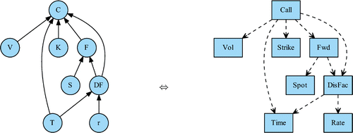
CGAD works on this higher abstraction-level computational DAG by composing the local partial derivatives provided by the domain model functions.

2.4. Computational DAGs equivalence

Figure 5. Different abstraction-level computational DAGs and their associated differentiation technique.

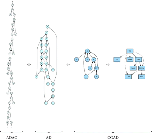
As illustrated by Figure 5, several computational DAGs correspond to the same evaluation at runtime, seen from different perspectives i.e. depending on the set of functions considered: assembler instructions, programming language functions or domain model functions. And each of those different abstraction-level computational DAGs has its associated way of computing total derivatives.

3. Total derivatives on a computational DAG

3.1. Multivariate chain rule

In Leibniz’s notation, if a variable z directly depends on a variable y, which itself depends on a variable x: z(y(x)), the first order univariate chain rule states that:$$\begin{array}{c}\hfill \frac{\text{d}z}{\text{d}x}=\frac{\text{d}z}{\text{d}y}·\frac{\text{d}y}{\text{d}x}\end{array}$$

In the multivariate case, if a variable z directly depends on n variables $y_1,\dots ,y_n$, which themselves all depend on a variable x: $z\left(y_1\left(x\right),\dots ,y_n\left(x\right)\right)$, it is necessary to distinguish partial from total derivatives:

• Partial derivatives with respect to one variable consider that the other variables are constant. They are noted: ${\left(\frac{\mathit{\partial }z}{\mathit{\partial }{y}_i}\right)}_{\left\{y_j\mid j\in [[1,n]],j\ne i\right\}}$ or simply $\frac{\mathit{\partial }z}{\mathit{\partial }{y}_i}$

• Total derivatives with respect to one variable take into account indirect dependencies between the variables. They are noted: $\frac{\text{d}z}{\text{d}x}$

The first-order multivariate chain rule is given by Formula (1):(1) $$\begin{array}{c}\hfill \frac{\text{d}z}{\text{d}x}=\sum _{i=1}^n\frac{\mathit{\partial }z}{\mathit{\partial }{y}_i}·\frac{\text{d}{y}_i}{\text{d}x}\end{array}$$(1)

To state the second-order multivariate chain rule, we need to consider another variable u that can either be identical to or distinct from x (both cases leading to the same generic formula).

If a variable z directly depends on n variables $y_1,\dots ,y_n$, which themselves all depend on two variables x and u: $z(y_1(x,u),\dots ,y_n(x,u))$, by differentiating Formula (1) with respect to u and by the symmetry of second derivatives, we get Formula (2) which is the second order multivariate chain rule:$$\begin{array}{c}\hfill \frac{{\text{d}}^{2}z}{\text{d}x\text{d}u}=\frac{{\text{d}}^{2}z}{\text{d}u\text{d}x}=\frac{\text{d}}{\text{d}u}\left(\frac{\text{d}z}{\text{d}x}\right)=\frac{\text{d}}{\text{d}u}\left(\sum _{i=1}^n\frac{\mathit{\partial }z}{\mathit{\partial }{y}_i}·\frac{\text{d}{y}_i}{\text{d}x}\right)\end{array}$$

applying the sum and then the product differentiation rules:$$\begin{array}{c}\hfill \frac{{\text{d}}^{2}z}{\text{d}x\text{d}u}=\sum _{i=1}^n\frac{\text{d}}{\text{d}u}\left(\frac{\mathit{\partial }z}{\mathit{\partial }{y}_i}\right)·\frac{\text{d}{y}_i}{\text{d}x}+\sum _{i=1}^n\frac{\mathit{\partial }z}{\mathit{\partial }{y}_i}·\frac{\text{d}}{\text{d}u}\left(\frac{\text{d}{y}_i}{\text{d}x}\right)\end{array}$$

yet, as $\frac{\mathit{\partial }z}{\mathit{\partial }{y}_i}$ depends on the same variables as z, by applying the first order multivariate chain rule with respect to u, we get:$$\begin{array}{c}\hfill \frac{\text{d}}{\text{d}u}\left(\frac{\mathit{\partial }z}{\mathit{\partial }{y}_i}\right)=\sum _{j=1}^n\frac{\mathit{\partial }}{\mathit{\partial }{y}_j}\left(\frac{\mathit{\partial }z}{\mathit{\partial }{y}_i}\right)·\frac{\text{d}{y}_j}{\text{d}u}=\sum _{j=1}^n\frac{{\mathit{\partial }}^{2}z}{\mathit{\partial }{y}_i\mathit{\partial }{y}_j}·\frac{\text{d}{y}_j}{\text{d}u}\end{array}$$

thus:$$\begin{array}{c}\hfill \frac{{\text{d}}^{2}z}{\text{d}x\text{d}u}=\sum _{i=1}^n\sum _{j=1}^n\frac{{\mathit{\partial }}^{2}z}{\mathit{\partial }{y}_i\mathit{\partial }{y}_j}·\frac{\text{d}{y}_i}{\text{d}x}·\frac{\text{d}{y}_j}{\text{d}u}+\sum _{i=1}^n\frac{\mathit{\partial }z}{\mathit{\partial }{y}_i}·\frac{{\text{d}}^2{y}_i}{\text{d}x\text{d}u}\end{array}$$

3.2. Multivariate chain rule on a computational DAG

Consider $G=(V,E)$, a computational DAG of any abstraction level with V and E its vertices and edges.

Note that:

• A vertex $v\in V$ directly depends on another vertex $w\in V$ or, equivalently, w is a direct dependency of v, if there is a directed edge in E pointing from w to v.

• A vertex $v\in V$ indirectly depends on another vertex $w\in V$ or, equivalently, w is an indirect dependency of v, if v is reachable from w with no directed edge in E pointing from w to v.

• The indegree $n_v$ of a vertex $v\in V$ is the number of vertices on which v directly depends (if $n_v=0$, then v is a source vertex).

• The inverse adjacency list of a vertex $v\in V$ corresponds to the set of vertices on which v directly depends or, equivalently, to the list of direct dependencies of v. Its cardinality is $n_v$.

Definition 1

Let z be a vertex in a computational DAG $G=(V,E)$, $n_z$ be its indegree and $\left(y_1,\cdots ,y_{n_z}\right)$ be its inverse adjacency list. We call local partial derivatives of z the quantities:$$\begin{array}{c}\hfill {\left(\frac{\mathit{\partial }z}{\mathit{\partial }{y}_i}\right)}_{\left\{y_j\mid j\in [[1,n_z]],j\ne i\right\}}\text{or simply}\frac{\mathit{\partial }z}{\mathit{\partial }{y}_i},i\in [[1,n_z]]\end{array}$$

If a vertex $z\in V$ directly or indirectly depends on a vertex $x\in V$ (i.e. if it exists a directed path from x to z), then a deviation $\mathrm{\Delta }x$ in x causes a deviation $\mathrm{\Delta }z$ in z (Bauer, 1974).

Definition 2

Let x and z be two vertices in a computational DAG $G=(V,E)$. We call total derivative of z with respect to x the quantity:$$\begin{array}{c}\hfill \frac{\text{d}z}{\text{d}x}=\underset{\mathrm{\Delta }x\to 0}{lim}\frac{\mathrm{\Delta }z}{\mathrm{\Delta }x}\end{array}$$

A fundamental property of total derivatives on computational DAGs is given by Bauer in Bauer (1974):

Property 1

If a vertex $z\in V$ does not directly nor indirectly depend on a vertex $x\in V$ (i.e. if there is no directed path from x to z), then $\frac{\text{d}z}{\text{d}x}=0$

Even if this fundamental property sounds like an obvious result, it is important to note that it is specific to computational DAGs and not transposable to standard mathematics where equalities go both ways and functions can be implicitly defined.

A direct corollary of Property 1 is:

Corollary 1

If a vertex $z\in V$ directly or indirectly depends on a distinct vertex $x\in V$ then, as G is acyclic, x cannot in turn depend on z and therefore $\frac{\text{d}x}{\text{d}z}=0$

From Property 1 and assuming differentiability on all vertices, the first- and second-order multivariate chain rule can be extended to computational DAGs yielding Formulas (3) and (4).

At first order:$$\begin{array}{c}\hfill \forall (z,x)\in V^2,\frac{\text{d}z}{\text{d}x}=\left\{\begin{array}{cc}1\hfill & \text{if}z=x\hfill \\ {\sum }_{i=1}^{n_z}\frac{\mathit{\partial }z}{\mathit{\partial }{y}_i}·\frac{\text{d}{y}_i}{\text{d}x}\hfill & \text{if}z\ne x\hfill \end{array}\right.\end{array}$$

or equivalently, applying Corollary 1 on the direct dependencies of x when $z=x$:(2) $$\begin{array}{c}\hfill \forall (z,x)\in V^2,\frac{\text{d}z}{\text{d}x}=1_{[z=x]}+\sum _{i=1}^{n_z}\frac{\mathit{\partial }z}{\mathit{\partial }{y}_i}·\frac{\text{d}{y}_i}{\text{d}x}\end{array}$$(2)

At second order:(3) $$\begin{array}{cc}\hfill \forall (z,x,u)\in V^3,\frac{{\text{d}}^{2}z}{\text{d}x\text{d}u}& =\sum _{i=1}^{n_z}\sum _{j=1}^{n_z}\frac{{\mathit{\partial }}^{2}z}{\mathit{\partial }{y}_i\mathit{\partial }{y}_j}·\frac{\text{d}{y}_i}{\text{d}x}·\frac{\text{d}{y}_j}{\text{d}u}+\sum _{i=1}^{n_z}\frac{\mathit{\partial }z}{\mathit{\partial }{y}_i}·\frac{{\text{d}}^2{y}_i}{\text{d}x\text{d}u}\hfill \end{array}$$(3)

3.3. Recursive definition of total derivatives on a computational DAG

As highlighted in Formula (5), Formulas (3) and (4) exhibit a joint-multivariate recursive definition of all first- and second-order total derivatives in a computational DAG $G=(V,E)$ equipped with some topological ordering:

If we know the first- and second-order total derivatives of all the direct dependencies $\left(y_1,\cdots ,y_{n_z}\right)$ of a vertex z with respect to all vertices in V and pairs of vertices in $V^2$:$$\begin{array}{c}\hfill \left\{\frac{\text{d}{y}_i}{\text{d}x}\mid x\in V,i\in [[1,n_z]]\right\}\cup \left\{\frac{{\text{d}}^2{y}_i}{\text{d}x\text{d}u}\mid (x,u)\in V^2,i\in [[1,n_z]]\right\}\end{array}$$

then it is possible to combine them with the first- and second-order local partial derivatives of z:$$\begin{array}{c}\hfill \left\{\frac{\mathit{\partial }z}{\mathit{\partial }{y}_i}\mid i\in [[1,n_z]]\right\}\cup \left\{\frac{{\mathit{\partial }}^{2}z}{\mathit{\partial }{y}_i\mathit{\partial }{y}_j}\mid (i,j)\in {[[1,n_z]]}^2\right\}\end{array}$$

to get the first- and second-order total derivatives of z with respect to all vertices in V and pairs of vertices in $V^2$:$$\begin{array}{c}\hfill \left\{\frac{\text{d}z}{\text{d}x}\mid x\in V\right\}\cup \left\{\frac{{\text{d}}^{2}z}{\text{d}x\text{d}u}\mid (x,u)\in V^2\right\}\end{array}$$

The recursive definition is seeded on all source vertices s in V (where $n_s=0$), by Formulas (3) and (4) that reduce to:$$\begin{array}{c}\hfill \forall x\in V,\frac{\text{d}s}{\text{d}x}=1_{[s=x]}\text{and}\forall (x,u)\in V^2,\frac{{\text{d}}^{2}s}{\text{d}x\text{d}u}=0.\end{array}$$  

4. CGAD

CGAD is a framework that exploits Formula (5) on the high-level domain model computational DAGs of the software industry.

All nodes are solely responsible for computing local partial derivatives with respect to their direct dependencies while total derivatives computation is delegated to a Multivariate Chain Rule Engine (MCRE) as illustrated in Formula (6).

To compute first- and second-order total derivatives, the MCRE does not require more than the natural topological ordering traversal of the computational DAG that computes values.

4.1. CGAD software engineering advantages

The sharp division of roles between local and global computations in CGAD is a structuring separation of concerns (Dijkstra, 1982) that offers several key software engineering advantages:

4.1.1. Hybrid differentiation

The encapsulation of local partial derivative computation methods inside each node allows hybrid differentiation i.e. connecting derivatives from different sources using different calculation methods and different languages in the same evaluation. Each node’s implementer can independently choose the most appropriate method to generate its local partial derivatives: symbolic differentiation, finite difference, AD, or even CGAD at a finer local grain.

4.1.2. Extensibility

Integrating CGAD in software makes the system inherently extensible. The code is made of self-contained blocks: the nodes, that encapsulate their local partial derivatives computation. The nodes are coded once and can be composed afterwards in any way. Any new node composition gives a new computational DAG at runtime, whose total derivatives are automatically calculated by the MCRE.

4.1.3. Flexibility

The MCRE can work on any abstraction-level computational DAG. However, as stated in Bischof and Haghighat (1996), fine-grained computational DAGs (at the programming language level) do not scale and become impractical on large programs. Conversely, excessively increasing the grain sizes leads to code complexity that goes beyond the mathematical and software engineering skills of the developers (i.e. the code complexity they are able to write, test, debug and maintain).

CGAD offers the flexibility to chose the most appropriate granularity to the context. This choice will typically be a compromise between the scalability and integrability of coarse grains on the one hand and the decoupling and code simplicity of fine grains on the other hand.

4.1.4. Integrability

CGAD offers two integration advantages:

(1)	At a global scale, the hybrid characteristic of CGAD enables transparent integration of different computation modules.
(2)	At a local scale, the flexible characteristic of CGAD enables cost-effective top-down integration inside a computation module. This is a competitive advantage compared to fine-grained AD that requires time-consuming bottom-up integration (Henrard, 2011b).

4.1.5. Decoupling

CGAD brings to light domain model computational DAGs. This strengthens software modularity and clears up module dependencies. By delegating global computations to a separated MCRE, it allows full decoupling between the implementation modules, that only perform local computations.

4.1.6. Common language

Domain Driven Design (DDD) is a software development approach that is well adapted to the complex domains of the software industry. It leads developers and domain experts to build (and constantly use) a common language describing the domain model called the “Ubiquitous Language” (Evans, 2004).

CGAD naturally spurs developers and domain experts to work together in DDD mode: it supports the domain model and the “Ubiquitous Language” by placing domain model computational DAGs at the heart of the development process: in specifications, code and results.

4.2. CGAD compelling combinations

As mentioned in Section 4.1.1, the hybrid characteristic of CGAD allows any combination of local partial derivatives computation methods in the same evaluation. However combinations focused on symbolic differentiation and AD have very appealing arguments for user experience: precision and speed.

4.2.1. Precision

An interesting combination enabled by CGAD is to get all nodes appearing in a computational DAG to use only symbolic differentiation or AD to compute their local partial derivatives. In such a situation, each node provides the MCRE with local partial derivatives that are exact up to machine precision. The associativity and commutativity of the summations in Formula (6) ensures that the total derivatives computed by the MCRE are also exact up to machine precision.

4.2.2. Speed

As shown in the implementation described in Section 5, CGAD can outperform AD and finite difference by doing local symbolic differentiation inside all nodes of a computational DAG. The substantial performance gain typically comes from:

• Mathematical simplification Mathematical expressions of local partial derivatives can comprise significant simplifications that are well exploited by computer algebra systems. Symbolic differentiation, unlike finite difference and fine-grained AD (Griewank & Walther, 2008), can exploit those simplifications to significantly reduce the algorithmic complexity of local partial derivative calculations (Henrard, 2011a).

• Implicit function differentiation A node in a computational DAG can depend on other nodes through a set of implicit equations. Those implicit equations are usually solved by an iterative method that can be time-consuming. In such a case, the implicit function theorem gives the explicit expressions of the node’s first order local partial derivatives which can, in turn, be differentiated explicitly (Kaplan, 1952) to get its second order local partial derivatives. This method is considerably faster than fine-grained AD, that differentiates inside the solver, and finite difference, that runs the time-consuming solver several times (Henrard, 2011).

• Local computation reuse Symbolic differentiation makes it possible to fruitfully reuse local variables of the value computation. This can reduce the added complexity of the local partial derivatives computation up to a fraction of the node’s value complexity. As a basic illustration of reuse, if the node’s value is $z=x^n$, a $O(log(n))$ operation, then $\frac{\mathit{\partial }z}{\mathit{\partial }x}=n{x}^{n-1}$ and $\frac{{\mathit{\partial }}^{2}z}{\mathit{\partial }{x}^2}=n(n-1)x^{n-2}$ may still appear as having $O(log(n))$ runtime complexity. Since z is known, however, the derivatives can be much more efficiently computed as $\frac{\mathit{\partial }z}{\mathit{\partial }x}=\frac{n}{x}·z$ and $\frac{{\mathit{\partial }}^{2}z}{\mathit{\partial }{x}^2}=\frac{n-1}{x}·\frac{\mathit{\partial }z}{\mathit{\partial }x}$, reducing complexity to O(1).

4.3. CGAD optimization options

It is possible to increase CGAD algorithmic efficiency by exploiting parallelism in Formula (6), total derivatives sparsity and lazy initialization.

Those three optimizations are used in the financial Java implementation described in Section 5.

4.3.1. Parallelism

The local partial derivatives computations done in the nodes do not depend on the total derivatives computations done by the MCRE. Thus, the MCRE can be executed in a parallel computation pipeline acting as a transparent consumer on the local partial derivatives and following a similar topological ordering traversal of the computational DAG.

4.3.2. Sparsity

Given the sparse characteristic of total derivatives in a computational DAG resulting from Property 1 and Corollary 1, CGAD can gain in efficiency by maintaining only non-null total derivatives.

In such case, the MCRE performs two separate steps on each node z during the topological ordering traversal of the computational DAG, as highlighted in Formula (7):

(1)	A creation step in which new first- and second-order total derivatives are created on z.
(2)	A composition step in which the total derivatives of z’s direct dependencies $\left(y_1,\cdots ,y_{n_z}\right)$ are multiplied by z’s corresponding first-order local partial derivatives.

The set of non-null total derivatives is then gradually enriched by the MCRE on each node along the topological ordering traversal of the computational DAG.

4.3.3. Lazy initialization

In practice, users are often interested in a subset of all possible non-null total derivatives. For instance, in software with a graphical user interface, the subset of total derivatives to display might depend on the view chosen by the user.

CGAD can take advantage of such a situation by implementing the lazy initialization idiom (Martin, 2008) on total derivatives:

(1)	The user specifies, at runtime, a set of first- and second-order total derivatives creation criteria.
(2)	Those criteria are checked on each node during the computational DAG traversal.
(3)	The total derivatives of the node are only created if they match the criteria.

Lazy initialization of total derivatives is possible as the recursive definition exhibited in Formula (5) can be narrowed to first-order total derivatives with respect to all nodes in any subset $D_1\subset V$ and second-order total derivatives with respect to all pairs of nodes in any subset $D_2\subset {D_1}^2$, as shown in Formula (7).

 

5. Implementation in financial software

5.1. Context

In this section, we see how various requirements of the finance industry induce strong constraints on computational DAGs and total derivatives computation for software builders willing to propose fast evaluations and good time to market.

5.1.1. Pricing

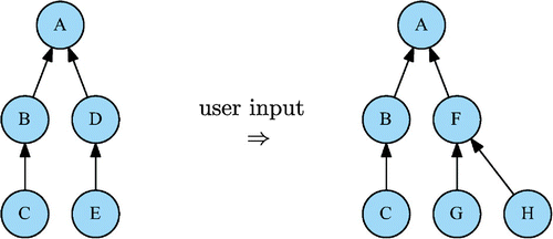
In a pricing screen, the financial product and the evaluation parameters are defined at runtime in reaction to the user input. The corresponding computational DAG cannot remain static and should permit dynamic modifications (Figure 6).

Figure 6. Dynamic computational DAG.

5.1.2. Portfolio management

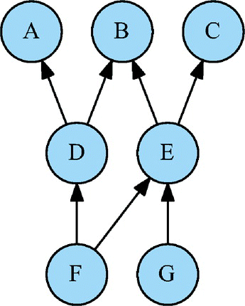
A financial product is not evaluated in isolation. Financial product transactions are gathered in a portfolio and evaluated together in a portfolio management screen. The different products in the portfolio typically share common features and market data that might take time to compute and calibrate. Significant performance gains can be achieved by allowing the corresponding computational DAGs to share common nodes resulting in one multi-sinked DAG (Figure 7).

Figure 7. Multi-sinked computational DAG.

5.1.3. Continuous evaluations

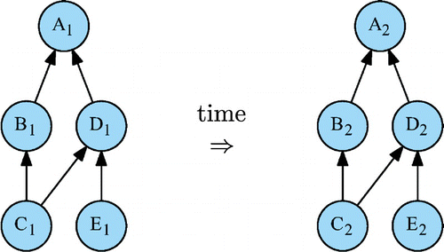
A financial product is not evaluated only once. A portfolio management screen is continuously updated by real-time market data feeds and user scenarios. Significant performance gains can be achieved by keeping the computational DAG in memory and traversing it again when the source node values change; either in response to real time feed events or simulation scenarios (Figure 8).

Figure 8. Reused computational DAG.

5.1.4. Proxy evaluations

Continuous evaluation in a portfolio management screen can be impossible to put in place if the computation time is bigger than the expected refresh cycle. A pragmatic trade-off used by finance practitioners is to set a longer full evaluation refresh cycle in addition to a faster but less accurate approximation when underlying parameters change. These faster computations typically use a Taylor series expansion that requires fast and exact first- and second-order total derivatives. Such fast proxy evaluations are also used by finance practitioners on simulation scenarios (Figure 9).

Figure 9. Proxy evaluation.

5.1.5. Intermediary risks

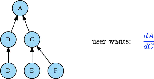
Finance practitioners sometimes hedge with derivative products that embed several risk factors. For instance, it is possible to hedge an option with a forward to simultaneously get rid of spot risk and dividend risk. The number of forward contracts to buy or sell is given by the total derivatives of the option node with respect to the forward node (which is an internal node in the computational DAG). It should therefore be possible to compute total derivatives with respect to internal nodes in the computational DAG (Figure 10).

Figure 10. Intermediary risk in a computational DAG.

5.1.6. New financial products

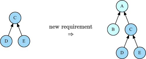
The finance industry constantly creates new products based on existing ones. For instance, options on futures, options on swaps or swaps on option payoffs. They are called derivatives as their values derives from the value of the underlying products on which they are built. The computational DAGs of those new products are built upon the computational DAGs of their underlyings. Consequently, the sinks of today’s computational DAGs should not be frozen as they can become internal nodes of tomorrow’s computational DAGs (Figure 11).

Figure 11. Up-growing computational DAG.

5.1.7. Model fine-tuning

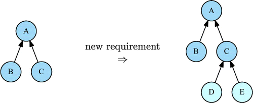
When an old and faithful model has shown its limits in representing the reality of market behaviors, the finance industry has a pragmatic tendency to keep it and fine tune it by giving it additional degrees of freedom to stick to the market. For instance make the volatility of a stock depend on the option moneyness $(M=\frac{K}{S})$. The computational DAGs of those fine-tuned models contain additional nodes at their bottom, corresponding to the new degrees of freedom. Consequently the sources of today’s computational DAGs should not be frozen as they can become internal nodes of tomorrow’s computational DAGs (Figure 12).

Figure 12. Down-growing computational DAG.

5.1.8. Openness

Financial practitioners want to be able to plug their own local evaluation model inside a global evaluation framework. This implies that part of the computational DAG can be provided by an external library (Figure 13).

Figure 13. Open computational DAG.

5.2. Specification

Our objective is to compute the premium and certain Greeks of a 18 months maturity, 34 EUR strike, European call option C on a 35 EUR stock S using the Black Formula (1976). As mentioned in Section 2.2, the Black formula requires the stock volatility V and a risk-free interest rate Z as additional inputs.

The risk-free interest rate Z is not directly observable. It is interpolated on a zero-coupon yield curve $C{Z}_i$ that is an implicit function of coupon-bearing instrument quoted rates $Q{R}_i$:

The volatility V also is not directly observable. It is interpolated on a two-dimensional surface of quoted volatilities $Q{V}_i$ for different option moneyness and maturities: The user is interested in the 82 first- and second-order Greeks of Table 1.

Table 1. Requested greeks

5.3. Implementation

We describe a CGAD implementation written in Java, that satisfies the constraints on computational DAGs and total derivatives computation of Section 5.1. Our description uses standard programming constructs found in mainstream object oriented languages for easy integration in a wide variety of existing codebases.

5.3.1. Framework design

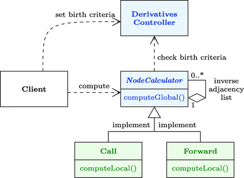
As illustrated in the UML class diagram of Figure 14, the CGAD framework consists of two classes: an abstract NodeCalculator that all nodes in the computational DAG have to implement and a DerivativesController.

• The computational DAG is implemented in the NodeCalculator class. Each NodeCalculator object stores its own inverse adjacency list, which represents its direct dependencies in the global computation.

• The MCRE is implemented in the abstract NodeCalculator class using the NVI (Non-Virtual Interface) design pattern (Sutter, 2005) which is an extension of the template method design pattern (Gamma, Helm, Johnson & Vlissides, 1995). This pattern decouples the MCRE from the different node implementations, enabling both to evolve independently. The NodeCalculator class exhibits a public client interface that triggers the global computation and an independent private contract that defines the local computations to be implemented in each node.

• Local partial derivatives and total derivatives are maintained separately by the NodeCalculator class. The symmetry of second order derivatives is exploited both on local partial derivatives and on total derivatives. To deal with sparsity and dynamic creation criteria, they are stored as maps (associative arrays). The keys in the maps are based on the nodes in the computational DAG: x representing the $\frac{\mathit{\partial }·}{\mathit{\partial }x}$ and $\frac{d·}{\mathit{dx}}$ first order operators and (x, u) representing the $\frac{{\mathit{\partial }}^2·}{\mathit{\partial }x\mathit{\partial }u}$ and $\frac{{\text{d}}^2·}{\text{d}x\text{d}u}$ second order operators. The values in the maps are double-precision numbers representing the derivative values.

• The DerivativesController class maintains total derivatives creation criteria set by the client. Those criteria are checked by the MCRE during the computational DAG traversal to determine which first- and second-order total derivatives should be created.

Figure 14. UML class diagram.

5.3.2. Algorithm

When a client triggers the global computation, the computational DAG is traversed in topological ordering. On each node, the MCRE template method splits the computation algorithm in two steps: a local polymorphic step done by the node implementation and a global invariant step done by the MCRE.

• Node Local Polymorphic Step The node is asked by the framework to compute its value and local partial derivatives. The traversal in topological ordering of the computational DAG ensures that all its direct dependencies are already computed.

• MCRE Global Invariant Step After each node local polymorphic step, the MCRE computes the node’s total derivatives according to Formula (7). It proceeds in three stages:

  	(1)	It creates the node’s canonical first order total derivative, if the DerivativesController instructs to
  	(2)	It does the Cartesian product of the node’s direct dependencies first order total derivatives and creates the second order total derivatives that the DerivativesController instructs to
  	(3)	It composes the first- and second-order total derivatives of the node’s direct dependencies by multiplying them by the node’s corresponding first order local partial derivatives

  Throughout this step, the MCRE gathers the different contributions to each total derivative, by summing values on the same key in the node’s total derivatives map.

A first implementation of the algorithm executes the MCRE step sequentially after each node valuation during the computation DAG traversal. A second implementation performs the MCRE step in parallel of the other nodes valuations, as seen in Section 4.3.1.

5.3.3. Node implementations

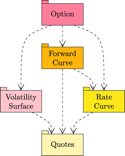
To cope with the various constraints of Section 5.1, our software architecture is composed of a Quotes module, a Rate Curve module, a Volatility Surface module, a Forward Curve module and an Option module, as shown in the UML package diagram of Figure 15.

Figure 15. Architecture UML package diagram.

Those modules contain the implementation of self-contained nodes from the domain model that encapsulate their local partial derivatives computation, as explained in Section 4.1.2.

All nodes provide their local partial derivatives very efficiently, taking advantage of local symbolic differentiation through implicit function theorem, mathematical simplifications and local computation reuses, as described in Section 4.2.2.

5.4. Results

A DerivativesController is instantiated and filled with the first- and second-order Greeks creation criteria of Table 1. Then the option premium and Greeks computation is triggered.

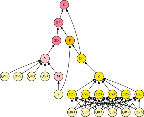
The corresponding runtime high-level domain model computational DAG is represented in Figure 16 where the 25 nodes are colored according to the module to which they belong.

Figure 16. Runtime global computational DAG.

The topological ordering traversal of the computational DAG is seeded on the source nodes from the Quotes module that are initialized with market quotes. It crosses all module boundaries and terminates on the C node from the Option module giving a 7.270 premium. It is displayed with the local results of each node (values and local partial derivatives) in Table 2.

Table 2. Node local results in topological ordering

The MCRE composes the 94 local partial derivatives computed by the nodes into the 82 Greeks in Table 3 (with values not requested to the DerivativesController labeled as “n.r.”).

Table 3. Computed greeks

5.5. Performance

The performance measurements were run on a Linux (4.4.0-53-generic x86_64) PC equipped with an Intel Core i7-6700 processor (4 cores, 3.8 GHz), 32 GB RAM, running Java 1.8.0_111.

The standard run was an evaluation of 2000 options.

To separately measure the premiums, local partial derivatives and total derivatives computation times, the runs were launched in four contexts:

(1)	Only computing the option premiums.
(2)	Computing the option premiums and the 94 local partial derivatives of all the nodes in the computational DAGs.
(3)	Computing the option premiums, the 94 local partial derivatives and the 82 requested first- and second-order total derivatives.
(4)	Computing the option premiums, the 94 local partial derivatives and the 82 total derivatives in parallel mode as described in Section 4.3.1.

The retained measures for each context are the averages on 20 standard runs.

Table 4. Time to price 2000 options

Context	Time	Ratio
Premiums	118 ms	$(1.0\times )$
Premiums + Local partial derivatives	206 ms	$(1.7\times )$
Premiums + Local partial derivatives + Total derivatives	308 ms	$(2.7\times )$
Premiums + Local partial derivatives + Total derivatives (in parallel mode)	262 ms	$(2.2\times )$

We can draw several interesting conclusions from the timings in Table 4.

First, the 94 local partial derivatives of all the nodes in the computational DAGs were computed with a ratio of 1:1.7 to the premiums-only computation time, i.e. only increasing the computation time by 70%. This result illustrates the unrivalled speed of local symbolic differentiation described in Section 4.2.2.

Second, the 82 requested first- and second-order total derivatives were computed with a ratio of 1:2.7 to the premiums-only computation time. This represents an overhead of 50% with respect to the computation time of the premiums and local partial derivatives. It illustrates CGAD efficiency, that comes from three factors:

(1)	working on coarse-grained computational DAGs.
(2)	exploiting total derivatives sparsity, as described in Section 4.3.2.
(3)	implementing lazy initialization on total derivatives, as described in Section 4.3.3.

Finally, if the MCRE runs in a dedicated separated thread, as introduced in Section 4.3.1, 50% of its overhead can be masked. This yields to a computation of the 82 requested first- and second-order total derivatives with a time ratio of 1:2.2 to the premiums-only computation time.

As a comparison, a finite difference engine would roughly exhibit a quadratic ratio of 1:56 on the same example. Indeed, it would require 1 evaluation for the premiums, 14 for the 14 first order Greeks and 41 for the 68 second order Greeks, exploiting symmetry.

In AD, the adjoint mode would compute the 14 first order Greeks of this example with a constant ratio around 1:3. However, the second order Greeks would require another AD pass on those 14 outputs, typically run in forward mode with a linear ratio around 1:1.5 $\times$ 14. The AD global ratio for the first- and second-order Greeks would therefore be linear and around 1 : 63. So, on this example, our CGAD implementation largely outperforms alternatives such as AD of finite difference.

6. Higher order

Faà di Bruno formula (1885) ensures that the joint-multivariate recursive definition of all total derivatives in a computational DAG exhibited in Formula (6) is not particular to first and second order, and can be extended to higher orders:

If a variable z depends on $n_z$ variables $y_1,\dots ,y_{n_z}$ and if all the up to mth order total derivatives of all the $y_i$ are known, it is possible to combine them with the up to mth order local partial derivatives of z to get all the up to mth order total derivatives of z.

The nodes in the computational DAGs just have to provide their local partial derivatives up to mth order and the MCRE has to be updated accordingly.

For instance at order 3, this yields Formula (8):(4) $$\begin{array}{cc}\hfill \forall (z,x,u,v)\in V^4,\frac{{\text{d}}^{3}z}{\text{d}x\text{d}u\text{d}v}& =\sum _{i=1}^{n_z}\sum _{j=1}^{n_z}\sum _{k=1}^{n_z}\frac{{\mathit{\partial }}^{3}z}{\mathit{\partial }{y}_i\mathit{\partial }{y}_j\mathit{\partial }{y}_k}·\frac{\text{d}{y}_i}{\text{d}x}·\frac{\text{d}{y}_j}{\text{d}u}·\frac{\text{d}{y}_k}{\text{d}v}\hfill \\ \hfill & +\sum _{i=1}^{n_z}\sum _{j=1}^{n_z}\frac{{\mathit{\partial }}^{2}z}{\mathit{\partial }{y}_i\mathit{\partial }{y}_j}·\left(\frac{{\text{d}}^2{y}_i}{\text{d}x\text{d}u}·\frac{\text{d}{y}_j}{\text{d}v}+\frac{{\text{d}}^2{y}_i}{\text{d}x\text{d}v}·\frac{\text{d}{y}_j}{\text{d}u}+\frac{{\text{d}}^2{y}_i}{\text{d}u\text{d}v}·\frac{\text{d}{y}_j}{\text{d}x}\right)\hfill \\ \hfill & +\sum _{i=1}^{n_z}\frac{\mathit{\partial }z}{\mathit{\partial }{y}_i}·\frac{{\text{d}}^3{y}_i}{\text{d}x\text{d}u\text{d}v}\hfill \\ \hfill \end{array}$$(4)

7. Conclusion

CGAD offers a new way to compute first- and second-order total derivatives that fully addresses software engineering concerns. It induces no coupling in software, letting all modules independently chose their local partial derivatives computation methods and connecting them using the multivariate chain rule. Additionally, its hybrid and flexible characteristics enables a cost-effective top-down integration.

Moreover, when combined with local symbolic differentiation, CGAD also addresses user experience concerns as it becomes exact up to machine precision, and runs significantly faster than AD and finite difference in certain contexts.

8. Disclaimer statement

The opinions and views expressed are those of the authors and do not necessarily represent those of Murex.

Additional information

Funding

The authors received no direct funding for this research.

Notes on contributors

Henri-Olivier Duché

Henri-Olivier Duché holds an engineering degree in computer science from CentraleSupélec. He has over 15 years of software development and quantitative finance experience. His current research activity is mainly focused on combining applied mathematics with software architecture and design principles.

François Galilée

François Galilée holds an engineering, PhD and post Doctorate degree in parallel computing. The main focus of his research is the design of efficient applications through parallel scheduling of its composing tasks by analysing the application’s data flow graph. Francois has over 25 years of software engineering experience on the design and operation of large scale distributed systems.

References

- Bauer, F. L. (1974). Computational graphs and rounding error. SIAM Journal on Numerical Analysis, 11(1), 87–96.
- Bischof, C. H., & Haghighat, M. R. (1996). Hierarchical approaches to automatic differentiation. Computational Differentiation: Techniques, Applications, and Tools, 83–94.
- Black, F. (1976). The pricing of commodity contracts. Journal of Financial Economics, 3(1--2), 167–179.
- Duché, H. O., & Galilée, F. (2017). Second order differentiation formula in a computational graph. Retrieved from https://ssrn.com/abstract=2905103
- Dijkstra, E. W. (1982). On the role of scientific thought. Selected writings on computing: a personal perspective. Springer. (pp. 60–66).
- Evans, E. (2004). Domain-driven design: Tackling complexity in the heart of software. Boston, MA: Addison-Wesley Professional.
- Francesco Faà di Bruno. (1885). Sullo sviluppo delle funzioni. Annali di scienze matematiche e fisiche, 6, 479.
- Fowler, M. (2002). Patterns of enterprise application architecture. Boston, MA: Addison-Wesley Longman Publishing.
- Gamma, E., Helm, R., Johnson, R., & Vlissides, J. (1995). Design patterns: Elements of reusable object-oriented software. Inc, Boston, MA: Addison-Wesley Longman Publishing.
- Gendler, D., Naumann, U., & Christianson, B. (2007). Automatic differentiation of assembler code. Proceedings of the IADIS International Conference on Applied Computing, 431–436.
- Giles, M., & Glasserman, P. (2006). Smoking adjoints: Fast monte carlo greeks. Risk, 19(1), 88–92.
- Griewank, A., & Walther, A. (2008). Evaluating derivatives: Principles and techniques of algorithmic differentiation. ( Number 105 in Other Titles in Applied Mathematics, 2nd ed.). Philadelphia, PA: SIAM.
- Henrard, M. (2011). Adjoint algorithmic differentiation: Calibration and implicit function theorem. OpenGamma Quantitative Research, (1).
- Henrard, M. (2011). Algorithmic differentiation in finance explained. Cham: Springer.
- Kaplan, W. (1952). Advanced calculus. Addison-Wesley mathematical series. Boston, MA: Addison-Wesley Press.
- Martin, R. C. (2008). Clean code: A handbook of agile software craftsmanship. Pearson Education
- Naumann, U. (2012). The art of differentiating computer programs: An introduction to algorithmic differentiation. Number 24 in Software, Environments, and Tools. Philadelphia, PA: SIAM.
- Sutter, H. (2005). Exceptional C++ style: 40 new engineering puzzles, programming problems, and solutions. Boston, MA: Addison-Wesley.