LQR-LMI control applied to convex-bounded domains

Abstract

Recently, propositions of new conditions necessary and sufficient in the controller’s synthesis, based on linear quadratic problems, have been especially combined with the mathematical description in the form of Linear Matrix Inequalities (LMI), expanding its applications for continuous and uncertain systems in convex-bounded domains. In this class of studies, the Linear Quadratic Regulator provides a good relationship between performance and eigenvalues allocation, based on minimization of energy signals of the state and control variables. Thus, this work permits to get less conservative conditions in LMI control through the use of parameter-dependent Lyapunov functions in obtaining robust controllers under a certain decay rate. Illustratively, application examples evaluate the performance of the proposed theorems, whose validation addresses tests of feasibility subject to variation limit of the decay rate and the analysis of the temporal behavior of the interest signals.

Keywords:

• linear quadratic regulator
• linear matrix inequalities
• decay rate
• parameter-dependent Lyapunov functions
• robust control

Public Interest Statement

Recently, control engineering has become essential in the industrial sector due to a competitive international market. However, an inefficient control system has a negative impact on the operation of these processes, whether for economic or security reasons. In this context, industrial plants have required robust controllers, in particular, to failures of power devices that receive the control signal and errors between the model and the real process. Thus, this paper aims to present matrices equations to design linear quadratic robust controllers, which allows to assign (a priori) a constraint at the oscillation level of sensed signals in the system. Therefore, the control engineers can lead a fine-tuning through design parameters. Finally, in a practical approach, our results provide control bounded signals and robustness for a 50% power drop in the back motor of a three degree of freedom helicopter.

1. Introduction

The theory of modern control involving the states feedback has advanced in recent years, in applications to electrical (Ollala, Levya, Aroudi, & Queineec, 2008, 2009), mechanical (Gritli & Belghith, 2017; Yue, An, & Sun, 2016), and chemical (Khairy, Elshafei, & Emara, 2010) nature systems, whose benefits are concentrated in the simplicity of implementation of real values instead of using poles and zeros. Of course, this fact considers that the variables chosen to compose the vector of states are available for sampling through appropriate sensors, or alternatively that they can be estimated.

Among the classes of control decisions, the indices based on quadratic functions stand out for presenting versatility as far as the performance, i.e. they use error or energy functions. In addition, it is possible to demonstrate a direct relationship between the second method of Lyapunov and the indices of quadratic performance in solving problems of optimal control, which consists of finding a rule through optimization (minimizing or maximizing) of a cost function, presenting restrictions in state and control variables that guarantee the asymptotic stability of the system in closed loop (Boyd, Ghaoui, Feron, & Balakrishnan, 1994).

In this context, the Linear Quadratic Regulator (LQR) corresponds to the extension of performance indices used in control techniques based in frequency domain, such as the Integral Square Error (ISE) and the Integral Absolute Error (IAE), to systems of multiple input and multiple outputs. Among the main characteristics of the optimal quadratic controller, it is highlighted: (1) the use of the model of representation in states space; (2) obtaining of the optimal control through the resolution of the Algebraic Riccati Equation (ARE); and (3) objective function with the weighting matrices $\mathcal{Q}$ and $\mathcal{R}$ in state and control vectors, respectively (Kumar, Raaja, & Jerome, 2016).

Among the various approaches to solving the ARE, the formulation by means of Linear Matrix Inequalities (LMI) has recently emerged as an efficient tool that introduces the use of matrices decision variables and convex constraints (Scherer & Weiland, 2005).

This mathematical description introduce facilities in searching for optimal solutions, in particular to problems of linear control, through computational packages available in free software, for example, the GNU Octave and Scilab (Pakshin, Emelianova, & Mazurov, 2012). Other related advantages, corresponds to: (1) structural failures (Assunção, Teixeira, Faria, Silva, & Cardim, 2007; Faria, Assunção, Teixeira, Cardim, & da Silva, 2009), guaranteeing robust stability and small oscillations in the occurrence of faults; (2) incorporation of performance indices (Corrêa & Freire, 2008; Hamada, 2016), which may be easily included by means of additional constraints through LMIs formulations (Chilali & Gahinet, 1996); however, it is noted that some studies evidence the incorporation of the decay rate to the original formulation in synthesis and analysis problems based on LMI (Xie, 2008); and (3) uncertainties (Boyd et al., 1994), which essentially studies some characteristics related to polytopic and norm-bounded uncertainties models. Notably, the polytopic class presents limited interest due to exponential growth in the number of vertices as the uncertainties increase. On the other hand, norm-bounded uncertainties (or, structured uncertainties), it is possible to exceed this limitation and to achieve less conservative conditions through the S-Procedure (Boyd et al., 1994). Furthermore, it is common to find bibliographic references that evaluate these uncertainty models in controller’s synthesis (de Souza & Trofino, 2010; Kothare, Balakrishnan, & Morari, 1996; Peres, Geromel, & Bernussou, 1993), just as it will be discussed in this work.

However, the formulations in matrices inequalities may present nonlinearities. In this case, it is important to apply classical methods that can linearize expressions, such as the Schur complement and/or exceed the limitations imposed by LMIs restrictions, through the application of the relaxation techniques that allow to reduce the conservatism assumption (Azizi, Torres, & Palhares, 2017; Lee, Park, Ji, & Won, 2007), such as Finsler Lemma and Reciprocal Projection Lemma. Consequently, there is an expanding of the search areas on convex optimization problems with reduces the controller’s norm and increases the computational complexity and feasibility (Buzachero, Assunção, Teixeira, & da Silva, 2012; da Silva, Assunção, Teixeira, Faria, & Buzachero, 2011). Thus, adding slack variables occurs the decoupling of the Lyapunov matrix in the state feedback matrix (Apkarian, Tuan, & Bernussou, 2001; Castelan, Tarbouriech, da Silva, & Queinnec, 2006), allowing the use of parameter-dependent Lyapunov functions in robust control.

As far as author’s knowledge, this paper has made the first attempt to reduce the LQR controller’s conservativeness for uncertain linear systems with polytopic and structured time-varying uncertainties, through a method based on parameter-dependent Lyapunov functions, guaranteeing the $\alpha$-stability.

The paper is organized as it follows. Section 2 presents a brief review about LQR controllers and uncertainty models. In Section 3, it is proposed the different forms of LQR-LMI controllers subject to decay rate applied to uncertain systems, whose cost function is obtained by output energy. Section 4 presents the development of less conservative conditions by Finsler Lemma applies to uncertain systems. In Section 5, it is presented the conditions by Reciprocal Projection Lemma only applied to polytopic model. Finally, Section 6 illustrates the validation of results through comparative analyzes in numerical applications, by means of a system mass-spring-damper, and practical implementation, considering the 3-DOF helicopter of Quanser, applied to case of actuators failures used as uncertain parameters.

Throughout the paper, $X\in {\mathfrak{R}}^{\mathit{nxn}}$ such as $X^{\prime }$ denotes its transpose, $X^{-1}$ its inverse, $X^{\perp }$ corresponds to a basis for a null space of X and $X>0(X\ge 0)$ means that X is positive (semi-) definite. It is considered that 0 and I denotes the matrix of elements null and identity matrix, respectively, with appropriate dimensions.

2. Preliminary concepts

Consider the linear time-invariant (LTI) system described by:(1) $$\begin{array}{c}\hfill \dot{x}(t)=Ax(t)+Bu(t)\end{array}$$(1)

where $x(t)\in {\mathfrak{R}}^n$ is the states vector and $u(t)\in {\mathfrak{R}}^m$ is the control input. The matrices A and B are real constants matrices of appropriate dimensions. Regarding the Equation (1), it will be presented below a review preliminary results and fundamental for the demonstration of proposed theorems.

2.1. Uncertainty model

The mathematical description of systems can cause uncertainty for different aspects, outlining errors between mathematical model and real system. In this context, the mathematical descriptions of these errors resulted in uncertainty representations, where the most important are the polytopic approaches, due to different operation points of the system, and the norm-bounded, based on prediction errors in identification processes (Bombois, 2000).

Therefore, to characterize these uncertainties, consider the system (1) and a pre-defined set in shape $[AB]\in \mathrm{\Omega }$, with the set $\mathrm{\Omega }$ describing the “uncertainty” in the matrices A and B. Thus, it is possible to constitute a polytopic system, through the set ${\mathrm{\Omega }}_P$, i.e.(2) $$\begin{array}{c}\hfill {\mathrm{\Omega }}_P=\text{Co}\left\{[A_1{B}_1],[A_2{B}_2],\dots ,[A_{\mathcal{N}}{B}_{\mathcal{N}}]\right\}\end{array}$$(2)

which corresponds to a convex set of $\mathcal{N}$ vertices. In this case, it is possible to notice that the vertices $[A_i{B}_i]$ of the polytope are obtained by combination of extreme values assumed by uncertain variables in the set $\left\{{\xi }_i:{\xi }_{i_{\mathit{min}}}<{\xi }_i<{\xi }_{i_{\mathit{max}}},i=1,\dots ,l\right\}$, with ${\xi }_i$ the time-varying parametric uncertainty and $\mathcal{N}=2^l$. In particular, this paper considers the parameter ${\xi }_i$ belonging to the unit simplex. On the other hand, the norm-bounded uncertainties are equivalent to:(3) $$\begin{array}{cc}\hfill \dot{x}(t)& =Ax(t)+Bu(t)+B_{p}p(t)\hfill \\ \hfill q(t)& =C_{q}x(t)+D_{q}u(t)\hfill \\ \hfill p(t)& =\mathrm{\Lambda }q(t)\hfill \end{array}$$(3)

where $\mathrm{\Lambda }:{\mathfrak{R}}_{+}\to {\mathfrak{R}}^{r\times r}$, q(t), $p(t)\in {\mathfrak{R}}^r$ are norm bounded time-varying uncertain matrix, regulated output and perturbation, respectively. The matrices $B_p$, $C_q$, and $D_q$ are real constants matrices of appropriate dimensions. It is possible to obtain useful variation, such as $||\mathrm{\Lambda }||\le 1$ or $||{\mathrm{\Lambda }}_i||\le 1$. However, the matrix constraint considered will be $||{\mathrm{\Lambda }}_i||\le 1$, i.e.(4) $$\begin{array}{c}\hfill \mathrm{\Lambda }=\left[\begin{array}{ccc}{\mathrm{\Lambda }}_1& \cdots & 0\\ ⋮& {\mathrm{\Lambda }}_i& ⋮\\ 0& \cdots & {\mathrm{\Lambda }}_r\end{array}\right]\end{array}$$(4)

Furthermore, to describe the norm-bounded uncertainties the set ${\mathrm{\Omega }}_N$ has the form,(5) $$\begin{array}{c}\hfill {\mathrm{\Omega }}_N=\left\{[A+B_p\mathrm{\Lambda }{C}_{q}B+B_p\mathrm{\Lambda }{D}_q]:||{\mathrm{\Lambda }}_i||\le 1,\mathrm{\Lambda }\text{diagonal}\right\}\end{array}$$(5)

It is observed that uncertainty region should contain the real system through a probability level, in which the uncertain parameters belong to the ellipsoid interior $(\epsilon )$ (Bombois, 2000),(6) $$\begin{array}{c}\hfill \epsilon =\left\{\lambda :{(\lambda -\widehat{\lambda })}^{\prime }{P}_{\lambda }^{-1}(\lambda -\widehat{\lambda })<\mathcal{X}\right\}\end{array}$$(6)

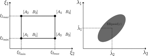
with $\lambda$ the uncertain parameters, $\widehat{\lambda }$ the estimated parameter, $P_{\lambda }$ the covariance matrix of $\widehat{\lambda }$ and $\mathcal{X}$ the desired level of probability. In some cases, it is possible to approximate the polytopic uncertainty in a norm-bounded uncertainty (Boyd et al., 1994); it reduces the number of LMIs lines, for example, in controller’s synthesis. Throughout, Figure 1 illustrates the uncertainties regions described previously in the case of two uncertainties applied in a system.

Figure 1. Uncertainty regions for polytopic and norm-bounded models, respectively.

2.2. Linear quadratic regulators

Consider the system (1). The problem LQR consists of finding a control law u(t) that minimizes a quadratic function $\mathcal{J}=f(x,u)$ such that (Kumar et al., 2016):(7) $$\begin{array}{c}\hfill \mathcal{J}\equiv {\int }_0^{\infty }(x{(t)}^{\prime }\mathcal{Q}x(t)+u{(t)}^{\prime }\mathcal{R}u(t))dt\end{array}$$(7)

where the weighting matrices $\mathcal{Q}={\mathcal{Q}}^{\prime }>0$ and $\mathcal{R}={\mathcal{R}}^{\prime }>0$ are known. In this problem, the control variables are expressed by a constant state feedback K, i.e.(8) $$\begin{array}{c}\hfill u(t)=-Kx(t)\end{array}$$(8)

Now, consider a quadratic Lyapunov function $V(x(t))=x{(t)}^{\prime }Px(t)$ to search a solution of the optimization problem,(9) $$\begin{array}{c}\hfill x{(t)}^{\prime }(\mathcal{Q}+K^{\prime }\mathcal{R}K)x(t)=-\frac{d(x{(t)}^{\prime }Px(t))}{\mathit{dt}}.\end{array}$$(9)

Therefore, the problem solution by minimizing of $\mathcal{J}$ (applied to deterministic systems), can be expressed by,(10) $$\begin{array}{c}\hfill u(t)=-Kx(t)=-{(\mathcal{R})}^{-1}{B}^{\prime }Px(t)\end{array}$$(10)

such that P satisfies the Riccati equation,(11) $$\begin{array}{c}\hfill A^{\prime }P+PA-PB{(\mathcal{R})}^{-1}{B}^{\prime }P+\mathcal{Q}=0\end{array}$$(11)

3. Linear quadratic regulator using linear matrix inequalities

In recent studies, there is a growing interest in linear quadratic problems, which have been widely combined to control theory, more specifically involving the synthesis of controllers by states feedback and the mathematical descriptions in terms of LMIs (Chancelier, Pakshin, & Soloviev, 2011; Dallali, Lee, Tsagarakis, & Caldwell, 2015; Fischer & Bhattacharya, 2009; Pandey, Mohanty ,Kishor, & Catalão, 2013; Priess, Conway, Choi, Popovich, & Radcliffe, 2015; Yang, Wu, & Chang, 2010). Thus, it will be proposed original formulations of robust LQR subject to decay rate, applied to convex-bounded domains.

3.1. Robust control

In general lines, the LQR control corresponds to a quadratic criterion that, by means of an optimization linear process, defines an optimal control law associated with energy functions of the state and control variables, seeking to balance the response speed of the system and the intensity of the control signal. This compromise between the energy functions allows defining the objective function,(12) $$\begin{array}{c}\hfill \mathcal{J}=\text{min}{\int }_0^{\infty }[x{(t)}^{\prime }\mathcal{Q}x(t)+u{(t)}^{\prime }\mathcal{R}u(t)]dt\end{array}$$(12)

It is observed that it is possible to obtain a preference relation among the values of the main diagonal elements of the matrix $\mathcal{R}$. Similarly, it is applied this concept of weighting for diagonal elements of the matrix $\mathcal{Q}$. Furthermore, it is possible to derive an upper bound for (12), as discussed in the next subsection, using the concept of maximum energy of the output.

3.2. Derivation of the upper bound using bounds on output energy

Consider the objective function (12). In Boyd et al. (1994), its possible to define the following relation,(13) $$\begin{array}{c}\hfill V(x)+{\int }_0^{\infty }x{(t)}^{\prime }(\mathcal{Q}+K^{\prime }\mathcal{R}K)x(t)dt<0.\end{array}$$(13)

Now, if the initial condition x(0) is known, an equivalent expression is,(14) $$\begin{array}{c}\hfill V(x(\infty ))-V(x(0))+{\int }_0^{\infty }x{(t)}^{\prime }(\mathcal{Q}+K^{\prime }\mathcal{R}K)x(t)dt<0.\end{array}$$(14)

Consider closed-loop system has all eigenvalues with real part negative, it has been $x(\infty )\to 0$, verified that,(15) $$\begin{array}{c}\hfill {\int }_0^{\infty }x{(t)}^{\prime }(\mathcal{Q}+K^{\prime }\mathcal{R}K)x(t)dt<V(x(0))=x{(0)}^{\prime }Px(0).\end{array}$$(15)

It is noted; however, there is a close relationship between the initial condition and Lyapunov function with respect to inequality (15). At this point, it is important to get equivalent expression in terms of LMIs, with upper bound equals the output energy, i.e.(16) $$\begin{array}{c}\hfill x{(0)}^{\prime }Px(0)\le \mu \end{array}$$(16)

Finally, using Schur complements and $W=P^{-1}$, it is implying,(17) $$\begin{array}{c}\hfill \left[\begin{array}{cc}\mu & \ast \\ x(0)& W\end{array}\right]\ge 0\end{array}$$(17)

where $\ast$ represents terms readily inferred from symmetry.

As an extension, we seek a polytope ${\mathrm{\Omega }}_C=\text{Co}\left\{x_1(0),x_2(0),\dots ,x_{\mathcal{P}}(0)\right\}$, whose maximum energy is at one of the vertices (Boyd et al., 1994). Therefore, we obtain the new upper bound on the output energy by the objective function,(18) $$\begin{array}{c}\hfill \left[\begin{array}{cc}\mu & \ast \\ x_i(0)& W\end{array}\right]\ge 0,i=1,\dots ,\mathcal{P}\end{array}$$(18)

3.3. Linear quadratic regulators with restriction of decay rate

In control systems, there is requirement to attend performance specifications that implies desired behavior of the output signals, i.e. the eigenvalues placement of closed-loop system. Such conditions may be easily included by means of additional constraints in the form of LMIs (Ollala et al., 2008). However, the disadvantage related to the process of eigenvalues placement is increased computational complexity. So, to reduce impacts on the computer processing, it is desirable to incorporate the decay rate in the original formulation of LMIs (Xie, 2008), i.e. we include the largest Lyapunov exponent in polytopic Linear Differential Inclusions (LDIs) (Ge, Chiu, & Wang, 2002) and norm-bound LDIs (Boyd et al., 1994), extended to LDI more general in terms of diagonal norm-bound, as proposed in the Theorems 3.1 and 3.2 of the following subsections. In fact, to the best of the author’s knowledge, LQR robust control design based on LMI with decay rate constraints is not well discussed in the literature.

3.3.1. Polytopic uncertainty

Theorem 3.1

The system (2) is stable by $u(t)=-Kx(t)$, using decay rate greater than or equal to $\alpha$ and guaranteed cost $\mathcal{J}$ inferior to $\mu$, if there exist matrices $W=W^{\prime }>0\in {\mathfrak{R}}^{n\times n}$ and $Z\in {\mathfrak{R}}^{m\times n}$, such that:$$\underset{\mu ,W,Z}{min}\mu$$

Subject   to(19) $$\begin{array}{c}\hfill \left[\begin{array}{ccc}{\mathcal{G}}_i& \ast & \ast \\ W& -{\mathcal{Q}}^{-1}& \ast \\ Z& 0& -{\mathcal{R}}^{-1}\end{array}\right]\le 0\end{array}$$(19) (20) $$\begin{array}{c}\hfill \left[\begin{array}{cc}\mu & \ast \\ x(0)& W\end{array}\right]\ge 0\end{array}$$(20)

where ${\mathcal{G}}_i=A_{i}W+W{A}_i^{\prime }+B_{i}Z+Z^{\prime }{B}_i^{\prime }+2\alpha W$. Therefore, state-feedback gain is $K=-Z{W}^{-1}$.

Multiplying every block (19) by ${\xi }_i\ge 0$, with $i=1$ to $i=\mathcal{N}$, results in,(21) $$\begin{array}{c}\hfill \left[\begin{array}{ccc}\mathcal{G}(\xi )& \ast & \ast \\ W& -{\mathcal{Q}}^{-1}& \ast \\ Z& 0& -{\mathcal{R}}^{-1}\end{array}\right]\le 0\end{array}$$(21)

where $\mathcal{G}(\xi )=({\sum }_{i=1}^{\mathcal{N}}{\xi }_i{A}_i)W+W{({\sum }_{i=1}^{\mathcal{N}}{\xi }_i{A}_i)}^{\prime }+({\sum }_{i=1}^{\mathcal{N}}{\xi }_i{B}_i)Z+Z^{\prime }{({\sum }_{i=1}^{\mathcal{N}}{\xi }_i{B}_i)}^{\prime }+2\alpha W$.

Using Schur complement, we obtain the equivalent LMI,(22) $$\begin{array}{c}\hfill A(\xi )W+WA{(\xi )}^{\prime }+B(\xi )Z+Z^{\prime }B{(\xi )}^{\prime }+2\alpha W+Z^{\prime }\mathcal{R}Z+W\mathcal{Q}W\le 0\end{array}$$(22)

Performing the change of variable $Z=-KW$ and multiplying the inequality (22) on the left and on the right by $W^{-1}=P$, and, after that, by $x{(t)}^{\prime }$ on the left and by x(t) on the right, can be found,(23) $$\begin{array}{c}\hfill x{(t)}^{\prime }P{A}_f(\xi )x(t)+x{(t)}^{\prime }{A}_f{(\xi )}^{\prime }Px(t)+2\alpha x{(t)}^{\prime }Px(t)\le -x{(t)}^{\prime }(K^{\prime }\mathcal{R}K+\mathcal{Q})x(t)\end{array}$$(23)

where $A_f(\xi )=(A(\xi )-B(\xi )K)$. Thus, considering the equation in state space systems, it is defined,(24) $$\begin{array}{c}\hfill \dot{V}(x)+2\alpha V(x)\le -x{(t)}^{\prime }(K^{\prime }\mathcal{R}K+\mathcal{Q})x(t)\end{array}$$(24)

or, simply,(25) $$\begin{array}{c}\hfill \dot{V}(x)+2\alpha V(x)\le 0,\alpha >0\end{array}$$(25)

Remark 1

In Equation (24), there was a change in the relation between Lyapunov inequality and guaranteed cost function. Consequently, the effect on inclusion of the term $2\alpha V(x)$ on inequality (13) motivates a re-evaluation of the expression given in (17). Thus, let V(x) be Lyapunov function (positive definite, by definition) and positive scalar $\alpha$. We can without loss of generality to assume the quadratic function $\mathcal{J}=f(x,u)$ as the upper bound for $-2\alpha V(x)-x{(t)}^{\prime }(K^{\prime }\mathcal{R}K+\mathcal{Q})x(t)$, i.e. it is possible to define a equivalent form such that $\dot{V}(x)\le -2\alpha V(x)-x{(t)}^{\prime }(K^{\prime }\mathcal{R}K+\mathcal{Q})x(t)\le -x{(t)}^{\prime }(K^{\prime }\mathcal{R}K+\mathcal{Q})x(t)$. Therefore, this condition is applies in all LMIs subject to decay rate that involve the upper bound for $\mathcal{J}$ in this work.

The proof of Theorem 3.1 is complete.

3.3.2. Norm-bounded uncertain

Theorem 3.2

The system (3) is stable by $u(t)=-Kx(t)$, using decay rate greater than or equal to $\alpha$ and guaranteed cost $\mathcal{J}$ inferior to $\mu$, if exists matrices $W=W^{\prime }>0\in {\mathfrak{R}}^{n\times n}$, $Z\in {\mathfrak{R}}^{m\times n}$ and $\mathrm{\Delta }\in {\mathfrak{R}}^{r\times r}$, such that:$$\underset{\mu ,W,Z,\mathrm{\Delta }}{min}\mu$$

Subject   to(26) $$\begin{array}{c}\hfill \left[\begin{array}{cccc}\mathrm{\Xi }& \ast & \ast & \ast \\ W& -{\mathcal{Q}}^{-1}& \ast & \ast \\ Z& 0& -{\mathcal{R}}^{-1}& \ast \\ C_{q}W+D_{q}Z& 0& 0& -\mathrm{\Delta }\end{array}\right]\le 0\end{array}$$(26) (27) $$\begin{array}{c}\hfill \left[\begin{array}{cc}\mu & \ast \\ x(0)& W\end{array}\right]\ge 0\end{array}$$(27)

with ${\delta }_1,\dots ,{\delta }_r>0$ such that:(28) $$\begin{array}{c}\hfill \mathrm{\Delta }=\left[\begin{array}{cccc}{\delta }_1& 0& \cdots & 0\\ 0& {\delta }_2& \cdots & 0\\ ⋮& ⋮& \ddots & ⋮\\ 0& 0& \cdots & {\delta }_r\end{array}\right]>0\end{array}$$(28)

where $\mathrm{\Xi }=W{A}^{\prime }+AW+Z^{\prime }{B}^{\prime }+BZ+2\alpha W+B_p\mathrm{\Delta }{B}_p^{\prime }$. Therefore, state-feedback gain is $K=-Z{W}^{-1}$.

Assuming $u(t)=-Kx(t)$ the feedback states gain, we can rewrite the equation of the states derived by,(29) $$\begin{array}{c}\hfill \dot{x}(t)=(A-BK)x(t)+B_{p}p(t)\end{array}$$(29)

In fact, imposing that $||{\mathrm{\Lambda }}_i||\le 1$, results in,(30) $$\begin{array}{c}\hfill p_i{(t)}^{\prime }{p}_i(t)\le q_i{(t)}^{\prime }{q}_i(t),i=1,\dots ,r\end{array}$$(30)

or,(31) $$\begin{array}{c}\hfill p_i^2(t)\le x{(t)}^{\prime }{(C_{q,i}-D_{q,i}K)}^{\prime }(C_{q,i}-D_{q,i}K)x(t)\end{array}$$(31)

where $C_{q,i}$ and $D_{q,i}$ to denote the ith row of $C_q$ and $D_q$, as well as $p_i(t)$ and $q_i(t)$ represent ith element of vectors p(t) e q(t).

Now, consider the closed-loop equation of the LQR controller subject to decay rate,(32) $$\begin{array}{c}\hfill \dot{x}{(t)}^{\prime }Px(t)+x{(t)}^{\prime }P\dot{x}(t)+2\alpha x{(t)}^{\prime }Px(t)\le -x{(t)}^{\prime }(\mathcal{Q}+K^{\prime }\mathcal{R}K)x(t).\end{array}$$(32)

However, considering the Equation (32) and applying the S-Procedure, it is possible to obtain (33). Then the inequality (34) it is obtain through the expansion of the operator sum, where the matrix variable to perform S-procedure $\widehat{\mathrm{\Delta }}$ implies in the existence of nonnegative ${\widehat{\delta }}_i$, i.e.(33) $$\begin{array}{cc}& \dot{x}{(t)}^{\prime }[P(A-BK)+{(A-BK)}^{\prime }P]x(t)+2x{(t)}^{\prime }P{B}_{p}p(t)+2\alpha x{(t)}^{\prime }Px(t)\hfill \\ \hfill & +\sum _{i=1}^r{\widehat{\delta }}_i\left(x{(t)}^{\prime }{(C_{q,i}-D_{q,i}K)}^{\prime }(C_{q,i}-D_{q,i}K)x(t)-p_i{(t)}^{\prime }{p}_i(t)\right)\hfill \\ \hfill & \le -x{(t)}^{\prime }(\mathcal{Q}+K^{\prime }\mathcal{R}K)x(t)\hfill \end{array}$$(33) (34) $$\begin{array}{cc}& x{(t)}^{\prime }{(A-BK)}^{\prime }Px(t)+p{(t)}^{\prime }{B}_p^{\prime }Px(t)+x{(t)}^{\prime }P(A-BK)x(t)\hfill \\ \hfill & +x{(t)}^{\prime }P{B}_{p}p(t)+2\alpha x{(t)}^{\prime }Px(t)-p{(t)}^{\prime }\widehat{\mathrm{\Delta }}p(t)\hfill \\ \hfill +x{(t)}^{\prime }(\mathcal{Q}+K^{\prime }\mathcal{R}K+{(C_q-D_{q}K)}^{\prime }\widehat{\mathrm{\Delta }}(C_q-D_{q}K))x(t)\le 0.\end{array}$$(34)

Finally, isolating the vector $[x{(t)}^{\prime }p{(t)}^{\prime }]$ on the left and the vector $\left[\begin{array}{c}x(t)\\ p(t)\end{array}\right]$ on the right, results in (35). Now, multiplying on the left by $\left[\begin{array}{cc}W& 0\\ 0& I\end{array}\right]$ and right by ${\left[\begin{array}{cc}W& 0\\ 0& I\end{array}\right]}^{\prime }$ the inequality (35), with $W=P^{-1}$, it is obtained the inequality (36).(35) $$\begin{array}{c}\hfill {\left[\begin{array}{c}x{(t)}^{\prime }\\ p{(t)}^{\prime }\end{array}\right]}^{\prime }\left[\begin{array}{cc}\left(\begin{array}{c}{(A-BK)}^{\prime }P+P(A-BK)+2\alpha P+\\ \mathcal{Q}+K^{\prime }\mathcal{R}K+{(C_q-D_{q}K)}^{\prime }\widehat{\mathrm{\Delta }}(C_q-D_{q}K)\end{array}\right)& \ast \\ B_p^{\prime }P& -\widehat{\mathrm{\Delta }}\end{array}\right]\left[\begin{array}{c}x(t)\\ p(t)\end{array}\right]\le 0\end{array}$$(35) (36) $$\begin{array}{c}\hfill \left[\begin{array}{cc}\left(\begin{array}{c}W{(A-BK)}^{\prime }+(A-BK)W+2\alpha W+W\mathcal{Q}W+\\ W{K}^{\prime }\mathcal{R}KW+W{(C_q-D_{q}K)}^{\prime }\widehat{\mathrm{\Delta }}(C_q-D_{q}K)W\end{array}\right)& \ast \\ B_p^{\prime }& -\widehat{\mathrm{\Delta }}\end{array}\right]\le 0.\end{array}$$(36)

Applying the Schur complement with the change of variables $\mathrm{\Delta }={\widehat{\mathrm{\Delta }}}^{-1}$ (described by Equation (28)) and $Z=-KW$, the inequality (36) is equivalent to,(37) $$\begin{array}{c}\hfill \left[\begin{array}{cccc}W{A}^{\prime }+AW+Z^{\prime }{B}^{\prime }+BZ+2\alpha W+B_p\mathrm{\Delta }{B}_p^{\prime }& \ast & \ast & \ast \\ W& -{\mathcal{Q}}^{-1}& \ast & \ast \\ Z& 0& -{\mathcal{R}}^{-1}& \ast \\ C_{q}W+D_{q}Z& 0& 0& -\mathrm{\Delta }\end{array}\right]\le 0.\end{array}$$(37)

The proof of Theorem 3.2 is complete. $\square$

4. Extended stability via Finsler Lemma

The use of relaxation techniques, in optimization problems with quadratic constraint, allows the expansion of the feasibility regions without to increase considerably the computational cost. Among the most widespread proposals, Finsler Lemma has been highlighted on applications of the continuous and discrete control theory, with interesting advantages in controller synthesis, for example, decoupling the Lyapunov matrix of states feedback gain (Castelan et al., 2006). This fact permits the use of less conservative functions, i.e. parameter-dependent Lyapunov functions (Buzachero et al., 2012). The consequence of this condition corresponds to increase of the feasibility regions in convex optimization problem, introducing a new (slack) matrices variable (de Oliveira & Skelton, 2001). Thus, in the following subsections, we propose the Theorems 4.1 and 4.2 that establish the lower bound on the decay rate of the LDIs in order to obtain less conservative original formulations of robust LQR-LMI. In addition, in the use of parameter-dependent Lyapunov functions for diagonal norm-bound LDIs, we considered the procedures adopted in Theorem 1 of Kunee and Banjerdpongchai (2008). To the author’s knowledge, these less conservative conditions of LQR robust design, obtained via Finsler Lemma, are not established in the literature.

4.1. Polytopic uncertain

Theorem 4.1

The system (2) is stable by $u(t)=-Kx(t)$, using decay rate greater than or equal to $\alpha$ and guaranteed cost $\mathcal{J}$ inferior to $\mu$, if for a given scalar $b>0$, exists matrices $Y\in {\mathfrak{R}}^{n\times n}$, $Z\in {\mathfrak{R}}^{m\times n}$ and ${\mathcal{W}}_i={\mathcal{W}}_i^{\prime }>0\in {\mathfrak{R}}^{n\times n}$, with $i=1,2,\dots ,\mathcal{N}$, such that:$$\underset{\mu ,{\mathcal{W}}_i,Z,Y}{min}\mu$$

Subject   to(38) $$\begin{array}{c}\hfill \left[\begin{array}{cccc}{A}_{i}Y+B_{i}Z+Y^{\prime }{A}_i^{\prime }+Z^{\prime }{B}_i^{\prime }+2\alpha {\mathcal{W}}_i& \ast & \ast & \ast \\ {\mathcal{W}}_i-Y^{\prime }+b{A}_{i}Y+b{B}_{i}Z& -bY-b{Y}^{\prime }& \ast & \ast \\ Y& 0& -{\mathcal{Q}}^{-1}& \ast \\ Z& 0& 0& -{\mathcal{R}}^{-1}\\ \end{array}\right]<0\end{array}$$(38) (39) $$\begin{array}{c}\hfill \left[\begin{array}{cc}\mu & \ast \\ x(0)& Y^{\prime }+Y-{\mathcal{W}}_i\end{array}\right]\ge 0\end{array}$$(39)

where $K=-Z{Y}^{-1}$.

Consider the simplex unit, ${\sum }_{i=1}^{\mathcal{N}}{\xi }_i=1,{\xi }_i\ge 0$. Multiplying every block (38) by ${\xi }_i\ge 0$, with $i=1$ to $i=\mathcal{N}$, results in (40).(40) $$\begin{array}{c}\hfill \left[\begin{array}{cccc}\left(\begin{array}{c}A(\xi )Y+Y^{\prime }A{(\xi )}^{\prime }+\\ B(\xi )Z+Z^{\prime }B{(\xi )}^{\prime }+2\alpha \mathcal{W}(\xi )\end{array}\right)& \ast & \ast & \ast \\ \mathcal{W}(\xi )-Y^{\prime }+bA(\xi )Y+bB(\xi )Z& -bY-b{Y}^{\prime }& \ast & \ast \\ Y& 0& -{\mathcal{Q}}^{-1}& \ast \\ Z& 0& 0& -{\mathcal{R}}^{-1}\end{array}\right]<0.\end{array}$$(40)

Let the variables, $w=\left[\begin{array}{c}x\\ \dot{x}\end{array}\right]$, $\mathcal{B}=[(A(\xi )-B(\xi )K)-I]$, ${\mathcal{B}}^{\perp }=\left[\begin{array}{c}I\\ (A(\xi )-B(\xi )K)\end{array}\right]$ and $\mathcal{L}=\left[\begin{array}{cc}2\alpha P(\xi )+K^{\prime }\mathcal{R}K+\mathcal{Q}& \ast \\ P(\xi )& 0\end{array}\right]$, with $P(\xi )=P{(\xi )}^{\prime }>0$. Thus, the development of conditions of the Finsler Lemma, results in:

(1)	If $\exists P(\xi )=P{(\xi )}^{\prime }>0$, such that $w^{\prime }\mathcal{L}w\le 0$ then, (41) $$\begin{array}{c}\hfill {\left[\begin{array}{c}x\\ \dot{x}\end{array}\right]}^{\prime }\left[\begin{array}{cc}2\alpha P(\xi )+K^{\prime }\mathcal{R}K+\mathcal{Q}& \ast \\ P(\xi )& 0\end{array}\right]\left[\begin{array}{c}x\\ \dot{x}\end{array}\right]\le 0\end{array}$$(41) and, expanding the vector multiplication, (42) $$\begin{array}{c}\hfill x^{\prime }P(\xi )\dot{x}+{\dot{x}}^{\prime }P(\xi )x+2\alpha x^{\prime }Px\le -x^{\prime }(K^{\prime }\mathcal{R}K+\mathcal{Q})x\end{array}$$(42) or, simply, (43) $$\begin{array}{c}\hfill x^{\prime }P(\xi )\dot{x}+{\dot{x}}^{\prime }P(\xi )x+2\alpha x^{\prime }Px\le 0.\end{array}$$(43) In addition, we consider the condition $\mathcal{B}w=0$, i.e. (44) $$\begin{array}{c}\hfill \left[\begin{array}{cc}(A(\xi )-B(\xi )K)& -I\end{array}\right]\left[\begin{array}{c}x\\ \dot{x}\end{array}\right]=0\end{array}$$(44) and, is equivalent to (45) $$\begin{array}{c}\hfill \dot{x}=(A(\xi )-B(\xi )K)x\end{array}$$(45)
(2)	If $\exists P(\xi )=P{(\xi )}^{\prime }>0$, such that, ${\mathcal{B}}^{{\perp }^{\prime }}\mathcal{L}{\mathcal{B}}^{\perp }$, then, (46) $$\begin{array}{c}\hfill {\left[\begin{array}{c}I\\ A(\xi )-B(\xi )K\end{array}\right]}^{\prime }\left[\begin{array}{cc}2\alpha P(\xi )+K^{\prime }\mathcal{R}K+\mathcal{Q}& \ast \\ P(\xi )& 0\end{array}\right]\left[\begin{array}{c}I\\ A(\xi )-B(\xi )K\end{array}\right]<0\end{array}$$(46) or, expanding, (47) $$\begin{array}{c}\hfill {(A(\xi )-B(\xi )K)}^{\prime }P+P(A(\xi )-B(\xi )K)+2\alpha P(\xi )\le -(K^{\prime }\mathcal{R}K+\mathcal{Q}).\end{array}$$(47) At this point, it is observed that the conditions 1 and 2 of the Finsler Lemma are satisfied, then the inequality (38) is obtained by:
(3)	If $\exists \mathcal{X}\in {\mathfrak{R}}^{2n\times n}$, $P(\xi )=P{(\xi )}^{\prime }>0$, then, (48) $$\begin{array}{c}\hfill \left[\begin{array}{cc}2\alpha P(\xi )+K^{\prime }\mathcal{R}K+\mathcal{Q}& \ast \\ P(\xi )& 0\end{array}\right]+\mathcal{X}\left[\begin{array}{cc}(A(\xi )-B(\xi )K)& -I\end{array}\right]+\\ \hfill \left[\begin{array}{c}{(A(\xi )-B(\xi )K)}^{\prime }\\ -I\end{array}\right]{\mathcal{X}}^{\prime }<0.\end{array}$$(48) Let us consider $\mathcal{X}=\left[\begin{array}{c}{X}_1\\ X_2\end{array}\right]$, such that, (49) $$\begin{array}{c}\hfill \left[\begin{array}{cc}2\alpha P(\xi )+K^{\prime }\mathcal{R}K+\mathcal{Q}& \ast \\ P(\xi )& 0\end{array}\right]+\left[\begin{array}{cc}{X}_1(A(\xi )-B(\xi )K)& -X_1\\ X_2(A(\xi )-B(\xi )K)& -X_2\end{array}\right]+\\ \hfill \left[\begin{array}{cc}{(A(\xi )-B(\xi )K)}^{\prime }{X}_1^{\prime }& {(A(\xi )-B(\xi )K)}^{\prime }{X}_2^{\prime }\\ -X_1^{\prime }& -X_2^{\prime }\end{array}\right]<0\end{array}$$(49) or, (50) $$\begin{array}{c}\hfill \left[\begin{array}{cc}\left(\begin{array}{c}{X}_1(A(\xi )-B(\xi )K)+{(A(\xi )-B(\xi )K)}^{\prime }{X}_1^{\prime }+\\ 2\alpha P(\xi )+K^{\prime }\mathcal{R}K+\mathcal{Q}\end{array}\right)& \ast \\ P(\xi )-X_1^{\prime }+X_2(A(\xi )-B(\xi )K)& -X_2-X_2^{\prime }\end{array}\right]<0.\end{array}$$(50) For an arbitrary choice of $X_1=M$ and $X_2=bM$, then, (51) $$\begin{array}{c}\hfill \left[\begin{array}{cc}\left(\begin{array}{c}M(A(\xi )-B(\xi )K)+{(A(\xi )-B(\xi )K)}^{\prime }{M}^{\prime }+\\ 2\alpha P(\xi )+K^{\prime }\mathcal{R}K+\mathcal{Q}\end{array}\right)& \ast \\ P(\xi )-M^{\prime }+bM(A(\xi )-B(\xi )K)& -bM-b{M}^{\prime }\end{array}\right]<0.\end{array}$$(51) Now, applying the congruence transformation $\left[\begin{array}{cc}{M}^{-1}& 0\\ 0& M^{-1}\end{array}\right]$ on the left and ${\left[\begin{array}{cc}{M}^{-1}& 0\\ 0& M^{-1}\end{array}\right]}^{\prime }$ on the right is found (52). Through the variables changes $Y={(M^{\prime })}^{-1}$ and $Z=-KY$, it is determined the inequality (53). (52) $$\begin{array}{c}\hfill \left[\begin{array}{cc}\left(\begin{array}{c}(A(\xi )-B(\xi )K){(M^{\prime })}^{-1}+\\ M^{-1}{(A(\xi )-B(\xi )K)}^{\prime }+2\alpha M^{-1}P(\xi ){(M^{\prime })}^{-1}+\\ M^{-1}{K}^{\prime }\mathcal{R}K{(M^{\prime })}^{-1}+M^{-1}\mathcal{Q}{(M^{\prime })}^{-1}\end{array}\right)& \ast \\ M^{-1}P(\xi ){(M^{\prime })}^{-1}-M^{-1}+b(A(\xi )-B(\xi )K){(M^{\prime })}^{-1}& -b{(M^{\prime })}^{-1}-b{M}^{-1}\end{array}\right]<0\end{array}$$(52) (53) $$\begin{array}{c}\hfill \left[\begin{array}{cc}\left(\begin{array}{c}A(\xi )Y+B(\xi )Z+Y^{\prime }A{(\xi )}^{\prime }+Z^{\prime }B{(\xi )}^{\prime }+\\ 2\alpha Y^{\prime }P(\xi )Y+Z^{\prime }\mathcal{R}Z+Y^{\prime }\mathcal{Q}Y\end{array}\right)& \ast \\ Y^{\prime }P(\xi )Y-Y^{\prime }+bA(\xi )Y+bB(\xi )Z& -bY-b{Y}^{\prime }\end{array}\right]<0.\end{array}$$(53) Since $\mathcal{W}(\xi )=Y^{\prime }P(\xi )Y$, implies that, (54) $$\begin{array}{c}\hfill \left[\begin{array}{cc}\left(\begin{array}{c}A(\xi )Y+B(\xi )Z+Y^{\prime }A{(\xi )}^{\prime }+Z^{\prime }B{(\xi )}^{\prime }+\\ 2\alpha \mathcal{W}(\xi )+Z^{\prime }\mathcal{R}Z+Y^{\prime }\mathcal{Q}Y\end{array}\right)& \ast \\ \mathcal{W}(\xi )-Y^{\prime }+bA(\xi )Y+bB(\xi )Z& -bY-b{Y}^{\prime }\end{array}\right]<0.\end{array}$$(54) Using Schur complement, in order to decompose the terms related to $\mathcal{R}$ and $\mathcal{Q}$, we obtain the equivalent LMI, (55) $$\begin{array}{c}\hfill \left[\begin{array}{cccc}\left(\begin{array}{c}A(\xi )Y+Y^{\prime }A{(\xi )}^{\prime }\\ +B(\xi )Z+Z^{\prime }B{(\xi )}^{\prime }+2\alpha \mathcal{W}(\xi )\end{array}\right)& \ast & \ast & \ast \\ \mathcal{W}(\xi )-Y^{\prime }+bA(\xi )Y+bB(\xi )Z& -bY-b{Y}^{\prime }& \ast & \ast \\ Y& 0& -{\mathcal{Q}}^{-1}& \ast \\ Z& 0& 0& -{\mathcal{R}}^{-1}\end{array}\right]<0\end{array}$$(55) where $Y\in {\mathfrak{R}}^{n\times n}$, $Y\ne Y^{\prime }$, $Z\in {\mathfrak{R}}^{m\times n}$, $\mathcal{W}(\xi )=Y^{\prime }P(\xi )Y$, $P(\xi )=P{(\xi )}^{\prime }>0$ and $K=-Z{Y}^{-1}$. Finally, the expansion of the uncertain matrices through its vertices results in (38).

The proof of Theorem 4.1 is complete.

Proposition 4.1

Consider the system (2). Given an initial condition x(0), positive definite matrices $\mathcal{Q}$ and $\mathcal{R}$, assume that exists matrices Y and Z, symmetric matrices ${\mathcal{W}}_i=\mathcal{W},\forall i=1,\dots ,\mathcal{N}$ and a positive scalar b such that (38) and (39) are feasible. Then, this result converges in the particular case using a quadratic Lyapunov functions.

Remark 2

It is verified, through practical tests, that as the parameter b becomes small enough, there is a increase of the feasibility region in controllers design obtained by Finsler Lemma (Geromel & Korogui, 2006). Thus, parameterized by the results presented in Geromel and Korogui (2006), it was decided to adopt the values of the millesimal order in practical applications, as it will be shown in Section 6 of this work.

4.2. Norm-bounded uncertain

Theorem 4.2

The system (3) is stable by $u(t)=-Kx(t)$, using decay rate greater than or equal to $\alpha$ and guaranteed cost $\mathcal{J}$ inferior to $\mu$, if for a given scalar $b>0$, exists matrices $Y\in {\mathfrak{R}}^{n\times n}$, $Z\in {\mathfrak{R}}^{m\times n}$, ${\mathrm{\Delta }}_i\in \mathfrak{R}$ and ${\mathcal{W}}_i={\mathcal{W}}_i^{\prime }>0\in {\mathfrak{R}}^{n\times n}$, with $i=1,2,\dots ,r$, such that:$$\underset{\mu ,{\mathcal{W}}_i,Z,Y,\mathrm{\Delta }}{min}\mu$$

Subject   to(56) $$\begin{array}{c}\hfill \left[\begin{array}{cc}AY+BZ+Y^{\prime }{A}^{\prime }+Z^{\prime }{B}^{\prime }+2\alpha {\mathcal{W}}_i+B_{p,i}{\mathrm{\Delta }}_i{B}_{p,i}^{\prime }\hfill & \ast \hfill \\ {\mathcal{W}}_i-Y^{\prime }+b(AY+BZ+B_{p,i}{\mathrm{\Delta }}_i{B}_{p,i}^{\prime })\hfill & b(b{B}_{p,i}{\mathrm{\Delta }}_i{B}_{p,i}^{\prime }-Y^{\prime }-Y)\hfill \\ Y\hfill & 0\hfill \\ Z\hfill & 0\hfill \\ C_{q,i}Y+D_{q,i}Z\hfill & 0\hfill \end{array}\right.\\ \hfill \left.\begin{array}{ccc}\ast \hfill & \ast \hfill & \ast \hfill \\ \ast \hfill & \ast \hfill & \ast \hfill \\ -{\mathcal{Q}}^{-1}\hfill & \ast \hfill & \ast \hfill \\ 0\hfill & -{\mathcal{R}}^{-1}\hfill & \ast \hfill \\ 0\hfill & 0\hfill & -{\mathrm{\Delta }}_i\hfill \end{array}\right]<0\end{array}$$(56) (57) $$\begin{array}{c}\hfill \left[\begin{array}{cc}\mu & \ast \\ x(0)& Y^{\prime }+Y-{\mathcal{W}}_i\end{array}\right]\ge 0\end{array}$$(57)

with,(58) $$\begin{array}{c}\hfill \mathrm{\Delta }=\left[\begin{array}{cccc}{\mathrm{\Delta }}_1& 0& \cdots & 0\\ 0& {\mathrm{\Delta }}_2& \cdots & 0\\ ⋮& ⋮& \ddots & ⋮\\ 0& 0& \cdots & {\mathrm{\Delta }}_r\end{array}\right]>0\end{array}$$(58)

where state feedback gain is reed as $K=-Z{Y}^{-1}$.

Consider the auxiliary variables from the Finsler Lemma:

$w=\left[\begin{array}{c}x\\ \dot{x}\\ p\end{array}\right]$, $\mathcal{B}=[(A-BK)-I{B}_p]$ and $\mathcal{L}=\left[\begin{array}{ccc}2\alpha P_i+K^{\prime }\mathcal{R}K+\mathcal{Q}& \ast & \ast \\ P_i& 0& \ast \\ 0& 0& 0\end{array}\right]$

If $\exists P_i=P_i^{\prime }>0$, such that, $w^{\prime }\mathcal{L}w\le 0$, then,(59) $$\begin{array}{c}\hfill {\left[\begin{array}{c}x\\ \dot{x}\\ p\end{array}\right]}^{\prime }\left[\begin{array}{ccc}2\alpha P_i+K^{\prime }\mathcal{R}K+\mathcal{Q}& \ast & \ast \\ P_i& 0& \ast \\ 0& 0& 0\end{array}\right]\left[\begin{array}{c}x\\ \dot{x}\\ p\end{array}\right]\le 0.\end{array}$$(59)

Now, considering the results of Kunee and Banjerdpongchai (2008) and using the S-Procedure to inequality (60), results in,(60) $$\begin{array}{c}\hfill \left[\begin{array}{ccc}2\alpha P_i+K^{\prime }\mathcal{R}K+\mathcal{Q}& \ast & \ast \\ P_i& 0& \ast \\ 0& 0& 0\end{array}\right]+\mathcal{X}\left[\begin{array}{ccc}(A-BK)& -I& B_{p,i}\end{array}\right]+\\ \hfill \left[\begin{array}{c}{(A-BK)}^{\prime }\\ -I\\ B_{p,i}^{\prime }\end{array}\right]{\mathcal{X}}^{\prime }+\left[\begin{array}{ccc}{(C_{q,i}-D_{q,i}K)}^{\prime }{\widehat{\mathrm{\Delta }}}_i(C_{q,i}-D_{q,i}K)& \ast & \ast \\ 0& 0& \ast \\ 0& 0& -{\widehat{\mathrm{\Delta }}}_i\end{array}\right]<0\end{array}$$(60)

where we have used $B_{p,i}$ to denote the ith column of $B_p$. Thus, with $\mathcal{X}=\left[\begin{array}{c}{X}_1\\ X_2\\ 0\end{array}\right]$, we have,(61) $$\begin{array}{c}\hfill \left[\begin{array}{ccc}2\alpha P_i+K^{\prime }\mathcal{R}K+\mathcal{Q}& \ast & \ast \\ P_i& 0& \ast \\ 0& 0& 0\end{array}\right]+\left[\begin{array}{c}{X}_1\\ X_2\\ 0\end{array}\right]\left[\begin{array}{ccc}(A-BK)& -I& B_{p,i}\end{array}\right]+\\ \hfill \left[\begin{array}{c}{(A-BK)}^{\prime }\\ -I\\ B_{p,i}^{\prime }\end{array}\right]{\left[\begin{array}{c}{X}_1\\ X_2\\ 0\end{array}\right]}^{\prime }+\left[\begin{array}{ccc}{(C_{q,i}-D_{q,i}K)}^{\prime }{\widehat{\mathrm{\Delta }}}_i(C_{q,i}-D_{q,i}K)& \ast & \ast \\ 0& 0& \ast \\ 0& 0& -{\widehat{\mathrm{\Delta }}}_i\end{array}\right]<0.\end{array}$$(61)

By a simple change of variables, $X_1=M$ and $X_2=bM$, we can obtain an equivalent LMI,(62) $$\begin{array}{c}\hfill \left[\begin{array}{ccc}2\alpha P_i+K^{\prime }\mathcal{R}K+\mathcal{Q}+{(C_{q,i}-D_{q,i}K)}^{\prime }{\widehat{\mathrm{\Delta }}}_i(C_{q,i}-D_{q,i}K)& \ast & \ast \\ P_i& 0& \ast \\ 0& 0& -{\widehat{\mathrm{\Delta }}}_i\end{array}\right]+\\ \hfill \left[\begin{array}{c}M\\ bM\\ 0\end{array}\right]\left[\begin{array}{ccc}(A-BK)& -I& B_{p,i}\end{array}\right]+\left[\begin{array}{c}{(A-BK)}^{\prime }\\ -I\\ B_{p,i}^{\prime }\end{array}\right]{\left[\begin{array}{c}M\\ bM\\ 0\end{array}\right]}^{\prime }<0\end{array}$$(62)

or,(63) $$\begin{array}{c}\hfill \left[\begin{array}{ccc}\left(\begin{array}{c}M(A-BK)+{(A-BK)}^{\prime }{M}^{\prime }+2\alpha P_i+K^{\prime }\mathcal{R}K+\\ \mathcal{Q}+{(C_{q,i}-D_{q,i}K)}^{\prime }{\widehat{\mathrm{\Delta }}}_i(C_{q,i}-D_{q,i}K)\end{array}\right)& \ast & \ast \\ bM(A-BK)-M^{\prime }+P_i& -b{M}^{\prime }-bM& \ast \\ B_{p,i}^{\prime }{M}^{\prime }& b{B}_{p,i}^{\prime }{M}^{\prime }& -{\widehat{\mathrm{\Delta }}}_i\end{array}\right]<0.\end{array}$$(63)

Now, pre-multiplying by $\left[\begin{array}{ccc}{M}^{-1}& 0& 0\\ 0& M^{-1}& 0\\ 0& 0& M^{-1}\end{array}\right]$ and post-multiplying by ${\left[\begin{array}{ccc}{M}^{-1}& 0& 0\\ 0& M^{-1}& 0\\ 0& 0& M^{-1}\end{array}\right]}^{\prime }$ the inequality (64), it is yield,$$\begin{array}{c}\hfill \left[\begin{array}{c}\left(\begin{array}{c}(A-BK){(M^{\prime })}^{-1}+M^{-1}{(A-BK)}^{\prime }+2\alpha M^{-1}{P}_i{(M^{\prime })}^{-1}+\\ M^{-1}{K}^{\prime }\mathcal{R}K{(M^{\prime })}^{-1}+M^{-1}\mathcal{Q}{(M^{\prime })}^{-1}+\\ M^{-1}{(C_{q,i}-D_{q,i}K)}^{\prime }{\widehat{\mathrm{\Delta }}}_i(C_{q,i}-D_{q,i}K){(M^{\prime })}^{-1}\end{array}\right)\\ b(A-BK){(M^{\prime })}^{-1}-M^{-1}+M^{-1}{P}_i{(M^{\prime })}^{-1}\\ M^{-1}{B}_{p,i}^{\prime }\end{array}\right.\end{array}$$ (64) $$\begin{array}{c}\hfill \left.\begin{array}{cc}\ast & \ast \\ -b{M}^{-1}-b{(M^{\prime })}^{-1}& \ast \\ b{M}^{-1}{B}_{p,i}^{\prime }& -M^{-1}{\widehat{\mathrm{\Delta }}}_i{(M^{\prime })}^{-1}\end{array}\right]<0\end{array}$$(64)

Let $Y={(M^{\prime })}^{-1}$, then,(65) $$\begin{array}{c}\hfill \left[\begin{array}{ccc}\left(\begin{array}{c}(A-BK)Y+Y^{\prime }{(A-BK)}^{\prime }+2\alpha Y^{\prime }{P}_{i}Y+\\ Y^{\prime }{K}^{\prime }\mathcal{R}KY+Y^{\prime }\mathcal{Q}Y+\\ Y^{\prime }{(C_{q,i}-D_{q,i}K)}^{\prime }{\widehat{\mathrm{\Delta }}}_i(C_{q,i}-D_{q,i}K)Y\end{array}\right)& \ast & \ast \\ b(A-BK)Y-Y^{\prime }+Y^{\prime }{P}_{i}Y& -b{Y}^{\prime }-bY& \ast \\ Y^{\prime }{B}_{p,i}^{\prime }& b{Y}^{\prime }{B}_{p,i}^{\prime }& -Y^{\prime }{\widehat{\mathrm{\Delta }}}_{i}Y\end{array}\right]<0\end{array}$$(65)

and, through of the change of variable ${\mathcal{W}}_i=Y^{\prime }{P}_{i}Y$,(66) $$\begin{array}{c}\hfill \left[\begin{array}{ccc}\left(\begin{array}{c}(A-BK)Y+Y^{\prime }{(A-BK)}^{\prime }+2\alpha {\mathcal{W}}_i+\\ Y^{\prime }{K}^{\prime }\mathcal{R}KY+Y^{\prime }\mathcal{Q}Y+\\ Y^{\prime }{(C_{q,i}-D_{q,i}K)}^{\prime }{\widehat{\mathrm{\Delta }}}_i(C_{q,i}-D_{q,i}K)Y\end{array}\right)& \ast & \ast \\ b(A-BK)Y-Y^{\prime }+{\mathcal{W}}_i& -b{Y}^{\prime }-bY& \ast \\ Y^{\prime }{B}_{p,i}^{\prime }& b{Y}^{\prime }{B}_{p,i}^{\prime }& -Y^{\prime }{\widehat{\mathrm{\Delta }}}_{i}Y\end{array}\right]<0\end{array}$$(66)

Now, applying the congruence transformation $\left[\begin{array}{ccc}I& 0& 0\\ 0& I& 0\\ 0& 0& {(Y^{\prime })}^{-1}\end{array}\right]$ on the left and ${\left[\begin{array}{ccc}I& 0& 0\\ 0& I& 0\\ 0& 0& {(Y^{\prime })}^{-1}\end{array}\right]}^{\prime }$ on the right is found (67).(67) $$\begin{array}{c}\hfill \left[\begin{array}{ccc}\left(\begin{array}{c}(A-BK)Y+Y^{\prime }{(A-BK)}^{\prime }+2\alpha {\mathcal{W}}_i+\\ Y^{\prime }{K}^{\prime }\mathcal{R}KY+Y^{\prime }\mathcal{Q}Y+\\ Y^{\prime }{(C_{q,i}-D_{q,i}K)}^{\prime }{\widehat{\mathrm{\Delta }}}_i(C_{q,i}-D_{q,i}K)Y\end{array}\right)& \ast & \ast \\ b(A-BK)Y-Y^{\prime }+{\mathcal{W}}_i& -b{Y}^{\prime }-bY& \ast \\ B_{p,i}^{\prime }& b{B}_{p,i}^{\prime }& -{\widehat{\mathrm{\Delta }}}_i\end{array}\right]<0\end{array}$$(67)

In order to eliminate the nonlinearities, it is applied the Schur complement with the change of variables $Z=-KY$ and ${\mathrm{\Delta }}_i={\widehat{\mathrm{\Delta }}}_i^{-1}$, such that (56) is obtained.

The proof of Theorem 4.2 is complete.

Proposition 4.2

Consider the system (3). Given an initial condition x(0), positive definite matrices $\mathcal{Q}$ and $\mathcal{R}$, assume that exists matrices Y, Z and $\mathrm{\Delta }$, symmetric matrices ${\mathcal{W}}_i=\mathcal{W},\forall i=1,\dots ,r$ and a positive scalar b such that (56)–(58) are feasible. Then, this result converges in the particular case using a quadratic Lyapunov functions.

4.3. Derivation of the upper bound

This subsection is dedicated to demonstrate the extension to upper bound via Finsler Lemma, i.e.(68) $$\begin{array}{c}\hfill \left[\begin{array}{cc}\mu & \ast \\ x(0)& Y^{\prime }+Y-{\mathcal{W}}_i\end{array}\right]\ge 0.\end{array}$$(68)

In this case, for the sufficiency proof, it will be considered the results of Daafouz and Bernussou (2001), such that (68) is feasible and, therefore, $Y^{\prime }+Y-{\mathcal{W}}_i\ge 0$. So, given Y (full rank) and ${\mathcal{W}}_i$ (strictly positive definite), we have,(69) $$\begin{array}{c}\hfill ({\mathcal{W}}_i-Y){\mathcal{W}}_i^{-1}{({\mathcal{W}}_i-Y)}^{\prime }\ge 0\end{array}$$(69)

or, equivalently, $Y{\mathcal{W}}_i^{-1}{Y}^{\prime }\ge Y^{\prime }+Y-{\mathcal{W}}_i$. Thus, the equivalent LMI is,(70) $$\begin{array}{c}\hfill \left[\begin{array}{cc}\mu & \ast \\ x(0)& Y{\mathcal{W}}_i^{-1}{Y}^{\prime }\end{array}\right]\ge 0\end{array}$$(70)

Now, decomposing the terms $\left[\begin{array}{cc}I& 0\\ 0& Y\end{array}\right]$ on the left and ${\left[\begin{array}{cc}I& 0\\ 0& Y\end{array}\right]}^{\prime }$ on the right, results in,(71) $$\begin{array}{c}\hfill \left[\begin{array}{cc}I& 0\\ 0& Y\end{array}\right]\left[\begin{array}{cc}\mu & \ast \\ Y^{-1}x(0)& {\mathcal{W}}_i^{-1}\end{array}\right]{\left[\begin{array}{cc}I& 0\\ 0& Y\end{array}\right]}^{\prime }\ge 0.\end{array}$$(71)

In order to apply the complement of Schur, we show that,(72) $$\begin{array}{c}\hfill x{(0)}^{\prime }{(Y^{\prime })}^{-1}{\mathcal{W}}_i{Y}^{-1}x(0)\le \mu \end{array}$$(72)

and, with the change of variable, ${\mathcal{W}}_i=Y^{\prime }{P}_{i}Y$, yields the LMI condition:(73) $$\begin{array}{c}\hfill x{(0)}^{\prime }{(Y^{\prime })}^{-1}{Y}^{\prime }{P}_{i}Y{Y}^{-1}x(0)\le \mu .\end{array}$$(73)

Finally, consider the simplex unit, ${\sum }_{i=1}^r{\xi }_i=1,{\xi }_i\ge 0$. Multiplying (73) by ${\xi }_i$, with $i=1$ to $i=r$, results in $x{(0)}^{\prime }P(\mathrm{\Delta })x(0)\le \mu$.

Remark 3

It is observed, in this case, that the only procedure variation involves the limits of variable i, where in the model of polytopic uncertainty it is considered the number of vertices and the model of bounded-norm uncertainty by the number of uncertain parameters.

5. Extended stability via reciprocal projection lemma

In this subsection, it is proposed through the Theorem 5.1 new LMI-based LQR design via Reciprocal Projection Lemma (Apkarian et al., 2001). Here, we consider the polytope described by the vertices in the form of $\text{Co}\left\{[A_1{B}_1{x}_1(0)],\dots ,[A_{\mathcal{N}+\mathcal{P}}{B}_{\mathcal{N}+\mathcal{P}}{x}_{\mathcal{N}+\mathcal{P}}(0)]\right\}$. Lastly, we get less conservative conditions subject to decay rate without the use of additional LMIs lines.

Theorem 5.1

The system (2) is stable by $u(t)=-Kx(t)$, using decay rate greater than or equal to $\alpha$ and guaranteed cost $\mathcal{J}$ inferior to $\mu$, if there exist matrices $V\in {\mathfrak{R}}^{n\times n}$, $Z\in {\mathfrak{R}}^{m\times n}$ and $X_i=X_i^{\prime }>0\in {\mathfrak{R}}^{n\times n}$, such that:$$\underset{\mu ,X_i,Z,Y}{min}\mu$$

Subject   to(74) $$\begin{array}{c}\hfill \left[\begin{array}{ccccc}-(V^{\prime }+V)& \ast & \ast & \ast & \ast \\ A_{i}V+B_{i}Z+\alpha V+X_i& -X_i& \ast & \ast & \ast \\ V& 0& -X_i& \ast & \ast \\ V& 0& 0& -{\mathcal{Q}}^{-1}& \ast \\ Z& 0& 0& 0& -{\mathcal{R}}^{-1}\end{array}\right]<0\end{array}$$(74) (75) $$\begin{array}{c}\hfill \left[\begin{array}{cc}\mu & \ast \\ x_i(0)& X_i\end{array}\right]\ge 0\end{array}$$(75)

with $i=1,\dots ,\mathcal{N}+\mathcal{P}$. Thus, the state feedback gain is recovered as $K=-Z{V}^{-1}$.

Consider the Riccati equation subject to decay rate and, initially, a Lyapunov inequality on P, such that:(76) $$\begin{array}{c}\hfill P(A-BK)+{(A-BK)}^{\prime }P+2\alpha P+K^{\prime }\mathcal{R}K+\mathcal{Q}\le 0.\end{array}$$(76)

Assume that $\mathrm{\Psi }=K^{\prime }\mathcal{R}K+\mathcal{Q}$, $S=P(A-BK)+\alpha P$ and $S^{\prime }={(A-BK)}^{\prime }P+\alpha P$. Thus, consider the condition (2) from the Reciprocal Projection Lemma, such that,(77) $$\begin{array}{c}\hfill \left[\begin{array}{cc}{K}^{\prime }\mathcal{R}K+\mathcal{Q}+T-(W+W^{\prime })& \ast \\ P(A-BK)+\alpha P+W& -T\end{array}\right]<0.\end{array}$$(77)

Applying the congruence transformation $\left[\begin{array}{cc}{(W^{\prime })}^{-1}& 0\\ 0& P^{-1}\end{array}\right]$ on the left and ${\left[\begin{array}{cc}{(W^{\prime })}^{-1}& 0\\ 0& P^{-1}\end{array}\right]}^{\prime }$ on the right, is found (78).(78) $$\begin{array}{c}\hfill \left[\begin{array}{cc}\left(\begin{array}{c}{(W^{\prime })}^{-1}{K}^{\prime }\mathcal{R}K{W}^{-1}+{(W^{\prime })}^{-1}\mathcal{Q}{W}^{-1}+\\ {(W^{\prime })}^{-1}T{W}^{-1}-({(W^{\prime })}^{-1}+W^{-1})\end{array}\right)& \ast \\ (A-BK)W^{-1}+\alpha W^{-1}+P^{-1}& -P^{-1}T{P}^{-1}\end{array}\right]<0\end{array}$$(78)

Defining the variables, $X=P^{-1}$ and $V=W^{-1}$, we can express (78) as follows,(79) $$\begin{array}{c}\hfill \left[\begin{array}{cc}{V}^{\prime }{K}^{\prime }\mathcal{R}KV+V^{\prime }\mathcal{Q}V+V^{\prime }TV-(V^{\prime }+V)& \ast \\ (A-BK)V+\alpha V+X& -XTX\end{array}\right]<0.\end{array}$$(79)

Now, proceeding a new change of variables $T=X^{-1}$ and $Z=-KV$, results in,(80) $$\begin{array}{c}\hfill \left[\begin{array}{cc}{Z}^{\prime }\mathcal{R}Z+V^{\prime }\mathcal{Q}V+V^{\prime }{X}^{-1}V-(V^{\prime }+V)& \ast \\ AV+BZ+\alpha V+X& -X\end{array}\right]<0.\end{array}$$(80)

By application of the Schur complement, decomposing the quadratic terms, yields,(81) $$\begin{array}{c}\hfill \left[\begin{array}{ccccc}-(V^{\prime }+V)& \ast & \ast & \ast & \ast \\ AV+BZ+\alpha V+X& -X& \ast & \ast & \ast \\ V& 0& -X& \ast & \ast \\ V& 0& 0& -{\mathcal{Q}}^{-1}& \ast \\ Z& 0& 0& 0& -{\mathcal{R}}^{-1}\end{array}\right]<0\end{array}$$(81)

and, expanding the inequality (81) in terms of polytope vertices, it is given by,(82) $$\begin{array}{c}\hfill \left[\begin{array}{ccccc}-(V^{\prime }+V)& \ast & \ast & \ast & \ast \\ A_{i}V+B_{i}Z+\alpha V+X_i& -X_i& \ast & \ast & \ast \\ V& 0& -X_i& \ast & \ast \\ V& 0& 0& -{\mathcal{Q}}^{-1}& \ast \\ Z& 0& 0& 0& -{\mathcal{R}}^{-1}\end{array}\right]<0.\end{array}$$(82)

Finally, consider the simplex unit, ${\sum }_{i=1}^{\mathcal{N}+\mathcal{P}}{\xi }_i=1,{\xi }_i\ge 0$. Multiplying (82) by ${\xi }_i\ge 0$, the inequality (83) is obtained.(83) $$\begin{array}{c}\hfill \left[\begin{array}{ccccc}-(V^{\prime }+V)& \ast & \ast & \ast & \ast \\ A(\xi )V+B(\xi )Z+\alpha V+X(\xi )& -X(\xi )& \ast & \ast & \ast \\ V& 0& -X(\xi )& \ast & \ast \\ V& 0& 0& -{\mathcal{Q}}^{-1}& \ast \\ Z& 0& 0& 0& -{\mathcal{R}}^{-1}\end{array}\right]<0.\end{array}$$(83)

The proof of the inequality (75) is found in Section (3.2), assuming in (18) the $\mathcal{N}+\mathcal{P}$ vertices of the polytope.

The proof of Theorem 5.1 is complete.

Remark 4

Clearly, the design methodologies proposed in this work are conducted in off-line. However, problems of industrial scale need to be mitigated quickly, either for economic reasons or for reasons of safety in the operation of processes. In this case, LQR control has beem used in industrial applications of control engineering (continuous stirred tank reactor, for example) to design Proportional-Integral-Derivative (PID) controllers (Ge et al., 2002). Furthermore, the computational effort to search solutions in control varies with the uncertainty and the dimensions of the plant model. A drawback refers to severe delays in the implementation of a controller that attend the new design conditions. These facts motivate the application of techniques that provide real-time solutions with less complexity, and therefore, we aim to reduce the number of lines of LMIs to be programmed in control algorithms and to apply different kind of uncertainty models. It is also important to design such controllers to be robust to uncertainties of real process. However, from a control theory point of view, the use of one single Lyapunov function to define a state feedback control law leads to some conservativeness, seem in the Theorems 3.1 and 3.2. Thus, we consider techniques of relaxation matrices, discussed in Sections 4 and 5, that allowed to adopt parameter-dependent Lyapunov functions and has had advantages in terms of extended marginal stability, i.e. larger feasibility regions in terms of decay rate, which yields reduced magnitudes of the designed controllers (an important condition in practical implementations) besides to insure the robust stability of LDIs.

6. Numerical example and practical implementation

At this section, it will be submitted two applications to explain the advantages and disadvantages between models of uncertainties and relaxation techniques, based on theorems proposed in this work. It is informed that the computational package LMIlab and interface YALMIP (Löfberg, 2004), in MATLAB environment, were used to compute the solution of the optimization problem. As far as author’s knowledge, this paper has made the first attempt to apply uncertainty models in the case of extended stability in LQR-LMI control subject to decay rate, that considers an upper bound based on maximum energy of the output. Therefore, do not involve comparative analyzes with literature.

6.1. Practical application in the 3-DOF helicopter

Consider the schematic model of Figure 2 of the 3-DOF helicopter. Two DC motors are mounted at the ends of a rectangular frame and drive two propellers. The motors axis are parallel and the thrust vector is normal to the frame (Quanser, 2002).

Figure 2. Schematic drawing of 3-DOF helicopter (Quanser, 2002).

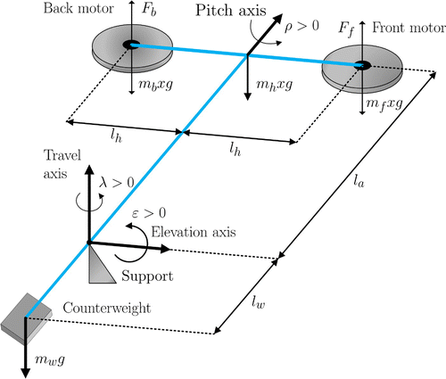
As described in Buzachero, Assunção, Teixeira, & da Silva (2012), the arm is gimbaled on a 2-DOF instrumented joint and it is free to pitch and yaw. The other end of the arm carries a counterweight which makes the effective mass light enough to enable the motors to raise the helicopter. A positive voltage applied on the front motor $(V_f)$ causes a positive pitch, while a positive voltage applied to the back motor $(V_b)$ causes a negative pitch (angle pitch $(\rho )$). A positive voltage to either motors causes an elevation of the whole body (angle elevation $(\epsilon )$ of the arm). If the body pitches, the impulsion vector results in the displacement of the system (angle travel $(\lambda )$ of the systems). The purpose of this experiment is to design a control system to track and regulate the elevation and travel of the 3-DOF helicopter. The trajectory of the helicopter was divided into three stages: (a) to elevate the helicopter $27.5^{\circ }$ reaching the yaw angle $\epsilon =0^{\circ }$; (b) the helicopter travels ${120}^{\circ }$, and (c) the helicopter performs the landing recovering the initial angle $(\epsilon =-27.5^{\circ }\approx -0.48$ rad).

In the state space model that describes the helicopter the state is x(t), the control is u(t) and A, B are defined by:$$\begin{array}{c}\hfill x(t)={[\epsilon \rho \lambda \dot{\epsilon }\dot{\rho }\dot{\lambda }\xi \gamma ]}^{\prime },u(t)=\left[\begin{array}{c}{V}_f\\ V_b\end{array}\right]\end{array}$$ $$\begin{array}{c}\hfill A=\left[\begin{array}{cccccccc}0& 0& 0& 1& 0& 0& 0& 0\\ 0& 0& 0& 0& 1& 0& 0& 0\\ 0& 0& 0& 0& 0& 1& 0& 0\\ 0& 0& 0& 0& 0& 0& 0& 0\\ 0& 0& 0& 0& 0& 0& 0& 0\\ 0& \frac{(2m_f{l}_a-m_w{l}_w)g}{2m_f{l}_a^2+2m_f{l}_h^2+2m_f{l}_w^2}& 0& 0& 0& 0& 0& 0\\ 1& 0& 0& 0& 0& 0& 0& 0\\ 0& 0& 1& 0& 0& 0& 0& 0\end{array}\right],\end{array}$$ $$\begin{array}{c}\hfill B=\left[\begin{array}{cc}0& 0\\ 0& 0\\ 0& 0\\ \frac{l_a{k}_f}{m_w{l}_w^2+2m_f{l}_a^2}& \frac{l_a{k}_f}{m_w{l}_w^2+2m_f{l}_a^2}\\ \frac{1}{2}\frac{k_f}{m_f{l}_h}& -\frac{1}{2}\frac{k_f}{m_f{l}_h}\\ 0& 0\\ 0& 0\\ 0& 0\end{array}\right].\end{array}$$

Remark 5

The state variables $\xi$ and $\gamma$ represent the integrals of the angles $\epsilon$ and $\lambda$, respectively, and occurs that the system does not reach the null values for these state variables. In addition, in Table 1 are described the constants that appear in the matrices A and B.

Now, to add uncertainty to the system, it was implemented a loss of $50\%$ of the power in back motor, by insertion a timer switch connected to an amplifier with a gain of 0.5 acting directly on engine. Thus, it was constituted a polytope of two vertices with an uncertainty in the input matrix of the system.

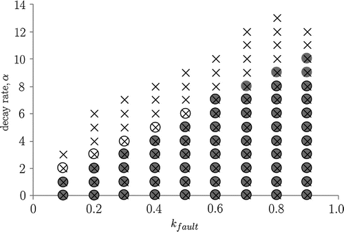
The performance analysis of the proposals, with polytopic uncertain, it was evaluated through the feasibility regions based on upper bounds obtained by Theorem 3.1 (quadratic stability), Theorem 4.1 (extended stability via Finsler Lemma), and Theorem 5.1 (extended stability via Reciprocal Projection Lemma). In this case, the graphic lists the parameter $\alpha$ (integer values) and the power loss (constant $k_{\mathit{fault}}$) described as a failure, where $k_{\mathit{fault}}=1.0$ correspond the case of no actuator failure. It was also adopted that $\mathcal{R}=0.025\times \text{diag}(1,1)$ and $\mathcal{Q}=\text{diag}(100,1,10,0.01,0.01,2,10,0.1)$.

Table 1. Helicopter parameters

Power constant of the propeller (found experimentally)	$k_f$	0.1188
Mass of the helicopter body (kg)	$m_h$	1.158
Mass of counterweight (kg)	$m_w$	1.87
Mass of the whole front of the propeller (kg)	$m_f$	$m_h/2$
Mass of the whole back of the propeller (kg)	$m_b$	$m_h/2$
Distance between each axis of pitch and motor (m)	$l_h$	0.1778
Distance between the lift axis and the body of the helicopter (m)	$l_a$	0.6604
Distance between the axis of elevation and the counterweight (m)	$l_w$	0.4699
Gravitational constant (m/${\text{s}}^2$)	g	9.81

In the graphic of Figure 3, the Theorem 5.1 presents difficulties to search feasibility solutions, especially for severe failures; however, it is noticed some improvements in relation to Theorem 3.1 for $k_{\mathit{fault}}>0.6$. Furthermore, the results obtained by Theorem 4.1 presents higher levels of feasibility, due to choose of the constant b, which contributes to decay rate increase. On the other hand, the solution associated with $k_{\mathit{fault}}=0.7$ and $\alpha =11$, derived from Theorem 4.1, was unfeasible. Thus, it was explored a nearness region to this condition, that is $\alpha =11.01$, which led to convergence of the algorithm, as expected.

Figure 3. Feasibility regions to polytopic uncertain ($\circ$: Theorem 3.1; $\times$: Theorem 4.1; grey color: Theorem 5.1).

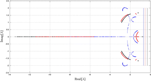
Furthermore, Figure 4 illustrates an analysis of the eigenvalues behavior of the uncertain closed-loop system, by varying the parameter $\xi$, partitioned in 125 values in (2), taking into account their $\alpha$-stability and the condition $||K||\approx 250$. Therefore, it is verified that the Theorem 5.1 further a significant spreading of eigenvalues in the complex plane, by restricting of the real part of the eigenvalues to values greater than $-8.5283$, this implies directly in reduced norm of K. In contrast, we have the value $-11.4199$ by Theorem 4.1 and $-13,4860$ by Theorem 3.1.

Figure 4. Eigenvalues behavior of the uncertain closed-loop system (black color: Theorem 3.1; red color: Theorem 4.1 and blue color: Theorem 5.1).

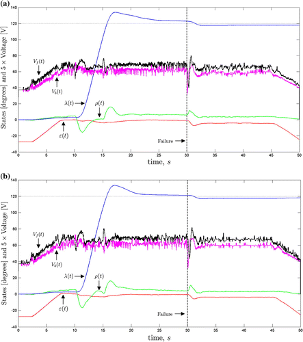
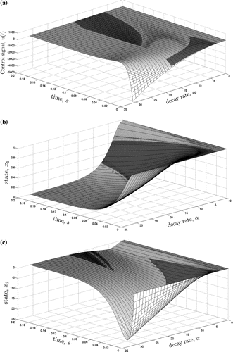
Finally, it was evaluated the behavior of the state variable (elevation $(\epsilon )$, pitch $(\rho )$, travel $(\lambda )$) and the voltages on the front and back motors, under a $50\%$ drop in power of the back motor (in the instant 30s) and attends the condition $||K||\approx 120$, as shown in Figure 5 (it is observed that application was limited to Theorems 3.1 and 4.1). Based on this figure, its notes a significant improvement in the state steady on the range of 0 to 30 seconds, due to the increase on the decay rate. There was also a little reduction in the altitude loss of the system after the failure application, without requiring high levels of electrical voltage in actuators, confirmed by signs $V_f(t)$ and $V_b(t)$.

Figure 5. Practical implementation of the designed K, (a) Theorem 3.1 and (b) Theorem 4.1.

Let us now to perform tests of impact on computational processing when an uncertainty (U) is added to the system. Thus, Table 2 illustrates the computational complexity required in terms of the number of scalar variables (V) and the number of LMIs lines (L). In this case, it’s evaluated the condition of $50\%$ drop in power of the back motor and $||K||\approx 250$. Later, it was added a new uncertainty to initial condition, i.e. the angle elevation belongs on the range of $\epsilon =-27.5^{\circ }(\approx -0.48rad)$ and $\epsilon =-1^{\circ }(\approx -0.0175rad)$.

Table 2. Numerical complexity to polytopic uncertains

Method	U	V	L
Theorem 3.1	1	53	53
	2	53	116
Theorem 4.1	1	153	86
	2	225	172
Theorem 5.1	1	153	102
	2	225	204

6.2. Mass-spring-damper

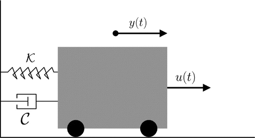
Consider a stabilizable system (Figure 6), described in (84).(84) $$\begin{array}{cc}\hfill \dot{x}(t)& =\left[\begin{array}{cc}0& 1\\ -\mathcal{K}& -\mathcal{C}\end{array}\right]x(t)+\left[\begin{array}{c}0\\ 1\end{array}\right]u(t)\hfill \\ \hfill y(t)& =[10]x(t)\hfill \end{array}$$(84)

where $-\mathcal{K}\in [-1.2,-0.8]$ and $-\mathcal{C}\in [-2.2,-1.8]$ are uncertain parameter, in appropriate units.

Figure 6. Mass-spring-damper system.

Let u(t) the action of the external force, $x_1(t)$ the position and $x_2(t)$ the speed of the mass. Therefore, the uncertain system based on norm-bound LDIs is described by,(85) $$\begin{array}{cc}\hfill \dot{x}(t)& =\left(\left[\begin{array}{cc}0& 1\\ -1& -2\end{array}\right]+\left[\begin{array}{cc}0& 0\\ 0.2& 0.2\end{array}\right]\left[\begin{array}{cc}{\lambda }_1& 0\\ 0& {\lambda }_2\end{array}\right]\left[\begin{array}{cc}1& 0\\ 0& 1\end{array}\right]\right)x(t)+Bu(t)\hfill \\ \hfill y(t)& =[10]x(t)\hfill \end{array}$$(85)

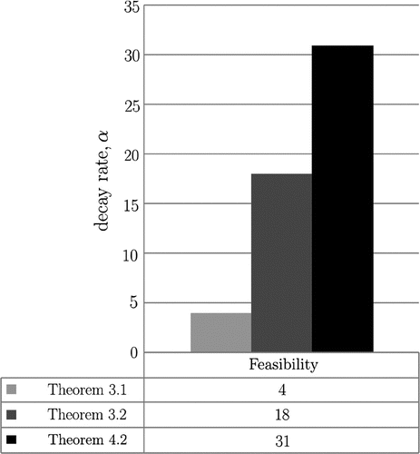
Weight matrices of the performance index are $\mathcal{R}=10$ and $\mathcal{Q}=\text{diag}(1,1)$, with the initial condition $x_0={[10]}^{\prime }$. It is observed that ${\lambda }_1={\lambda }_2=0$ implies in the nominal system. Moreover, in Figure 7, can be seen a performance analysis through feasibility regions, where it can be concluded that through the combination between Finsler Lemma and S-Procedure, applied to norm-bounded uncertain, it is ensures a largest bound on the decay rate. Furthermore, under the same conditions, the Theorem 3.2 ensured a greater feasibility region in controllers design than Theorem 3.1.

Figure 7. Number of feasibility regions for uncertainty models.

The computational complexity of the algorithm based on uncertain models is illustrated in Table 3. Thus, based on this table, it is noted that the L variable of Theorem 3.1 is equivalent to Theorem 4.2, however, the upper limit of the decay rate for norm-bounded uncertain is more advantageous than polytopic uncertain.

Table 3. Numerical complexity for uncertainty models

Method	U	V	L
Theorem 3.1	2	6	25
Theorem 3.2	2	8	14
Theorem 4.2	2	15	28

We, finally, consider the state and control signals applied to the nominal system in (84), as show in Figure 8. In this case, the Theorem 4.2 presented disadvantages as overshoot in control signals, i.e. a greater effort in the actuators; however, there was an improvement in the state steady with low decay rate.

Figure 8. Responses to control and states signals in function of the decay rate (dark gray surface: Theorem 3.2; white surface: Theorem 4.2).

7. Conclusions

In this study, less conservative LMIs formulations are proposed to synthesize linear robust quadratic regulators based on state feedback and applied to uncertain models most relevant in the literature. The proposals presented in this work allow us to set a bound of decay rate in the complex plane of $\lambda$-eigenvalues, from which the designers in control systems can perform a fine tune through the matrix $\mathcal{Q}$, and, consequently, to improve the temporal behavior of the interest signals. A numerical example illustrate the advantages of norm-bounded uncertainties in terms of implementation cost and of the limit variation in decay rate, and at the 3-DOF practical application, the controllers designed by Finsler and Reciprocal Projection lemmas increase the feasibility regions for systems subject to structural failure, guaranteeing robust stability and reduced controller’s norm when using parameter-dependent Lyapunov functions.

Cover image

Source: Quanser‘s 3-DOF helicopter of LPC - UNESP.

Additional information

Funding

The authors acknowledge the support of Fundação de Amparo à Pesquisa do Estado de São Paulo (FAPESP - Grant 2011/17610-0), Conselho Nacional de Desenvolvimento Científico e Tecnológico (CNPq - Research Fellowships 301227/2017-9 and 310798/2014-0), and Coordenação de Aperfeiçoamento de Pessoal de Nível Superior (CAPES).

Notes on contributors

Rodrigo da Ponte Caun

The research group has working in several areas of dynamical control systems. More specifically, it has addressed topics such as identification of dynamic systems, robust control, gain scheduling control, state derivative feedback control, switched systems, variable-structure control, control of nonlinear systems based on fuzzy models and design of control systems using Linear Matrix Inequalities (LMI). In this context, this paper has obtained original results for controllers design based on Linear Quadratic Regulators (LQR) using modern techniques of optimization and relaxation based on LMI. The main contribution involves the design of robust controllers applied to uncertain dynamic systems under a certain decay rate. Furthermore, the research group has working with several students at undergraduate, master’s and doctoral levels, as well as disseminating the results obtained in research in the form of scientific publications in periodicals or conferences.

References

- Apkarian, P. , Tuan, H. D. , & Bernussou, J. (2001). Continuous-time analysis, eigenstructure assignment, and H2 synthesis with enhanced linear matrix inequalities (LMI) characterizations. IEEE Transactions on Automatic Control , 46 , 1941–1946.
- Assunção, E. , Teixeira, M. C. M. , Faria, F. A. , Silva, N. A. P. D. , & Cardim, R. (2007). Robust state-derivative feedback LMI-based designs for multivariable linear systems. International Journal of Control , 80 , 1260–1270.
- Azizi, S. , Torres, L. A. B. , & Palhares, R. M. (2017). Regional robust stabilisation and domain-of-attraction estimation for MIMO uncertain nonlinear systems with input saturation. International Journal of Control , 91 (1), 1–14.
- Bombois, X. (2000). Connecting prediction error identification and robust control analysis: A new framework (Doctoral dissertation). Universite Catholique de Louvain.
- Boyd, S. , Ghaoui, L. , Feron, E. , & Balakrishnan, V. (1994). Linear matrix inequalities in system and control theory. In Studies in applied mathematics ( Vol. 15, 2nd ed.). Philadelphia, PA: SIAM.
- Buzachero, L. F. S. , Assunção, E. , Teixeira, M. C. M. , & da Silva, E. R. P. (2012). New techniques for optimizing the norm of robust controllers of polytopic uncertain linear systems. In G.L.O. Serra (Ed.), Frontiers in advanced control systems (pp. 75–100).
- Castelan, E. B. , Tarbouriech, S. , da Silva Jr., J. M. G. , & Queinnec, I. (2006). L2-Stabilization of continuous-time linear systems with saturating actuators. International Journal of Robust and Nonlinear Control , 16 , 935–944.
- Chancelier, J.-Ph. , Pakshin, P. V. , & Soloviev, S. G. (2011). LMI parser for NSP software package. IFAC Proceedings Volumes , 44 , 14253–14258.
- Chilali, M. , & Gahinet, P. (1996). H infty design with pole placement constraints: An LMI approach. Automatic Control: IEEE Transactions , 41 , 358–367.
- Corrêa, G. O. , & Freire, E. S. (2008). Robust H2 control based on dynamic multipliers. International Journal of Control , 81 , 1831–1848.
- Daafouz, J. , & Bernussou, J. (2001). Parameter dependent Lyapunov functions for discrete time systems with varying parametric uncertais. Systems & Control Letters: Elsevier Science , 43 , 355–359.
- Dallali, H. , Lee, J. , Tsagarakis, N. G. , & Caldwell, D. G. (2015). Experimental study on linear state feedback control of humanoid robots with flexible joints. IFAC-PapersOnLine , 48 , 130–135.
- da Silva, E. R. P. , Assunção, E. , Teixeira, M. C. M. , Faria, F. A. , & Buzachero, L. F. S. (2011). Parameter-dependent Lyapunov functions for statederivative feedback control in polytopic linear systems. International Journal of Control , 84 , 1377–1386.
- de Oliveira, M. C. , & Skelton, R. E. (2001). Stability tests for constrained linear systems. In S. O. Moheimani (Ed.), Perspectives in robust control. Lecture notes in control and information sciences (pp. 241–257). Berlin: Springer-Verlag.
- de Souza, C. E. , & Trofino, A. (2010). An LMI approach to stabilization of linear discrete-time periodic systems. International Journal of Control , 73 , 696–703.
- Faria, F. A. , Assunção, E. , Teixeira, M. C. M. , Cardim, R. , & da Silva, N. A. P. (2009). Robust state-derivative pole placement AaLMI-based designs for linear systems. International Journal of Control , 82 , 1–12.
- Fischer, J. , & Bhattacharya, R. (2009). Linear quadratic regulation of systems with stochastic parameter uncertainties. Automatical , 45 , 2831–2841.
- Ge, M. , Chiu, M. , & Wang, Q. (2002). Robust PID controller design via LMI approach. Journal of Process Control , 12 , 3–13.
- Geromel, J. C. , & Korogui, R. H. (2006). Analysis and synthesis of robust control systems using linear parameter dependent Lyapunov functions. IEEE Transactions on Automatic Control , 51 , 1984–1989.
- Gritli, H. , & Belghith, S. (2017). Robust feedback control of the underactuated Inertia Wheel Inverted Pendulum under parametric uncertainties and subject to external disturbances: LMI formulation. Journal of the Franklin Institute , 1–42.
- Hamada, Y. (2016). Preview feedforward compensation: LMI synthesis and flight simulation. IFAC-PapersOnLine , 49 , 397–402.
- Khairy, M. , Elshafei, A. L. , & Emara, H. M. (2010). LMI based design of constrained fuzzy predictive control. Fuzzy Sets and Systems , 161 , 893–918.
- Kothare, M. V. , Balakrishnan, V. , & Morari, M. (1996). Robust constrained model predictive control using linear matrix inequalities. Automatica , 32 , 1361–1379.
- Kumar, E. V. , Raaja, G. S. , & Jerome, J. (2016). Adaptive PSO for optimal LQR tracking control of 2 DoF laboratory helicopter. Journal Applied Soft Computing , 41 , 77–90.
- Kunee, V. , & Banjerdpongchai, D. (2008). Robust constrained model predictive control for linear time-varying systems with norm-bounded uncertainty. In Electrical engineering/electronics, computer, telecommunications and information technology: ECTI-CON 2008: 5th international conference (pp. 589–592).
- Lee, S. M. , Park, J. H. , Ji, D. H. , & Won, S. C. (2007). Robust model predictive control for LPV systems using relaxation matrices. IET on Control Theory Appl , 1 , 1567–1573.
- Löfberg, J. (2004). YALMIP: A toolbox for modeling and optimization in MATLAB. In Proceedings of the IEEE International Symposium on Computer Aided Control Systems Design (pp. 284–289). Retrieved from http://control.ee.ethz.ch/joloef/yalmip.php
- Ollala, C. , Levya, R. , Aroudi, A.E. & Queineec, I. (2008). LMI control applied to non-minimum phase switched power converters. In IEEE International Symposium on Industrial Eletronics (pp. 154–159).
- Ollala, C. , Levya, R. , Aroudi, A. E. , & Queineec, I. (2009). Robust LQR control for PWM converters: An LMI approach. IEEE Transactions on Industrial Electronic , 56 (7), 2548–2558.
- Pakshin, P. V. , Emelianova, J. P. , & Mazurov, A. Y. (2012). An experience of using LMI technique in student projects. IFAC Proceedings Volumes , 45 , 472–477.
- Pandey, S. K. , Mohanty, S. R. , Kishor, N. , & Catalão, J. P. S. (2013). An advanced LMI-based-LQR design for load frequency control of an autonomous hybrid generation system. In Doctoral conference on computing, electrical and industrial systems: Technological innovation for the internet of things (pp. 371–381).
- Peres, P. L. D. , Geromel, J. C. , & Bernussou, J. (1993). Quadratic stabilizabitily of linear uncertain systems in convex-bounded domains. Automatica , 29 , 491–493.
- Priess, M. C. , Conway, R. , Choi, J. , Popovich, J. M., Jr , & Radcliffe, C. (2015). Solutions to the inverse LQR problem with application to biological systems analysis. IEEE Transactions on Control Systems Technology , 23 , 770–777.
- Quanser . (2002). 3-DOF helicopter. Reference manual . Retrieved from http://www.quanser.com/english/html/products/fs_product_echallenge.asp?
- Scherer, C. , & Weiland, S. (2005). Linear matrix inequalities in control . Delft University of Technology and Eindhoven University of Technology.
- Xie, W. (2008). Multi-objective infty/alpha -stability controller synthesis of LTI systems. IET: Control Theory Applications , 2 , 51–55.
- Yang, Y. , Wu, M. & Chang, Y. (2010). Linear matrix inequalities based on linear quadratic regulator for the H2/Hinf control of the inverter split air conditioner temperature. In International refrigeration and air conditioning conference (Paper ID 1039) (pp. 1–8).
- Yue, M. , An, C. , & Sun, J. (2016). Zero dynamics stabilisation and adaptive trajectory tracking for WIP vehicles through feedback linearisation and LQR technique. International Journal of Control , 89 , 2533–2542.