Numerical simulation of improved RHS column-to-I beam flange-plate bolted connections for avoiding tensile fracture

Abstract

In an attempt to find possible solution for avoiding premature occurrences of brittle fracture in rectangular hollow section (RHS) column-to-I beam connections, an improved type of connection was tested by authors. Instead of welding, the beam was connected to the flange plates by bolts, some distance away from the column face. A series of test was conducted on this improved RHS column-to-I beam flange-plate bolted connection, the results show that the improved connection does not fail by fracture as observed in the conventional connections and has a larger energy dissipation capacity. This paper describes the finite element modeling method employed to analyses both conventional welded RHS column-to-I beam and improved bolted connections. Three highly complex 3D finite element models are created, accounting for material nonlinearity, large deformation and contact behavior involved in the models. The connection models have been analyzed under some loading conditions up to failure. The comparisons with experimental data show that the finite element models have high level of accuracy and can be employed to further optimize the connection design. In addition, the ultimate moment capacity of this improved connection is found to be predicted by simple formulas based on an elementary plastic analysis, and the connection has sufficient overstrength to allow formation of plastic hinges at the beam ends.

Keywords:

• through diaphragm
• wide flange beam
• RHS column
• bolted connections
• dissipated energy
• finite element simulation
• fracture
• validation

PUBLIC INTEREST STATEMENT

A series of tests is conducted on an improved rectangular hollow section (RHS) column-to-I beam bolted connection. The primary purpose of the tests is to find possible solutions for avoiding premature occurrence of brittle fracture. After the tests on both conventional and improved connections, it is found that fractures in connections do not occur in the improved connection and a larger energy dissipation capacity is achieved. However, because of the high costs of experiment, the number of tests is limited. Even if the cost is not a main concern, the experiments are generally limited the variation of a few parameter that have the most effect upon the connection behavior. A partial solution to this problem is to use finite element packages to model additional variations in parameters.The main aim of this paper is to validate the finite element method. Comparsions with experimental data show that the models have high levels of accuracy and can be employed in parametric study to develop more new connections avoiding premature occurrenc of brittle fracture.

1. Introduction

Although engineers believed that the joints between the beam flanges and columns using Complete Joint Penetration (CJP) groove welds satisfy adequate over-strength criteria to allow formation of plastic hinges in beam span and away from the face of column (CEN, 1994; ICBO, 1994), the 1995 Kobe earthquake in Japan revealed that the conventional types of rectangular hollow section (RHS) column-to-I beam connections in building frames were vulnerable to brittle fracture under the strong ground motion. After the earthquake, improvements of connection design were proposed. One way to achieve sufficient strength of connections is to reinforce the beam ends by adding additional members or plates (Chen, Lin, & Tsai, 2004). Another alternative approach is to reduce the cross section of the beam intentionally to produce an intended plastic hinge zone located away from the column face (Kurobane, 1998).

The above two strengthening approaches were developed by some researchers (Engelhardt, Winneberger, Zekany, & Potyraj, 1997), the laboratory tests showed excellent plastic deformation capacity. Inspired by these experiment results, authors conducted an improved RHS column-to-I beam bolted connection, the connection detail is to use bolted connections in place of welded connections in order that the critical section is move away from the column face, the brittle fracture may be avoided. After a series of tests on both conventional and improved connections, it was found that fractures in connections did not occur in the improved connection and also a larger energy dissipation capacity was achieved.

Experiment tests in general can provide reliable results that can describe the behavior of the beam-to-column connection. However, experimental work that involves high costs, and in some cases, is not feasible. Since numerical methods offer more flexibility and possibility to investigate a wider range of parameters than experiments can cover, the research on beam-to-column connections can be further extended using the finite element method (FEM).

The main objective of this work is to validate the FEM by comparing the simulated results with the experimental results. This paper first reviews the experimental procedure and failure modes of the connections, and then describes the finite element model that is used to analyze the connections. The ABAQUS finite element package is used to simulate the improved RHS column-to-I beam flange-plate bolted connection behavior observed in the tests performed at Kumamoto University in Japan. The results obtained from the finite element analyses are evaluated by comparing the moment-rotation responses with those of the corresponding tests.

2. Specimen and test program (Wu, 2000; Wu et al., 1999)

2.1. Specimen design

In order to compare different test results, specimens are made in two types: T-1, and T2 and T-3, as shown in Figure 1. T-1 is a conventional connection type (welded joints), with _ENDM_u ≥ 1.3M_p , where _END M_u is the ultimate flexural capacity of the specimen and M_p is the full plastic moment of the beam; T-2 and T-3 (welded and bolted joints in combination) are the improved types, with _ENDM_u  = α( _fM_u ,+  _wM_p ), where _fM_u is the ultimate moment of the beam flange, _wM_p is the plastic moment of the beam web, and

$\alpha =\frac{L{\hspace{0.17em}}_p^{\hspace{0.17em}}+L_h+L_t}{L_h+L_t}$

in which the lengths L_h, L_p and L_t are shown in Figure 1.

Figure 1. Specimen design.

2.2. Specimen details

Figure 2 illustrates the connection details for the bolted and welded connections of specimen. In each of these specimens, a wide flange beam with nominal dimensions of 500 mm × 200 mm (beam height × flange width) is welded to a cold-formed square hollow section column with nominal dimensions of 400 mm × 400 mm (column width × depth) to form a T-shaped subassembly. All the specimens have through and/or internal-diaphragms plates at the positions of the beam flanges to transmit axial forces in the flanges to the columns.

Figure 2. Connection details.

In specimen T-1, the beam web is welded to the column flange, and both beam flanges are welded to the through-diaphragm plates, and specimen T-2 and T-3 have through-diaphragm plate at the position of the beam top flange and internal-diaphragm plate at the position of the beam bottom flange. At the position of internal-diaphragm plate, a flange plate with bolt holes is butt-welded, which was connected to the beam bottom flange by the single-shear high-strength bolted joint. The flange-plate, which is used in specimen T-2, is a trapezoidal plate with dimensions of 230 mm× 200 mm× 445 mm (bottom width × top width× height), and the flange-plate, which is used in specimen T-3, is a rectangular plate with dimensions of 407 mm× 200 mm (length × width). The beam top flange is welded to the through-diaphragm plate while the beam web is bolted to the shear tab by a doubt row of eight bolts (T-2) or a single row of five bolts (T-3). The shear tab is welded to the column flange while it is also welded directly to the diaphragm plate and to the flange plate (T-2) in order to restrain rotation of the shear tab. The details see Figure 2.

2.3. Material properties

All the tensile uniaxial tests are done to the samples taken from one section of the beam and column. The mechanical properties of the materials are summarized in Table 1. All the materials are of weld-able low-carbon steel as specified by the Japanese Industrial Standards (JIS) SS400 and STKR400, roughly equivalent to the US ASTM A36 and A501 steels.

Table 1. Mechanical properties of materials

Location	σy (N/mm^2)	σu (N/mm^2)	E.L%	E (GPa)	Y.R	t (mm)	Specimen
Beam flange	306	448	23	212	0.68	15.45	T-1～T-3
Beam web	331	447	25	208	0.74	9.72	T-1～T-3
Column	338	439	22	202	0.77	11.48	T-1～T-3
Fin plate16mm	311	467	25	207	0.67	15.96	T-1～T-3
Diaphragm and flange plate19 mm	263	441	30.1	216	0.68	18.47	T-1～T-3

Note: σ_y  = yield stress; σ_u  = ultimate tensile strength stress; E.L. = elongation; E = elastic modulus; Y.R. = yield ratio(σ_y /σ_u ); t = thickness.

2.4. Test set-up

The loading arrangements are shown in Figure 3. Displacements taken from measurements are not only the horizontal displacement, u ₁, at the loading point but also the vertical displacement, v ₁ and v ₂, at the diaphragms and the horizontal displacement, u ₂, at the column end. The rotation of beam, θ_m , is calculated by the following equation:

${\theta }_{\mathrm{m}}=\frac{u_1-u_2}{L}-\frac{v_2-v_1}{J_d}$

where L and J_d denote the distance from the loading point to the column face and the distance between the centroids of the top and bottom diaphragms, respectively.

Figure 3. Test set-up.

All the specimens are subjected to a displacement controlled loading history based on the protocol recommended by SAC (SAC Steel Project, 1997) at rate of 2 in. per minute and are tested as follows: at least two cycles of reversed loading in an elastic region and, subsequently, a displacement controlled cyclic loading with the amplitude increased as ± 2θ_p , ± 4θ_p , ± 6θ_p ,…, until a failure occurs, where θ_p represents the elastic beam rotation at the full plastic moment M_p (see Appendix B) (Wu, 2000; Wu et al., 1999; Kurobane., 1998), and can be calculated by the following equation:

${\theta }_{\mathrm{p}}=\frac{L}{3EI}{M}_p+\frac{1}{G{A}_w}\frac{M_p}{L}$

Two cycles of the loading are applied at each displacement increment.

2.5. Test results

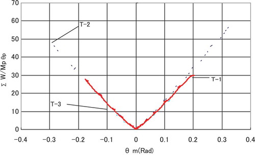
Figure 4 shows the bending moment vs. beam rotation hysteric curve at the column face. The moment is the maximum moment at the column face, M_m , and is non-dimensionalized by the full-plastic moment, M_p , of the beam. The moment takes positive value when the bottom flange is in tension. The rotation, θ_m , denotes the rotation of the beam segment between the loading point and the column face (see Appendix B). Tables 2–4 show the failure sequences of specimens.

Table 2. Failure sequences of specimen T-1

Sequence no.	Mm /Mp	Mm	θm	Detail
1	1.13	730	2.1 × 10^−2	Hair crack (bottom flange)
2	−1.15	740	2.1 × 10^−2	Crack (top flange) = 1mm
3	1.26	810	3.1 × 10^−2	Crack (bottom cope), crack (web), buckle (top flange)
4	−1.24	799	3.1 × 10^−2	Crack (top cope), buckle (bottom flange)
5	1.29	830	3.1 × 10^−2	Crack (bottom flange) = 4mm, crack (bottom cope) = 1mm
6	−1.10	712	3.8 × 10^−2	Crack (top flange) = 40mm
7	0.51	328	2.7 × 10^−2	Crack (bottom flange) = 30mm, through crack (bottom cope)

Figure 4. Moment vs. beam rotation hysteric curves.

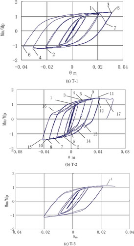
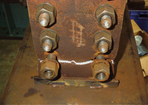
Three failure modes are identified in this test: (1) the tensile failure of the beam flange at the beam end (T-1, see Figure 5); (2) the local buckling of the plate element at the beam end (T-2, see Figure 6); and (3) the tensile failure of the flange plate at the position of the first bolts nearest to the column (T-3, see Figure 7). For specimen T-1, first, cracks are found either at the tip of the weld toes or at the toe of the beam cope. Then, these cracks grow gradually with load cycling and finally lead to tensile failure of the beam flange. For specimen T-3, the size of the flange plate is insufficient (Figure 2), which lead to the flange plate rupture at the first bolt hole. However, T-2, which is designed to have sufficient tensile capacity at the flange ends, reaches the maximum loads, but only leading to local buckling of the top flanges and the web of the beams.

Figure 5. Tensile failure T-1.

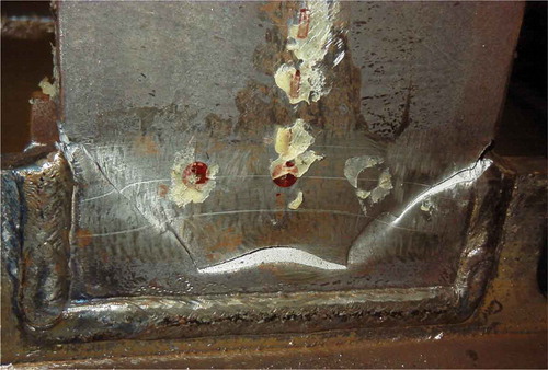
Figure 6. Local buckling observed in T-2.

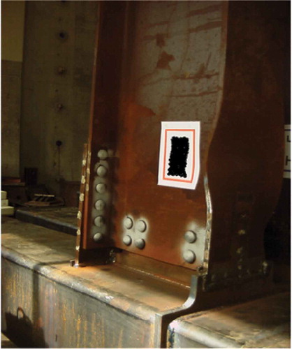
Figure 7. the flange plate rupture (T-3).

2.6. Discussion of test result

Specimen T-1 has welded joints at both the top and bottom flanges, while specimens T-2 and T-3 have welded joint at top flange and bolted joint at the bottom flange. Comparison is made of the deformation capacities between the two types in term of dissipated energy. The definition of dissipated energy is shown in Appendix B. The area below the hysteresis curve represents the dissipated energy. However, since the area below an elastic unloading envelope represents the energy stored in the structure, this area is regarded as the negative dissipated energy. The dissipated energies, non-dimensionalized by M_pθ_p , are plotted against the accumulated beam rotation Σθ_m for these two types of specimens in Figure 8, where Σθ_m is the sum of rotations caused by either the positive or negative moment. Comparison the capacity of dissipated energies that are shown in Figure 8, it can be seen that dissipated energies at the same Σθ_m are almost identical for the conventional type and improved type. However, the final dissipated energy is much greater for the improved type (T-2) than for the conventional type (T-1). Additionally, conventional connections usually sustained brittle fracture by fast cracks beginning from the tips of ductile cracks. Representative locations where ductile cracks initiates are firstly at the toes of beam cope, secondly, at the weld tab regions. The cumulative plastic deformation factor, ηthat can be expected to be achieved when the failure occurs is 50. However, for the improved specimen T-2, although the cracks described above are found, the crack growth is stable, finally, these cracks extended only 2 mm. The cumulative plastic deformation factors (η) is 119, much greater than that of the conventional connection.

Figure 8. Dissipated energy during load cycling.

3. Finite element analyses (FEA) (Wu & Feng, 2013)

3.1. Finite element model

A three-dimensional finite element model of the RHS column-to I beam connection is created using the HYPERMESH (Altair) pre-processor. The connections are analyzed using the ABAQUS finite element software package.

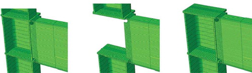
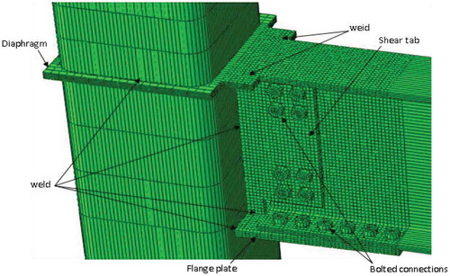
The finite element mesh used in the analyses is shown in Figure 9. The detail mesh of bolted connection sees Figure 10. The mesh contains approximately 34,318 nodes and 28,092 elements. In the mesh generation, the connection is divided into seven individual components, which are shown in Figures 11 and 12, and are referred to as the column, beam, flange plate, diaphragm, bolt, share tab and weld.

1. Column, beam, diaphragm, shear tab and flange plate

Figure 9. Finite element mesh.

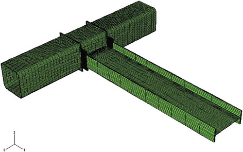
Figure 10. Detail mesh of bolted connection.

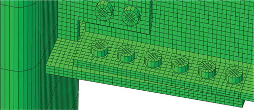
Figure 11. Mode components (T-1).

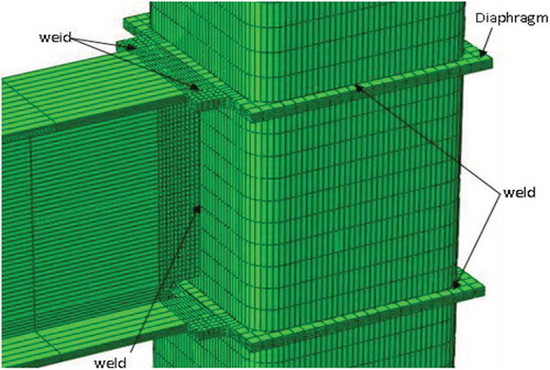
Figure 12. Mode components (T-2).

The column, beam, diaphragm, shear tab and flange plate are modeled using 3-D 8-node brick elements. Linear hybrid elements are selected to prevent the possible problem of volumestrain locking. Following a convergence study, three elements through the thickness of the diaphragm, flange plate and beam flange are used. Furthermore, to reduce the number of elements and nodes in the FE model, only one element is used for the column, beam web and shear tab through their thickness.

• (2) Weld

There are two types of welding. One type is the filled weld, applied to the shear tab-to-column, shear tab-to-flange plate and shear tab-to-diaphragm plate. The other is groove weld, applied to the diaphragm-to-column, beam-to-diaphragm and flange plate-to-column. In the finite element model, the weld is assumed to be an extension of the diaphragm sections, the column sections, flange plate and the shear tab section, therefore has the same material properties as the connection. Consequently, the weld is modeled as an individual component in the connection model using 8-node brick elements.

• (3) Bolt

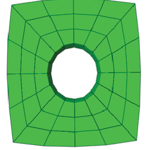
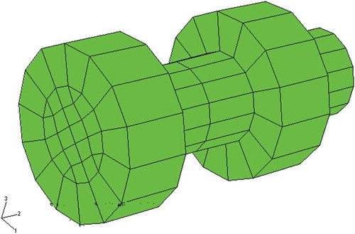
The bolt model is constructed using 8-node brick elements and 6-node triangular prism elements, as shown in Figure 13. The bolt connections include three main parts: beam, flange plate or shear tab and bolts. To capture the accurate stress behavior, an intensive mapped mesh is made around the boltholes (detail sees Appendix F). The hexagon bolt heads are modeled as cylinders.

Figure 13. Finite element model of bolt.

The small sliding interaction behavior between the contacting surfaces is considered for all the contact surfaces in order to fully transfer the loading from the beam web to the shear tab, and the beam flange to the flange plate, and then finally, to the column. The following contact interactions for the bolt connection are considered: (1) Contact between the bolt shank and the bolt hole; (2) Contact between the bolt head and the beam web or beam flange; (3) Contact between the nut and the shear tab or flange plate; and (4) Contact between the shear tab and the beam web, and the flange plate and beam flange. In the modeling, using “pretension section”adds to the bolt shank and the bolts are pre-loaded by a tensile force of 120 kN during the analysis and a friction coefficient $\mu$ = 0.45 is used for all the contact surfaces.

FEA involve two steps. Firstly, the pretension loads are applied to the bolts; secondly, a cycle of reversed load in an elastic region is applied at the loading point and, subsequently, a displacement controlled cyclic load is exerted as conducting in the experiment test. Although two cycles of loading are applied at each displacement increment in the experiments, in the numerical analyses, only one cycle for each displacement increment is exerted to the beam to save computational time.

3.2. Classical metal plasticity model

In this work, the classical metal plasticity constitutive model implemented in ABAQUS is adopted for its simplicity. The total strain rate is decomposed into the elastic and plastic components:

(1) $\dot{\epsilon }={\dot{\epsilon }}^{el}+{\dot{\epsilon }}^{pl}$(1)

where ${\epsilon }^{el}$ and ${\epsilon }^{pl}$ are elastic and plastic strain, respectively. Eq. (1) can be written in integrated form as

(2) $\epsilon ={\epsilon }^{el}+{\epsilon }^{pl}$(2)

The elasticity is linear and isotropic, and is written in terms of the bulk modulus, $K$, and the shear modulus, $G$, as follows

(3) $p=-K{\epsilon }_v,\mathbf{S}=2G{\mathbf{e}}^{el}$(3)

with

(4) $K=\frac{E}{3\left(1-2\nu \right)},G=\frac{E}{2\left(1+\nu \right)}$(4)

where $p=-1/3\mathrm{t}\mathrm{r}\mathrm{a}\mathrm{c}\mathrm{e}(\sigma )$ is the equivalent pressure stress; ${\epsilon }_v=\mathrm{t}\mathrm{r}\mathrm{a}\mathrm{c}\mathrm{e}(\epsilon )$ is the volumestrain; $\mathbf{S}=\sigma +p\mathbf{I}$ is the deviatoric stress; and ${\mathbf{e}}^{el}={\epsilon }^{el}-1/3{\epsilon }_v\mathbf{I}$ is the elastic deviatoric strain.

The von Mises yield criterion with isotropic hardening behavior is assumed:

(5) $f\left(\sigma \right)=\sqrt{\frac{3}{2}\mathbf{S}:\mathbf{S}}={\sigma }^0({\bar{\epsilon }}^{pl})$(5)

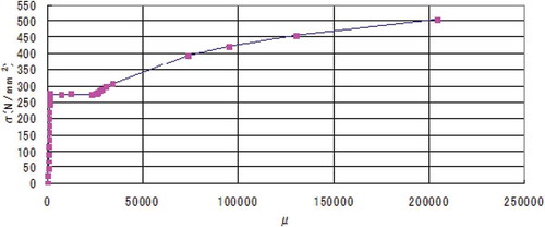
where ${\sigma }^0$ is the yield stress and is defined as a function of equivalent plastic strain $\bar{\epsilon }{}^{pl}$. It can be determined according to the stress–strain relation measured from uniaxial tensile experiments, as shown in Figure 14.

Figure 14. Steel stress–strain curve.

The associated flow rule is used in the model and has the following form

(6) $d{\epsilon }^{pl}=d{\bar{\epsilon }}^{pl}\mathbf{n}$(6)

with

(7) $\mathbf{n}=\frac{3}{2}\frac{\mathbf{S}}{f\left(\sigma \right)}$(7)

Eqs. (2)–(7) define the metal material behavior. These equations are required to be integrated and solved when plastic flow occurs. The integration is done by applying the backward Euler method to the flow rule, and then a nonlinear equation is established by combining the equations with the integrated flow rule. The nonlinear equation is solved by Newton’s method and the metal plasticity behavior is determined.

For the ABAQUS simulation, the nominal engineering stress-strain relation obtained from steel tensile coupon test (see Table 1) is converted to the true stress-strain relationship, according to: ${\sigma }_{\mathrm{t}\mathrm{r}\mathrm{u}}={\sigma }_{\mathrm{n}\mathrm{o}\mathrm{m}}(1+{\epsilon }_{nom})$ and ${\epsilon }_{\mathrm{t}\mathrm{r}\mathrm{u}}=ln(1+{\epsilon }_{\mathrm{n}\mathrm{o}\mathrm{m}})$, in which ${\sigma }_{\mathrm{t}\mathrm{r}\mathrm{u}}$ and ${\epsilon }_{\mathrm{t}\mathrm{r}\mathrm{u}}$ represent the true stress and strain; and ${\sigma }_{\mathrm{n}\mathrm{o}\mathrm{m}}$ and ${\epsilon }_{\mathrm{n}\mathrm{o}\mathrm{m}}$ are the nominal stress and strain respectively. The true stress–strain relationship sees Appendix D.

3.3. Analysis results

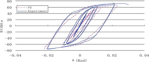
The numerical analyses of specimens are terminated when the connections fail with the maximal rotation 6θ_p (except for T-3, roughly 5θ_p ). Figures 15–17 show both the simulated and experimental results, and reveal that when the beam tip rotation is between 4θ_p and −4θ_p , the experimental and numerical loops match well. However, when the rotation is over 4θ_p and −4θ_p , the numerical loops overestimate the stiffness of the specimens. The difference between the experimental and numerical loops is likely caused by the difference between the nominal and measured material properties and inaccurate measurement of the specimen dimensions. In addition, during the tests, it is very difficult to induce a predetermined bolt force by pretension techniques because the bolt forces are very high (Shi, Shi, Wang, & Bradford, 2008), this may be also a reason for the difference between the experimental and numerical results.

Figure 15. Hysteresis curves (T-1).

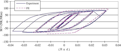
Figure 16. Hysteresis curves (T-2).

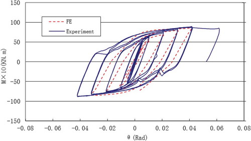
Figure 17. Hysteresis curves (T-3).

The moment–rotation relationships for specimens T-1, T-2 and T-3 analyzed by FEM are shown in Figure 18, in which the curves, test1-1(FE), test2-1(FE) and test3-1(FE) are obtained from the FE analyses, and test1, test2 and test3 are obtained from the so-called skeleton curves. The skeleton curve is constructed from a hysteretic curve by linking a portion of the curve that exceeds the maximum load in the preceding loading cycle sequentially (see Appendix C). Comparison of the FE results with the experimental moment–rotation curve (see Figures 19–21) shows good agreement in terms of general behavior and the maximum values with a difference around 10%. An observation of FE failure mode shows a similarity to the test results (see Figures 5–7 and 22–24).

Figure 18. Moment–rotation relationships.

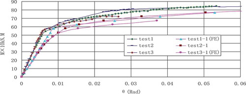
Figure 19. T-1 Moment–rotation relationships.

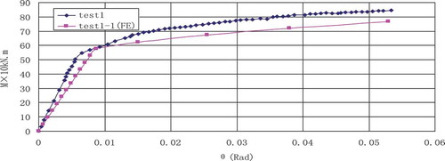
Figure 20. T-2 Moment–rotation relationships.

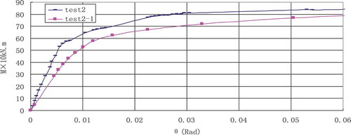
Figure 21. T-3 Moment–rotation relationships.

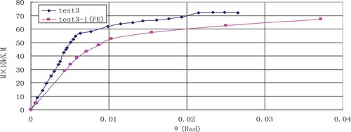
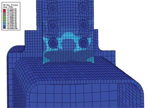
Figure 22. T-1 Plastic strain distribution.

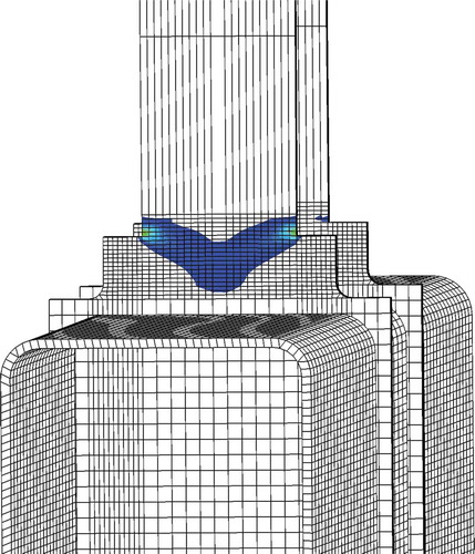
Figure 23. FE analyses result of the beam top flange buckling (T-2).

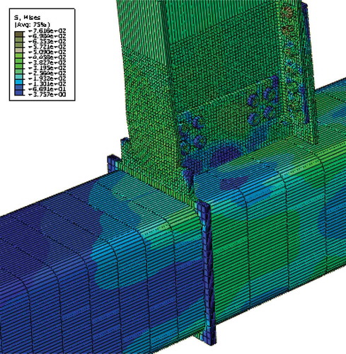
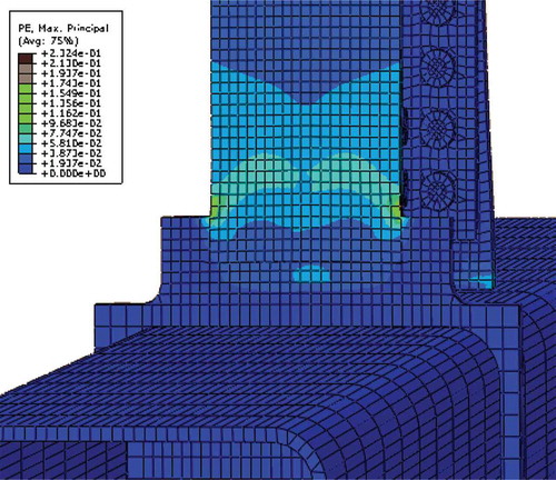
Figure 24. T-3 Plastic strain distribution under the cyclic load.

3.4. Comparison of results

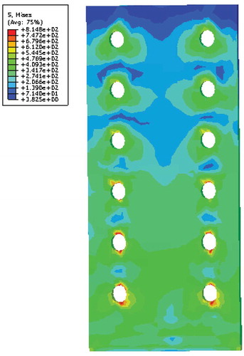
Figure 25 illustrates the plastic strain distribution under cyclic load in T-2. Comparison FEA results of the specimens T-1, T-2 and T-3 that are shown in Figures 22, 24 and 25, it can be seen that the plastic hinge occurs within the beam span and away from the column face in specimen T-2. This may be the reason why the tensile fracture is prevented. However, for specimen T-3, as the flange plate size is smaller than specimen T-2, which leads to the fracture in the first bolt, and for specimen T-1, it is the tensile failure at the beam flange.

Figure 25. T-2 Plastic strain distribution under the cyclic load.

3.5. Additional results in the bolt pre-tensioned flange-plate joints

The FEA study can obtain numerously valuable results for bolt pre-tensioned flange-plate joints, which are difficult to measure in experimental tests.

Figure 26 shows the distribution of pressure between the flange plate and the beam bottom flange before loading.

Figure 26. Distribution of pressure between the flange-plate and beam bottom flange caused by bolt pretension force.

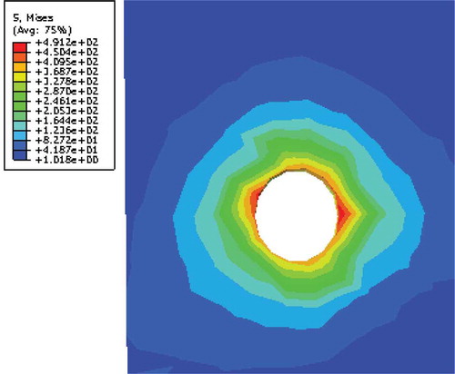
Figures 27 and 28 illustrate the distribution of the force between the flange-plate and beam bottom flange at the ultimate load for joints in specimens T-2 and T-3, respectively.

Figure 27. Distribution of force between the flange-plate and beam bottom flange at the ultimate load (T-2).

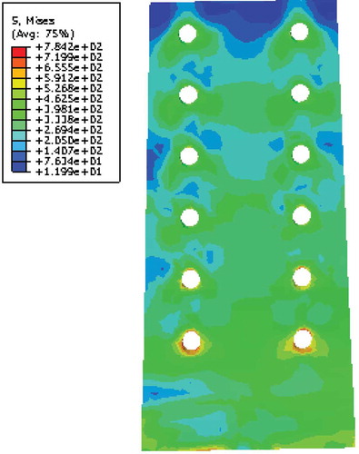
Figure 28. Distribution of force between the flange-plate and beam bottom flange at the ultimate load (T-3).

These results provide important information in theoretical analysis of the overall behavior of bolted connections of this type. About more details, please see Ref. Shi, Shi, and Wang (2007), although it is for analysing end-plate connection, in some extent, there are very similar. A more detailed explanation is omitted here.

4. Evaluation of ultimate strength of connections

The ultimate strength of these connections can be predicated by simple formulas based on some elementary plastic analyses.

4.1. Failure modes

Three failure modes are identified in the connection test: (1) the tensile failure of the beam flange at the beam end (T-1); (2) the local buckling of the plate element at the beam end (T-2); and (3) the tensile failure of the flange plate at the position of the first bolts nearest to the column (T-3).

4.2. Tensile strength of the welded joints

The fracture paths, which occur in specimen T-1, are shown in Figure 29. To predict the ultimate tensile strength of these joints, two fracture paths are proposed as follows (see Figure 30). L_p signifies the length of the welded joint, L_d signifies the space between the toe of beam cope and the beam end, L_s signifies the space between the beam end and column face, b denotes the width of the beam flange and b_e denotes the width of the welded joint.

Figure 29. Fracture paths at the beam end in tests.

Figure 30. Proposed fracture paths at the beam end.

Tanaka (1999) recommended the following formula for calculation the tensile strength of each fracture path when failure occurs by ductile tear along the fracture path (Fracture path 1),

(8) $P_u=L{\hspace{0.17em}}_f^{\hspace{0.17em}}\times t_f\times (sin\theta +\frac{cos\theta }{\sqrt{3}})\times {\sigma }_{f,u}$(8)

where L_f signifies the length of fracture path, σ_f,u is the ultimate tensile strength of the beam flange and t_f is the thickness of the beam flange.

Therefore, the ultimate moment carried by the flange M_f,u is evaluated as the axial capacity of one of the beam flange-to-column flange joints multiplied by the distance between the centroids of the top and bottom flange to column joints. Therefore, the flexural capacity of the beam at the column face M_f,u is given as

(9) $M_{f,u}=[b\times t_f\times {\sigma }_{f,u}+\frac{2}{\sqrt{3}}(L_p-L_d)\times t_f\times {\sigma }_{f,u}]\times \frac{J_b\times L}{L-L_p-L_s}$(9)

In general, the fracture path 2 is much stronger than the fracture path 1 and thus such a fracture is not necessary to be considered. However, to ensure a sufficient over-strength to prevent tensile failure, the optimum length of such welded joint can be calculated as

(10) $L_p=L{\hspace{0.17em}}_d^{\hspace{0.17em}}+\frac{\sqrt{3}}{2}(b_e-b)$(10)

Since specimen T-1 has a welded web joint, the bending moment carried by this joint should be added to the moment given by Eq. (9) to evaluate the ultimate flexural capacity of connection. AIJ (1996) proposed the following formula for the flexural capacity,

(11) $M_{w,u}=(x-S_v)(H_b-t_f-x-S_v)f_w$(11)

where x is obtained by a yield line analysis and is given by

(12) $x={\left(\frac{t_c^2(H_b-t_f){\sigma }_{w,y}}{f_w}+S_v^2\right)}^{1/2}$(12)

in which H_b denotes the height of the beam, t_c is the thickness of the beam flange, S_v is the vertical space of the beam cope (see Figure 31) and f_w signifies the stress and is given as the smaller of the following two values,

(13) $f_w=t_w{\sigma }_{w,y}{f}_w=\frac{2}{\sqrt{3}}{t}_c{\sigma }_{c,y},$(13)

where t_w denotes the thickness of the beam web, σ_w,y is the yield strength of the beam web and σ_c,y is the yield strength of the column.

Figure 31. Moment carried by welded web joint.

So, the ultimate flexural capacities _EndM_u is given as the following:

(14) ${\hspace{0.17em}}_{End}^{\hspace{0.17em}}{M}_u=M_{f.u}+M_{w.u}$(14)

4.3. Ultimate strength of the bolted joints

For specimens T-2 and T-3, the top flanges use the welded joints which are same as specimen T-1. Figure 32 shows the details. Unlike specimen T-1 which needs to consider the flexural capacity of the welded web joint, the flexural capacity of bolted web connection in specimens T-2 and T-3 can be neglected because of the large flexibility of the connection due to the bolt slip and local yielding of the column flange, so, the ultimate flexural capacity is given by,

(15) ${\hspace{0.17em}}_{End}^{\hspace{0.17em}}{M}_u=[b\times t_f\times {\sigma }_{f,u}+\frac{2}{\sqrt{3}}(L_p-L_d)\times t_f\times {\sigma }_{f,u}]\times (H_b-\frac{t_f}{2}+\frac{t_p}{2})\times \frac{L}{L-L_p-L_s}$(15)

In which t_p is the thickness of the flange plate.

Figure 32. Details of the flange–plate connection.

And, the width of the flange plate in the first bolt (b_p ) is governed by the follows:

(16) $b_p=\frac{{\hspace{0.17em}}_{End}^{\hspace{0.17em}}{M}_u\times (L-L_1)}{{\sigma }_{p,u}\times t_p\times L\times (H_b-\frac{t_f}{2}+\frac{t_p}{2})}+2d_0$(16)

Where L ₁ is the distance between the first bolts and column face, σ_p,u is the ultimate tensile strength of the flange plate and d ₀ signifies the diameter of bolt hole.

The ultimate flexural capacities _EndM_u  = M_f.u or _EndM_u = M_f.u + M_w,u of beam-to-column connections, determined by the tensile capacities of the welded joints at the beam ends, are summarized in Table 5 and compared with the test results. The table shows that the predictions agree well with the test results except for specimens T-3.

Table 3. Failure sequences of specimen T-2

Sequence no.	Mm /Mp	Mm	θm	Detail
1	1.05	634	1.1 × 10^−2	Flange plate slip = 2mm
2	−1.08	654	1.0 × 10^−2	Bolt slip
3	1.18	713	2.1 × 10^−2	Flange plate slip = 5mm
4	1.23	741	2.1 × 10^−2	Bolt slip (web)
5	1.32	797	3.1 × 10^−2	Flange plate slip = 8mm
6	−0.74	450	2.6 × 10^−2	Bolt slip (web)
7	−1.28	777	2.3 × 10^−2	Crack (top flange)
8	−1.33	806	3.2 × 10^−2	Crack (top flange) = 1.5mm
9	1.36	827	3.1 × 10^−2	Flange plate slip = 9mm
10	−1.34	811	3.1 × 10^−2	Buckle (bottom flange)
11	1.42	857	4.2 × 10^−2	Buckle (top flange)
12	1.44	870	4.2 × 10^−2	Flange plate slip = 10mm
13	−0.46	278	2.1 × 10^−2	Bolt slip
14	−0.78	471	9.9 × 10^−3	Bolt slip
15	−1.43	864	4.2 × 10^−2	Crack (top flange)
16	0.31	189	2.0 × 10^−2	Bolt slip
17	1.36	821	5.3 × 10^−2	Buckle (web)

Table 4. Failure sequences of specimen T-3

Sequence no.	Mm /Mp	Mm	θm	Detail
1	1.05	676	3.0 × 10^−2	rupture(flange plate in the first row of bolt hole)

Table 5. The tensile capacity comparison between the test and prediction results

Specimen	Test	Prediction			Mm / EndM u
	Mm (KN-m)	Mf,u (KN-m)	Mw,u (KN-m)	EndMu (KN-m)
T-1	830	781	55	836	0.99
T-2	864	848		848	1.02
T-3	676	904		904	0.75

For specimen T-3, as the width of the flange plate in the first bolt (b_p ) can not achieve the requirement, the specimen fails prematurely by tensile failure of the flange plate at the position of the first bolts. However, for specimen T-2, the size of the flange plate is sufficient and the fracture does not occur.

5. Conclusion

A FE analysis of the behavior of the RHS column-to-I beam flange-plate bolted connections is described in this paper. Three test specimens are simulated. The model includes the individual beams, columns, diaphragms, bolts, shear plate and the complex contact surfaces. Material nonlinearity is considered for all components. Contacts are critical to model the bolted connection behavior of the joint. Contact elements have been used at the bolt-hole and also at the surface between the web of the beam and shear plate, flange plate and beam flange; taking into consideration the pre-tension in the bolted connections and friction between the surfaces. Three-dimensional brick elements are employed as this type of element is easily adapted to model interfaces between the connecting surfaces. The comparison shows a good correlation between the FE and experimental results of the connection behavior. This proves that the FEM is capable of accurately predicting RHS column-to-I beam connection behavior. An improved type of RHS column-to-I beam connection model has successfully been created and validated against a series of test data. The methodology can be further parametric study of bolted connections, which can obtain comprehensive results in order to develop more new connections. In addition, for the improved flange plate connection which have welded joint at top flange and bolted joint at the bottom flange, it is recommended that the flange plate connection has the ultimate strength equal to or slightly greater than that of the welded joint. Futher, it is desirable that the flange plate is designed to be wider and thicker than the beam flange at the welded joint to the column. The cross sectional areas of the flange plate in specimen T-2 is greater than this of the beam flange by about 36%.

Acknowledgements

The experimental investigation was conducted in the former Makino lab, Kumamoto University, Japan. The authors wish to thank professor Makino who has retired from Kumamoto University for his help.

Additional information

Funding

The authors received no direct funding for this research.

Notes on contributors

J. Wu

Jian Wu is an associate professor at the College of Engineering Management, Guangxi University of Finance and Economics, China. He is a register Engineer. His research interests are structures and materials.

WG. Tong

Weiguang Tong is an associate professor at the College of Architecture and Civil Engineering, Guangxi University, China. His research interests are sustainable materials and structures.

Appendix A.

Symbols

A =	=	cross-sectional area (mm2)
E =	=	elastic modulus (Gpa)
σ =	=	strength (N/mm2)
G =	=	shear modulus of elasticity (Gpa)
H =	=	height (mm)
I =	=	moment of inertia (mm4)
J =	=	distance between centroids (mm)
L =	=	length (mm)
M =	=	bending moment (N·mm or KN·mm)
P =	=	force (N or KN)
t =	=	thickness (mm)
u =	=	horizontal displacement (mm)
v =	=	vertical displacement (mm)
θm =	=	rotation (radian)

Appendix B.

Definition of cumulative plastic deformation factor

The bending moment M_m represents the maximum beam moment at the column face. The rotation θ_m is the rotation of the beam segment between the loading point and the column face (see Fig. A1). The full plastic moment M_p is calculated by using the measured yield stresses of materials and measured dimensions of beam sections. The elastic beam rotation θ_p at the full plastic moment is defined as the elastic component of beam rotation at M_m  = M_p (see Fig. A2). The cumulative plastic deformation factor is defined as the sum of η_i ⁺ and η_i ⁻ by the specimen until failure occurs and written as:

$\eta =\sum _t({\eta }_i^{+}+\left|{\eta }_i^{-}\right|)$

The alternative definition of the cumulative plastic deformation factor is the sum of plastic energies dissipated during all the cycles, non-dimensionalized by dividing the energy by M_pθ_p . According to the latter definition η_i ⁺ and η_i ⁻ are written as:

${\eta }_i^{+}=\frac{\sum _i{W}_i^{+}}{M_p{\theta }_p}\mathrm{a}\mathrm{n}\mathrm{d}{\eta }_i^{+}=\frac{\sum _i{W}_i^{-}}{M_p{\theta }_p}$

Where w_i denotes the energy absorbed at the I-th cycle (see Fig. A2)

Appendix C.

Definition of skeleton curve

The skeleton curve is constructed from a hysteretic curve by linking a portion of the curve that exceeds the maximum load in the preceding loading cycle sequentially (see Fig. A3)

Appendix D.

The true stree–strain relationship

Appendix E:

Details of welded connection (T-1)

Appendix F:

The element used in critcial areas (Boltholes)

In this paper, the critical area is the bolt hole, and the area is defined 50 × 50 mm². The mesh of bolthole is shown in Fig. A6, it is divided into four equal trapezoidal areas by four lines extending from the center of bolt hole to the four corners of the square. Mesh 4 × 3 is used, because 4 × 3 will give a satisfactory solution if the requirement for accuracy is not very high (Yu, Burgesss, Davison, & Plank, 2008). The length of side of element size is around 4–12.5 mm.

References

- AIJ . (1996). The state of art report on the structure behavior of steel connection . (pp. 29–31). Tokyo, Japan: Architectural Institute of Japan. in Japanese.
- CEN . (1994). Eurocode 8-Design provisions for earthquake resistance of structure, part 1-1, 1-2,1-3. ENV 1998-1-1 , European committee for Standardization, 1–2, 1–3.
- Chen, C.-C. , Lin, C.-C. , & Tsai, C.-L. (2004). Evaluation of reinforced connections between steel beams and box columns. Engineering Structures , 26, 1889–1904. doi:10.1016/j.engstruct.2004.06.017
- Engelhardt, M. D. , Winneberger, T. , Zekany, A. J. , & Potyraj, T. J. (1997). The dogbone connection: Part II. Modern Steel Construction , 36(8), 46–55.
- Yu, H. X. , Burgesss, I. W. , Davison, J. B. , & Plank, R. J. (2008). Numerical simulation of bolted steel connections in fire using explicit dynamic analysis. Journal of Constructional Steel Research , 64, 515–525. doi:10.1016/j.jcsr.2007.10.009
- ICBO . (1994). Uniform building code . Whittier, CA: International Conference of Building Officials.
- Wu, J. (2000). Study of new RHS column-to-I beam connections for avoiding tensile fracture ( M.S thesis), Kumamoto University, Japan. (in Japanese).
- Wu, J. , Ikebata, K. , Kurobane, Y. , Makino, Y. , Ochi, K. , & Tanaka, M. (1999). Experimental study on RHS column to wide flange I-beam connections with external diaphragms (pp. 517–520). Hiroshima: AIJ. (in Japanese)
- Kurobane, Y. (1998). Improvement of I beam-to-RHS column moment connections for avoidance of brittle fracture, tubular structures VIII (pp. 3–17). ( Y. S. Choo & G. J. Van Der Vegte , Eds.). Rotterdam: Balkema.
- SAC Steel Project . (1997, October). Protocal for fabrication, inspection, testing, and dcumentation of beam-column connection tests and other experimential specimens. Report No. SAC/BD-97/02 . SAC Joint Venture.
- Shi, G. , Shi, Y. , Wang, Y. , & Bradford, M. A. (2008). Numerical simulation of steel pretensioned bolted end-plate connections of different types and details. Engineering Structures , 30, 2677–2686. doi:10.1016/j.engstruct.2008.02.013
- Shi, Y. , Shi, G. , & Wang, Y. (2007). Experimental and theoretical anaylsis of the moment-rotation behaviour of stiffened extended end-plate connections. Journal of Constructional Steel Research , 63, 1279–1293. doi:10.1016/j.jcsr.2006.11.008
- Tanaka, N. (1999). Study on structural behavior of square steel column to H-shaped steel beam connections ( Doctoral dissertation), Kumamoto University. (in Japanese).
- Wu, J. , & Feng, Y. T. (2013). Finite element simulation of new RHS column-to-I beam connection for avoiding tensile fracture. Journal of Constructional Steel Research , 86, 42–53. doi:10.1016/j.jcsr.2013.03.012
- HKS. (2001), ABAQUS Users1490147 Manuals v 6.2 . Hibbitt. Karisson and Sorenson Inc.