A review of multi-objective optimization: Methods and its applications

Abstract

Several reviews have been made regarding the methods and application of multi-objective optimization (MOO). There are two methods of MOO that do not require complicated mathematical equations, so the problem becomes simple. These two methods are the Pareto and scalarization. In the Pareto method, there is a dominated solution and a non-dominated solution obtained by a continuously updated algorithm. Meanwhile, the scalarization method creates multi-objective functions made into a single solution using weights. There are three types of weights in scalarization which are equal weights, rank order centroid weights, and rank-sum weights. Next, the solution using the Pareto method is a performance indicators component that forms MOO a separate and produces a compromise solution and can be displayed in the form of Pareto optimal front, while the solution using the scalarization method is a performance indicators component that forms a scalar function which is incorporated in the fitness function.

Keywords:

• multi-objective optimization
• Pareto
• scalarization
• dominated solution
• non-dominated solution

PUBLIC INTEREST STATEMENT

Multi-objective optimization (MOO) is found in everyday life, such as mathematics, engineering, automotive, and many others. The various types of MOO problems are followed by many settlement methods as well such as the global criterion method, the weighted-sum method, ε-constraint method, and many others. Some of the MOO settlement methods show that a complex method of solving and difficult mathematical equations are used. This paper will propose an MOO settlement method that does not require complex mathematical equations in order to simplify the problem. The methods are the Pareto and scalarization methods. Solution using the Pareto method is a performance indicators a separate and produces a compromise solution and can be displayed in the form of Pareto optimal front, while solution using the scalarization method is a performance indicators component that forms a scalar function which is incorporated in the fitness function.

1. Introduction

The optimal value or the best solution can be found through the optimization process. The optimization problems include looking for maximum or minimum value or using one objective or multi-objective. Problems that have more than one objective is referred to as multi-objective optimization (MOO). This type of problem is found in everyday life, such as mathematics, engineering, social studies, economics, agriculture, aviation, automotive, and many others.

The MOO application in the economic field (Mardle, Pascoe, & Tamiz, 1998) can be utilized to optimize the fisheries bioeconomic model. This model can be used as an optimal estimation tool on resource exploitation and effectiveness of management plan. The basis of the fisheries bioeconomic model is derived from the theory of open access economy or public property, which is based on the population growth logistics model. The case that is studied by the author is developing a model for the North Sea fisheries with four objectives to be considered: maximizing profits, maintaining relatively historical quota shares among countries, maintaining jobs in the industry, and minimizing waste.

In the field of finance (Horn, Nafpliotis, & Goldberg, 1994; Ruspini & Zwir, 1999; Tapia & Coello, 2007; Zwir & Ruspini, 1999), to identify significant patterns of technical analysis in the financial time series, the niched-Pareto genetic algorithm (NPGA) is used. Two objectives are considered, which are the quality of matches (measuring the extent of the time series of finance whether it is an uptrend, downtrend, or head-and-shoulders) and area (size, through the linear function, the length of the interval described). The NPGA is used to determine the appropriate sharp interval for the downtrends, uptrends, and head-and-shoulders.

The application of MOO in the field of politics (Gunasekara, Mehrotra, & Mohan, 2014) is to identify key players who benefit in political campaigns. The problems studied were Eigenvector centrality average and distance between key players and two network models, the Dolphin Network and Prisoners network. Selecting the best key player is by assuming that the selected key player is needed to perform well collectively or as a whole.

In the field of mechanics (Jena, 2013; Deb & Datta, 2012; Sessarego, et al. 2015), there are shell and tube heat exchangers. It is used to achieve total cost minimization of equipment including capital investment and annual energy expenditure amount including pumping, using the genetic algorithm (GA) software (Matlab). At the same time, minimizing the length of the heat exchanger is also targeted. Multi-objective algorithms look for optimal values of design variables such as outer tube diameter, outer diameter, and baffle spacing.

The various types of MOO problems are followed by many settlement methods as well. The global criterion method (Miettinen, 1999; Zeleny, 1973) is used to transform plural problem optimization into a single problem optimization by minimizing the distance between multiple reference points and viable destination areas. The reference point is an ideal solution. In the weighted-sum method (Cohon, 1983; Das & Dennis, 1997; Kim & de Weck, 2005; Messac, Sukam, & Melachrinoudis, 2000a; Messac, Sundararaj, Tappeta, & Renaud, 2000b; Odu & Charles-Owaba, 2013; Triantaphyllou, Shu, Sanchez, & Ray, 1998), all problems are combined into one problem using a weighted vector. The number of weights is usually normalized to one. Although the weighted-sum method is simple and easy to use, there are two inherent problems. Firstly, there is difficulty in choosing weights for problems that have different magnitudes. Therefore, there will be a bias in finding a trade-off solution. Secondly, a problem would appear if the plural problem that is optimized is not convex.

To overcome difficulties in plural problems that are not convex, the $\epsilon$-constraint method is used. The $\epsilon$-constraint method (Haimes, Lasdon, & Wismer, 1971) optimizes only one problem while the other problems are transformed into limits. The ε vector is determined and uses the limit (upper limit in case of minimization) for all problems. For certain ε vectors, this method will find the optimal solution by optimizing all the problems. By changing ε, we are able to obtain several optimal solutions. The downside of this method is that there is no viable solution for certain ε vectors.

In the lexicographic method (Fishburn, 1974), decision-makers are asked to regulate objective functions by relying on their absolute interests. The optimization process is done individually on each objective following the order of importance. After optimizing the most important objective (the first objective), if only one solution is returned then the solution is the optimal solution. On the contrary, optimization will continue on the second objective and with new constraints on the solution obtained from the first objective. This cycle continues until the last objective.

In the goal programming (Chang, 2007; Charnes, Clower, & Kortanek, 1967; Charnes & Cooper, 1961; Charnes, Cooper, & Ferguson, 1955; Hokey & James, 1991; Ignizio, 1974; Steuer, 1986), the decision-maker determines the aspiration level of the objective function. Optimizing objective function with aspiration level is seen as the goal to be achieved.

Multi-objective evolutionary algorithm (MOEA) (Lam & Sameer, 2008) is a stochastic optimization technique. Similar to other optimization algorithms, MOEAs are used to find optimal Pareto solutions for specific problems, but they differ from population-based approaches. The majority of the existing MOEAs use the concept of domination in their actions, and some do not. Therefore, here the focus is the MOEA class that is dominance based. The optimization mechanism of the MOEA is very similar to evolutionary algorithms, except for the use of dominance relationship. In detail, at each iteration, the objective value is calculated for each individual and then used to determine the relationship of dominance in the population in order to choose a potentially better solution for the production of the hereditary population. This population may be combined with parent populations to produce populations for the next generation. Furthermore, the existence of objective space may give MOEA the flexibility to apply some conventional support techniques such as niching.

Several reviews on MOO applications in various aspects of life have been done. A review of some of the MOO settlement methods shows that a complex method of solving and difficult mathematical equations are used. This paper will propose an MOO settlement method that does not require complex mathematical equations in order to simplify the problem.

The main contribution of this paper is to propose an MOO settlement method that does not require complex mathematical equations to simplify the problem. The settlement method will then be applied to the ad hoc network. Section 2 of this paper provides a description of the MOO settlement methods namely Pareto and scalarization. Section 3 describes the applications of the two methods, ending with a conclusion in Section 4.

2. Methods of MOO

There are many types of optimizations but in the following discussion, only the MOO will be explained. The MOO or the multi-objective optimization refers to finding the optimal solution values of more than one desired goals. The motivation of using the MOO is because in optimization, it does not require complicated equations, which consequently simplifies the problem. The problem of making decisions in MOOs allows for a compromise (tradeoff) on some contradictory issues. MOO was introduced by Vilfredo Pareto. There is a vector of the objective function in an MOO. Each vector of the objective function is a function of the solution vector. In MOO, there is no single best solution for all purposes, but rather several solutions.

Mathematically, the equations of the MOO problem can be written as follows (Ehrgott, 2005):

(1) $\begin{array}{cc}\hspace{0.17em}& \mathrm{m}\mathrm{i}\mathrm{n}/\mathrm{m}\mathrm{a}\mathrm{x}{f}_1(x),f_2(x),...,f_n(x)\\ \hspace{0.17em}& \mathrm{s}\mathrm{u}\mathrm{b}\mathrm{j}\mathrm{e}\mathrm{c}\mathrm{t}\mathrm{t}\mathrm{o}:x\in U,\end{array}$(1)

where $x$ is solution, $n$ is the number of objective functions, $U$ is feasible set, $f_n(x)$ is $n$th objective function, and min/max is combined object operations.

In the MOO, there is a multi-dimensional space of the objective function vector and the decision variable space of the solution vector. In every x solution in the decision variable space there is a point on the objective function space. The mapping between the solution vector and the objective function vector can be seen in Figure 1 (Deb, 2001).

Figure 1. Mapping solution space and objective function space.

Given this mapping, the convexity of a solution space and an objective function space is crucial in determining the problem-solving algorithm. If the MOO problem is convex, then there are many algorithms that can be used to solve the problem well. MOO problems are said to be convex if all the objective functions and solution area are also convex. Meanwhile, the objective function is said to be convex if it satisfies the following equation (Boyd & dan Vandenberghe, 2004):

(2) $f(\theta x+(1-\theta )y)\le \theta f(x)+(1-\theta )f(y),$(2)

with x, y domain f and value which is 01. To understand Equation (2) better, it is inferred that the line between (x,f(x)) and (y,f(y)) that runs between x to y is above the f graph. This can be seen in Figure 2.

Figure 2. Convex function.

The solution of the MOO problem can be classified into two namely the Pareto method and scalarization (Weck, 2004). The Pareto method and scalarization are different. The Pareto method is used if the desired solutions and performance indicators are separate and produce a compromise solution (tradeoff) and can be displayed in the form of Pareto optimal front (POF). Meanwhile, the scalarization method is a performance indicators component that forms a scalar function which is incorporated in the fitness function (Gunantara & Hendrantoro, 2013a). The following section will explain both methods.

2.1. Pareto method

Mathematically, the MOO problem using the Pareto method can be written as follows (Ehrgott, 2005):

(3) $\begin{array}{cc}\hspace{0.17em}& f_{1,\mathrm{o}\mathrm{p}\mathrm{t}}=\mathrm{m}\mathrm{i}\mathrm{n}{f}_1(x)\\ \hspace{0.17em}& f_{2,\mathrm{o}\mathrm{p}\mathrm{t}}=\mathrm{m}\mathrm{i}\mathrm{n}{f}_2(x)\\ \hspace{0.17em}& .\\ \hspace{0.17em}& .\\ \hspace{0.17em}& f_{n,\mathrm{o}\mathrm{p}\mathrm{t}}=\mathrm{m}\mathrm{a}\mathrm{x}{f}_n(x)\end{array}.$(3)

The Pareto method keeps the elements of the solution vectors separate (independent) during optimization and the concept of dominance is there to differentiate the dominated and non-dominated solutions. The dominance solution and optimal value in MOO are usually achieved when one objective function cannot increase without reducing the other objective function. This condition is called Pareto optimality. The set of optimal solutions in MOO is called Pareto optimal solution. There is a term that exists which is referred to as non-dominated solution or Pareto efficient. A solution where an objective function can be improved without reducing the objective function of the other is called non-Pareto optimal solution. This solution is called the dominated solution (inferior). It can be solved mathematically if a Pareto optimal solution has been found (Ehrgott, 2005).

In the Pareto method, several terms in the Pareto optimal solution need to be noted. These terms are:

(a) Anchor Point

Anchor points can be obtained through the best of an objective function.

(b) Utopia Point

The Utopia point is obtained through the intersection of the maximum/minimum value of an objective function and the maximum/minimum value of another objective function.

The optimization with two objective functions and the non-dominated solution can be described in a POF on a two-dimensional surface (Chong & Zak, 2008). For example, the objective function is to minimize the objective functions of $f_1(x)$ and $f_2(x)$. The non-dominated solution (p1, p2, p3, p4, p5, and p6) and dominated solution (p7, p8, …, p21) can be seen in Figure 3 (Gunantara & Sastra, 2016; Pernodet, Lahmidi, & Michel, 2009).

Figure 3. POF for two objective functions.

The POF for the two objective functions, $f_1(x)$ and $f_2(x)$,with different purposes exist in three more combinations. The POF for minimize objective function $f_1(x)$ and maximize objective function $f_2(x)$ can be seen in Figure 4 under the curve (a). The POF for maximize objective function $f_1(x)$ and minimize objective function $f_2(x)$ is represented in Figure 4 under the curve (b). The POF for maximize objective function $f_1(x)$ and maximize objective function $f_2(x)$ can be seen in Figure 4 under the curve (c).

Figure 4. POF for two another objective functions.

From Figure 3 explains the solution points in the Pareto optimal solutions. From these solution points, there are dominated solutions and non-dominated solutions by comparing two solution points for all solution points. For example p3 and p9, which are in the Pareto optimal solution. A p3 solution is considered dominant to p9 if the two conditions below are true (Deb, 2001):

(a) The p3 solution is not bad when compared to p9 in all objective functions.

(b) The p3 solution is better when compared to the p9 solution for at least one objective function.

After the Utopia point is found then the optimal value of the POF can be obtained by finding the shortest Euclidean distance (Ozcelebi, 2006).The depiction of a non-dominated solution for three objective functions can be showed in the form of POF in the field of space (three dimensional). If the optimization with objective functions is more than three, then the non-dominated solution cannot be illustrated into the POF (Pernodet et al., 2009).

The Continuously Updated method is used to search for non-dominated solutions. Continuously Updated is a constantly updated approach in the search for a non-dominated solution. The Continuously Updated approach can (Deb, 2001):

(a) Starting from path set is not dominated $P\prime =1$. Set counter $i=2$.

(b) Set $j=1$.

(c) Solutions $i$ compared with $j$ found in $P\prime$ to obtain a more dominant solution.

(d) If solution i dominates $j$, delete the number of -$j$ from $P\prime$. If $j$ is less than the number of $P\prime$ add $j$ with one, and go back to step c. If the opposite, go to step e.

If member number -$j$ from $P\prime$ dominates $i$, add $i$ with one and go back to step b.

(e) Insert solution $i$ into $P\prime$ or renew $P\prime =P\prime i$. If $i<N$, where $N$ is the number of solutions then add i with one and go back to step b. Otherwise, the process stops and denotes $P\prime$ as a non-dominated set. The non-dominated set makes up a POF.

After the algorithm Continuously Updated is done, it then determines the Utopia point. The Utopia point is used to find the optimal value. The optimal value can be determined by finding the shortest Euclidean distance (Cohanim, Hewitt, and de Weck, 2004) based on Equation (4). In order to determine the shortest Euclidean distance from the Utopia point to the points in the POF, the following equation can be used (Cohanim, Hewitt, and de Weck, 2004):

(4) $d_E=\mathrm{m}\mathrm{i}\mathrm{n}\sqrt{{\left(\frac{Q_1-Q_1^{\ast }}{Q_1\mathrm{n}\mathrm{o}\mathrm{r}\mathrm{m}}\right)}^2+{\left(\frac{Q_2-Q_2^{\ast }}{Q_2\mathrm{n}\mathrm{o}\mathrm{r}\mathrm{m}}\right)}^2},$(4)

where (according to example Figure 3), $(Q_1^{\ast },Q_2^{\ast })$ are the coordinates for the Utopia point of the objective function $f_1(x)$ whose minimum value is searched for, and objective function $f_2(x)$ which needs the minimum value to be determined,$(Q_1,Q_2)$ are the point coordinates on the POF, and $(Q_1\mathrm{n}\mathrm{o}\mathrm{r}\mathrm{m},Q_2\mathrm{n}\mathrm{o}\mathrm{r}\mathrm{m})$ are normalization point coordinates in the problem areas. $(Q_1\mathrm{n}\mathrm{o}\mathrm{r}\mathrm{m})$ is determined based on the minimum value of $Q_1$, while $Q_{2}norm$ is determined based on the minimum value of $Q_2$.

2.2. Scalarization method

The scalarization method makes the multi-objective function create a single solution and the weight is determined before the optimization process. The scalarization method incorporates multi-objective functions into scalar fitness function as in the following equation (Murata & Ishibuchi, 1996):

(5) $F(x)=w_1{f}_1(x)+w_2{f}_2(x)+\dots +w_n{f}_n(x).$(5)

The weight of an objective function will determine the solution of the fitness function and show the performance priority (Dodgson, Spackman, Pearman, & Phillips, 2009). A large weight that is given to an objective function shows that said function has a higher priority compared to the ones with a smaller weight. There are three approaches to determining the weight of scalarization which are equal weights, ROC weights, and RS weights (Jia, Fischer, & Dyer, 1998).

2.2.1. Equal weights

Equal weights can be determined from the following equation (Dawes & dan Corrigan, 1974):

(6) $w_i=\frac{1}{n},$(6)

where $i=1,2,3,,n$ and $n$ is the number of objective functions.

2.2.2. Rank order centroid (ROC) weights

Criteria can be given ranks using ROC weights. ROC weights can be determined using the following equation (Einhorn & McCoach, 1977):

(7) $w_i=\frac{1}{n}\sum _n^{k=i}\frac{1}{k}.$(7)

2.2.3. Rank-sum (RS) weights

RS weights put each criterion in a proportional position. RS weights can be determined using the following equation (Einhorn & McCoach, 1977):

(8) $w_i=\frac{2(n+1-i)}{n(n+1)}.$(8)

In the scalarization method, the minimizing function is marked negative, while the maximizing function is marked positive. To provide a sense of fairness between each objective function, it is necessary to normalize using root mean square (Gunantara, Sastra, & Hendrantoro, 2014). Below is an example of a scalarization from the three objective functions:

(9) $F(x)=-\frac{w_1{f}_1(x)}{\sqrt{E(f_1^2(x))}}+\frac{w_2{f}_2(x)}{\sqrt{E(f_2^2(x))}}-\frac{w_3{f}_3(x)}{\sqrt{E(f_3^2(x))}},$(9)

where $F(x)$ is the fitness functions, $f_1(x)$, $f_2(x)$, $f_3(x)$ are objective functions 1, 2, 3, and $w_1$, $w_2$, $w_3$ is the weight of 1, 2, 3.

In the MOO, determining the optimal value can be done by the exhaustive method which is to check the overall solution. For a large solution, determining the optimal value can be done by using certain algorithms to assist in the process of finding the optimal solution. The algorithm can be a metaheuristic algorithm that is a GA, particle swarm optimization (PSO), ant colonyoptimization, etc.

3. Applications of the methods

3.1. Application of Pareto method

The selection of relays on ad hoc networks with MOO uses the Pareto method (Gunantara & Hendrantoro, 2013b). The problems to be optimized are the criteria used are throughput, load balancing, power consumption. The ad hoc network model that is used is a model outside the building and inside the building. The outside building model can be seen in Figure 5. While the inside building can be seen in Figure 6.

Figure 5. Outside the building model.

Figure 6. Inside the building model.

For outside models, free space propagation is used which adjust some parameters and the effect of shadowing. The power consumption of the nodes in the model can be calculated by the following equation:

(10) $P_t=k{P}_r{d}^{\alpha }{10}^{X_{\psi }/10}.$(10)

Meanwhile, the model inside the building has the nodes on the ad hoc network in the position inside the room. Each room with the other is separated by a concrete wall. This makes the propagation model that used is outdoor model propagation added with transmission coefficient and a number of walls. The power consumption of the nodes in the model with different rooms can be calculated by the following equation:

(11) $P_t=k{P}_r{d}^{\alpha }{10}^{X_{\psi }/10}\frac{1}{\prod _M^{m=1}{\psi }^2(m)}.$(11)

The results show some alternatives in the selection of relays. The selection of relays can be based on power consumption, throughput, load balancing, a combination of one, or a combination of all three. Optimal value is determined by exhaustively with the smallest Euclidean distance. The simulation results are first, two-dimensional or three-dimensional POF for conditions outside and inside the building. The three-dimensional POF for power consumption, throughput, and load balancing in outside the building is represented in Figure 7. While the three-dimensional POF for power consumption, throughput, and load balancing inside the building is represented in Figure 8.

Figure 7. POF for power consumption, throughput, and load balancing in outside building.

Figure 8. POF for power consumption, throughput, and load balancing inside building.

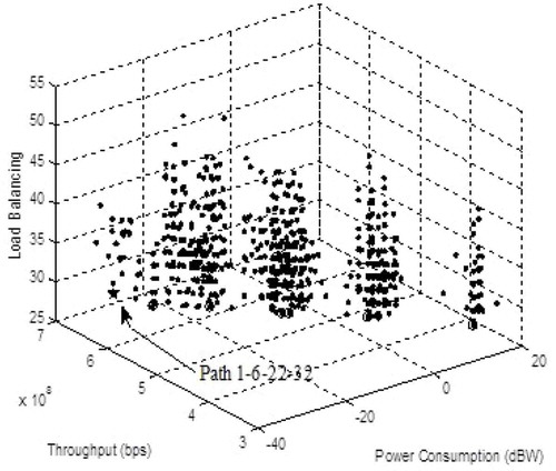
Figure 7 shows the load balancing with the smallest value of 27.7122 dB indicated bythe circle and star sign. The path for outside is selected ie (1-10-22-32) when using three criteria with the smallest Euclidean distance 0.0223 with star sign. While the indoor track is selected from 1-6-22-32 because the smallest Euclidean distance is 0.0804 with star sign. The result shows in Figure 8.

Next, the selection of a path pairs of optimal relays is based on a cross-layer optimization on multi-hop wireless ad hoc network (Gunantara & Hendrantoro, 2013a). The cross-layer performance indicators that are reviewed are power consumption, signal-to-noise ratio (SNR), and load balance. The combination of the path pairs for a number of N nodes on 3 hops and 3 hops is $(N-2)(N-3)P_2^{(N-2)-2}$ solutions.

Results for one simulation are used to find the cooperative path pair. As for the simulation conducted 500 times, it is shown in the form of the cumulative distribution function (CDF) and simulation time.

Based on the analysis of optimization results, some conclusions can be made. First, in search of a cooperative path pair based on the Pareto method, the performance indicators formed are separated. Second, the Pareto method is an approximately ideal optimization, as evidenced by the three performance indicators of ad hoc networks. Third, the required computation time is 61.1 h.

The next Pareto method application is the cooperative diversity protocol with the multi-criteria problem of SNR and load variance. Unlike the previous application where the optimal value is found by exhaustive methods, this application uses the continuously updated algorithm to obtain a non-dominated solution (Gunantara & Sastra, 2016). The advantage of this protocol is to provide the best and fairness cooperative diversity path. Based on the simulation results, the non-dominated solution as POF can be seen in Figure 9.

Figure 9. POF for SNR and load variance.

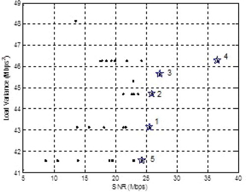
Figure 9 shows five non-dominated solutions solutions are stars sign with numbers. The 1st star shows the path (S – 11 – D) with a SNR value = 25.55 Mbps and load variance of 43,1396 Mbps2, the 2nd star shows the path (S – 28– D) with a SNR value = 24.33 Mbps and load variance of 41,58 Mbps2, the 3rd star shows the path (S – 12 – D) with aSNR value = 27.23 Mbps and load variance of 45,64 Mbps2, the 4th star shows the path(S – 20 – D) with a SNR value = 36.61 Mbps and load variance of 46.26 Mbps2, the 5th star shows the path (S – 22 – D) with a SNR value = 25.91 Mbps and load variance of 44,70 Mbps2. Selecting two non-dominated solutions as path pairs is done. The Euclidean distance values for non-dominated solutions ist star, 2nd star, 3rd star, 4th star and 5th star are 0.1087, 0.3792, 0.4251, 0.4347, and 0.4808 respectively. Therefore, the two path pairs selected based on their smallest Euclidean distance are path ((S – 11 – D)) and path ((S – 28 – 32)).

3.2. Application of scalarization method

Cross layer optimization is applied for optimal relay selection on multi-hop wireless ad-hoc network. The performance indicators reviewed are power consumption, SNR, and load balance that is optimized using the scalarization methods that give justice to every resource and are given equal weights (Gunantara & Hendrantoro, 2013a). The ad hoc network models are in two conditions, outside and inside the building. The two configurations have 32 nodes where source specified at node 1, destination is specified at node 32, and the other node acts as relay. The combination of the path pairs can be 3 hops and 3 hops of $(N-2)(N-3)P_2^{(N-2)-2}$ solutions.

The number searches of existing path pairs based on the configuration of the model affect the determination of the optimal value on the scalarization method assisted by the GA. The simulation is done once and 500 times in determining optimal cooperative path pairs. The results of the one-time simulation are used to find the cooperative path pairs, while the 500-time simulation is shown in the form of CDF and simulation time.

Some conclusions can be made based on the analysis of optimization results. First, in searching for a cooperative path pair based on the scalarization method, the performance indicator components that make up the scalar function are already incorporated into the fitness function. The scalarization method for all three performances on outdoor configurations yields a fitness value of 2.4858. The selected cooperative path pairs are 1 (1–3–22–32) and 2 (1–4–14–32). Meanwhile, the indoor configuration obtained path pairs $R1$ (1–26–6–32) and $R2$ (1–10–14–32) with a fitness value of—9.0105. Lastly, the scalarization method takes 13.96 h to complete the simulation.

The next application of the scalarization method is the creation of a simple and easy-to-understand cooperative protocol with multi-objective criterion that takes into account the *source–destination (S–D) conditions with the amplify and forward method (Gunantara et al., 2014). In addition, this cooperative diversity protocol guarantees full diversity based on three objective criteria. These criteria are SNR, power consumption, and load variance.

This protocol testing is performed on S sending data packets by broadcast to D, assisted by multi-relay of 30 nodes. The communication protocol starts from the source S sending the packet through the broadcast. The decision of a good S–D quality us determined based on the SNR value from S to D. If the SNR value from S to D is greater than two power two spectral efficiencies, then the one dual-hop procedure is selected. Meanwhile, if the SNR value from S to D is less than two power two spectral efficiency, then two dual-hop procedure is chosen. There are three possibilities of the protocol, namely diversity, no diversity, and no connection.

From the simulation result of the protocol testing, SNR value with the proposed algorithm was obtained by considering the S–D condition is bigger than the single objective algorithm, which does not consider the S–D condition. An improve in SNR was obtained at 3.06 dB. Third, the power consumption tends to be at 3 W. The proposed model ensures full diversity communication.

In contrast to the previous simulation, the selection of path pairs in this ad hoc network uses varying weights on each criterion. The large weight assigned to the criterion indicates that the criterion has a higher priority than the ones with smaller weights. The weighted approach used is RS weights for power consumption, SNR, and load variance (Gunantara and Dharma 2017).

The wireless ad hoc network that is reviewed is a configuration outside the building. Nodes are generated in open space with an area of 40 m x 40 m for outside conditions. Nodes are generated with 32 nodes in random positions. Source specified on the node 1, destination specified by node 32, and another node as relay. With a large number of path pairs and complicated computations, the method used in finding the optimal value is a GA.

From the simulation results, it shows that first, with varying weights on the function of scalarization, the optimal path pairs are chosen differently according to the resulting fitness value. Second, a weight of 0.5 has a higher priority, resulting in the greatest performance value (for the maximizing objective function) or the smallest performance value (for the minimizing objective function). Finally, the computational time required for scalarization functions with varying weights has little to no difference. The computational time difference can be seen if it is compared with the exhaustive method by checking the overall solutions. The computation time using the exhaustive process is 3.72 times longer compared to the GA optimization.

The next step is done using PSO in terms of selecting the optimal path pairs on multi-criteria ad hoc networks with varying weights (Gunantara, Sudiarta, & Antara, 2018). Furthermore, there is a comparison with the GA method that has been studied. The comparison of these two algorithms s is done because both algorithms have similarities and differences. These two metaheuristic algorithms are GA and PSO. Although the algorithm equally generates the population, the difference be-tween GA and PSO is that in GA there are crossover and mutation but in PSO there is no crossover and mutation.

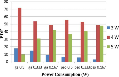
Results show that first, with varied weights, the performance of SNR with GA method is better than the PSO method. Larger weights for SNR produce better SNR performance compared to smaller weights. Larger weights mean having a higher priority. The results can been seen in Figure 10. Second, Figure 11 show that with varied weights, the performance of load variance with GA method is better than the PSO method. Larger weights for load variance produce performance of load variance is better compared to smaller weights. Third, with varied weights, the performance of power consumption with GA method is better than the PSO method. Larger weights for power consumption produce performance of power consumption is better compared to smaller weights. The results can been seen in Figure 12. Lastly, in terms of computing time, GA method takes longer computation compared to PSO method.

Figure 10. CDF of SNR.

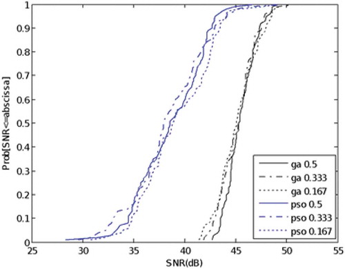
Figure 11. CDF of load variance.

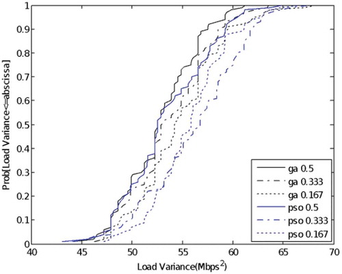
Figure 12. PDF of power consumption.

4. Conclusions

The problems in MOO are numerous and can be found in various areas of human life. Along with this, there are also many methods in solving the MOO problem. In this MOO review, there are two conclusions. Firstly, there are two MOO methods that do not require complex mathematical equations so that the problem becomes simplified, namely the Pareto and scalarization methods. In the Pareto method, there are dominated solutions and non-dominated solutions that can be described in POF. The non-dominated solution is obtained through the continuously updated algorithm. The scalarization method creates multi-objective functions into a single solution, and the weights are first determined. The weights on the scalarization method are equal weights, ROC weights, and RS weights. Second, the solution from the Pareto method is a performance indicator that forms MOO a separate and produces a compromise solution and can be displayed in the form of POF. Meanwhile, the solution with the scalarization method is in the form of performance indicators that form the scalar function that is incorporated in the fitness function.

Correction

This article has been republished with minor changes. These changes do not impact the academic content of the article.

Additional information

Funding

The research work of N. Gunantara has been supported by a Hibah Penelitian Berbasis Kompetensi 2018 Contract No: 171.30/UN14.4.A/LT/2018 from Ministries of Research, Technology and Higher Education and the United States Agency for Interna-tional Development (USAID) through the Sustainable Higher Education Research Al-liance (SHERA) Program for Universitas Indonesia's Scientic Modeling, Application,Research and Training for City-centered Innovation and Technology (SMART CITY)Project, Grant #AID-497-A-16-00004, Sub Grant #IIE-00000078-UI-1.

Notes on contributors

Nyoman Gunantara

Nyoman Gunantara, joined with Universitas Udayana (Unud), Bali as lecturer since 2001. He holds Bachelor degree in electrical engineering from Universitas Brawijaya (UB), Master and Doctor degrees in electrical engineering from Institut Teknologi Sepuluh Nopember (ITS). He has 17 years of teaching and research experience. His research interests include wireless communications, ad hoc network, quality network, and optimization. He is a member of the IEEE.

References

- J. S. Dodgson., M. Spackman., A. Pearman., & L. D. Phillips . (2009). Multi-criteria analysis: A manual . London: Department for Communities and Local Government.
- Barron, F. H. , & Barrett, B. E. (1996). Decision quality using ranked attribute weights. Management Science , 42(11), 1515–1523. doi:10.1287/mnsc.42.11.1515
- Boyd, S. , & dan Vandenberghe, L. (2004). Convex optimization . Cambridge University Press.
- Chang, C. T. (2007). Multi-choice goal programming. Omega , 35(4), 389–396. doi:10.1016/j.omega.2005.07.009
- Charnes, A. , Clower, R. W. , & Kortanek, K. O. (1967). Effective control through coherent decentralization with preemptive goals. Econometrica , 35, 294–320. doi:10.2307/1909114
- Charnes, A. , & Cooper, W. W. (1961). Management models and industrial applications of linear programming . New York: John Wiley and Sons.
- Charnes, A. , Cooper, W. W. , & Ferguson, R. O. (1955). Optimal estimation of executive compensation by linear programming. Management Science , 1, 138–151. doi:10.1287/mnsc.1.2.138
- Chong, E. K. P. , & Zak, S. H. (2008). An introduction to optimization (3rd ed.). USA: John Wiley and Sons.
- Cohanim, B. E. , Hewitt, J. N. , & de Weck, O. (2004). The design of radio telescope array configurations using multiobjective optimization: Imaging performance versus cable length. The Astrophysical Journal Supplement Series , 154(2), 705–719. doi:10.1086/apjs.2004.154.issue-2
- Cohon, J. L. (1983). Multi-objective programming and planning . New York: Academic Press.
- Das, I. , & Dennis, J. E. (1997). A closer look at drawbacks of minimizing weighted sums of objectives for Pareto set generation in multi-criteria optimization problems. Structural Optimization , 14, 63–69. doi:10.1007/BF01197559
- Dawes, R. M. , & dan Corrigan, B. (1974). Linear models in decision making. Psychological Bulletin , 81, 95–106. doi:10.1037/h0037613
- Deb, K. (2001). Multi-objective optimization using evolutionary algorithms . England: John Wiley and Sons.
- Deb, K. , & Datta, R. (2012). Hybrid evolutionary multi-objective optimization and analysis of machining operations. Engineering Optimization , 44(6), 685–706. doi:10.1080/0305215X.2011.604316
- Ehrgott, M. (2005). Multicriteria optimization . Germany: Springer.
- Einhorn, H. J. , & McCoach, W. (1977). A simple multiattribute utility procedure for evaluation. Behavioral Science , 22(4). doi:10.1002/bs.3830220405
- Fishburn, P. C. (1974). Lexicographic orders, utilities, and decision rules: A survey. Management Science , 20(11), 1442–1471. doi:10.1287/mnsc.20.11.1442
- Gunantara, N. , & Dharma, A. (2017, April). Optimal path pair routes through multi-criteria weights in ad hoc network using genetic algorithm. International Journal of Communication Networks and Information Security (IJCNIS) , 9(1).
- Gunantara, N. , & Hendrantoro, G. (2013a). Multi-objective cross layer optimization for selection of cooperative path pairs in multihop wireless ad hoc networks. Journal of Communications Software and Systems , 9(3), 170. doi:10.24138/jcomss.v9i3.146
- Gunantara, N. , & Hendrantoro, G. (2013b). Multi-objective cross-layer optimization with Pareto method for relay selection in multihop wireless ad hoc networks. WSEAS Transaction on Communications , 12(3).
- Gunantara, N. , & Sastra, N. P. (2016). Cooperative diversity selection protocol using Pareto method with multi objective criterion in wireless ad hoc networks. International Journal of Multimedia and Ubiquitous Engineering , 11(5), 43–54. doi:10.14257/ijmue
- Gunantara, N. , Sastra, N. P. , & Hendrantoro, G. (2014). Cooperative diversity path pairs selection protocol with multi objective criterion in wireless ad hoc networks. International Journal of Applied Engineering Research , 9(23).
- Gunantara, N. , Sudiarta, P. K. , & Antara, I. N. G. (2018). Multi-criteria weights on ad Hoc networks using particle swarm optimization for optimal path pairs. International Review of Electrical Engineering (IREE) , 13(1), 15. doi:10.15866/iree.v13i1.14082
- Gunasekara, R. C. , Mehrotra, K. , & Mohan, C. K. (2014, August 17–20). Multi-objective optimization to identify key players in social networks . IEEE/ACM international conference on Advances in Social Networks Analysis and Mining (ASONAM).
- Haimes, Y. Y. , Lasdon, S. , & Wismer, D. A. (1971). On a bicriteriion formulation of the problem of integrated system identification and system optimization. IEEE Transactions on Systems, Man, and Cybernetics , 1(3), 296–297.
- Hokey, M. , & James, S. (1991). On the origin and persistence of misconceptions in goal programming. Journal of Operational Research Society , 42(4), 301–312. doi:10.1057/jors.1991.68
- Horn, J. , Nafpliotis, N. , & Goldberg, D. E. (1994, June). A niched Pareto genetic algorithm for multiobjective optimization. In Proceedings of the first IEEE conference on evolutionary computation, IEEE world congress on computational intelligence (Vol. 1, pp. 8287). Piscataway, NJ: IEEE Service Center.
- Ignizio, J. P. (1974). Generalized goal programming: An overview. Computer and Operations Research , 10(4), 277–289. doi:10.1016/0305-0548(83)90003-5
- Jena, S. (2013). Multi-objective optimization of the design parameters of shell and tube type heat exchanger based on economic and size consideration ( A Thesis Bachelor of Technology in Mechanical Engineering). National Institute of Technology, Rourkela.
- Jia, J. , Fischer, G. W. , & Dyer, J. S. (1998). Attribute weighting methods and decision quality in the presence of response error: A simulation study. Journal of Behavioral Decision Making , 11(2), 85–105. doi:10.1002/(ISSN)1099-0771
- Kim, I. Y. , & de Weck, O. L. (2005). Adaptive weighted sum method for bi-objective optimization: Pareto front generation. Structural Multidisciplinary Optimization , 29, 149–158. doi:10.1007/s00158-004-0465-1
- Lam, T. B. , & Sameer, A. (2008). Multi-objective optimization in computational intelligence: Theory and practice . USA: Information Science Reference.
- Mardle, S. , Pascoe, S. , & Tamiz, M. (1998). An investigation of genetic algorithms for the optimization of multiobjective fisheries bioeconomic models. In Proceeding of the third international conference on multi-objective programming and goal programming: Theory and applications (MOPGP98) . Quebec City.
- Messac, A. , Sukam, C. P. , & Melachrinoudis, E. (2000a). Aggregate objective functions and Pareto frontiers: Required relationships and practical implications. Journal of Optimization English , 1, 171–188. doi:10.1023/A:1010035730904
- Messac, A. , Sundararaj, G. J. , Tappeta, R. V. , & Renaud, J. E. (2000b). Ability of objective functions to generate points on nonconvex Pareto Frontiers. AIAA Journal , 38, 1084–1091. doi:10.2514/2.1071
- Miettinen, K. (1999). Nonlinear multiobjective optimization . Boston: Kluwer Academic Publishers.
- Murata, T. , & Ishibuchi, H. (1996). Multi-objective genetic algorithm and its application to flow-shop scheduling. International Journal of Computers and Engineering , 30(4).
- Odu, G. O. , & Charles-Owaba, O. E. (2013). Review of multi-criteria optimization methods theory and applications. IOSR Journal of Engineering (IOSRJEN) , 3(10).
- Ozcelebi, T. (2006). Multi-objective optimization for video streaming ( Ph.D Thesis). Graduate School of Sciences and Engineering, Koc University.
- Pernodet, F. , Lahmidi, H. , & Michel, P. (2009). Use of genetic algorithms for multicriteria optimization of building refurbishment . Eleventh international IBPSA conference, Glasgow, Scotland.
- Ruspini, E. H. , & Zwir, I. S. (1999). Automated qualitative description of measurements. In Proceedings of the 16th IEEE instrumentation and measurement technology conference . Venice, Italy.
- Sessarego, M. , Dixon, K. R. , Rival, D. E. , & Wood, D. H. (2015). A hybrid multi-objective evolutionary algorithm for wind-turbine blade optimization. Engineering Optimization , 47(8), 1043–1062. doi:10.1080/0305215X.2014.941532
- Steuer, R. E. (1986). Multiple criteria optimization: Theory, computation, and applications . John Wiley and Sons, Inc.
- Tapia, M. G. C. , & Coello, C. A. C. (2007, September 25–28). Applications of multi-objective evolutionary algorithms in economics and finance: A survey . IEEE Congress on Evolutionary Computation. CEC, Singapore.
- Triantaphyllou, B. , Shu, S. , Sanchez, N. , & Ray, T. (1998). Multi-criteria decision making: An operations research approach. In J. G. Webster (Ed.), Encyclopedia of electrical and electronics engineering (Vol. 15, pp. 175–186). New York, NY: John Wiley and Sons.
- Weck, O. L. D. (2004). Multiobjective optimization: History and promise. In Proceedings of 3rd China-Japan-Korea joint symposium on optimization of structural and mechanical systems . Kanazawa, Japan.
- Zeleny, M. (1973). Multiple criteria decision making. Compromise programming (pp. 262–301). University of South Carolina Press.
- Zwir, I. S. , & Ruspini, E. H. (1999). Qualitative object description: Initial reports of the exploration of the frontier. In Proceedings of the Joint EUROFUSE-SIC99 international conference . Budapest.