Construction new rational cubic spline with application in shape preservations

Abstract

This study considers the construction a new C ¹ rational cubic spline (cubic numerator and quadratic denominator) with three parameters. Some mathematical properties of this rational function will be investigated in details. In order to use the proposed rational cubic spline for positivity preserving interpolation and constrained data that lie above any arbitrary straight line, the automatic choice of one parameter will be developed through some mathematical derivation. On each sub-interval this idea gives extra two free parameters that very useful for the user to manipulate the shape of the curve while at the same time maintaining the shape preservations of the data. Numerical comparison with some existing schemes shows that, the proposed scheme is on par. Furthermore, for some data sets, the proposed scheme is better as well as produce more visually pleasing interpolating curve for scientific visualization.

Keywords:

• rational cubic spline
• positivity
• constraint line
• continuity
• interpolation

Subjects Classifications:

• 68U05
• 65D05
• 65D07
• 65D18

PUBLIC INTEREST STATEMENT

This study considers the construction a new C ¹ rational cubic spline (cubic numerator and quadratic denominator) with three parameters. The proposed rational cubic spline is implemented for positivity preserving interpolation and constrained data that lie above any arbitrary straight line. This is achieved by finding the sufficient condition that will give the automatic choice of one parameter with two free parameters for shape modification while at the same time maintaining the shape preservation. Numerical comparison with some existing schemes shows that, the proposed scheme is on par where for some data sets, the proposed scheme is better as well as produce more visually pleasing interpolating curve for scientific visualization.

The presented scheme is useful in advancing the study in image interpolation and image compression by controlling the free parameters. Furthermore, for non-technical readers, the proposed scheme also applicable for the animation industry and we believe that it is better than the common cubic Bezier and cubic spline.

1. Introduction

When the experiments are conducted in the laboratory, usually the scientists will obtain a lot of raw data that represents the results for that experiment. For instance, in chemical experiment, the data might be distillation curve or in biochemistry, the data maybe the movement of the respective cell inside the system. Furthermore, in any experiments, there must be exists the error or noise in the data acquisition processes. The error can be either systematic or bias error or random error. These data are subject for other data processing techniques such as data fitting and data smoothing or filtering. If the data is clean i.e. most probably no error, then interpolation is a better option to the data. But if the data consist error or noise, the approximation and smoothing or denoizing might be useful for the purposes. The common methods for data processing are linear regression, polynomial regression (or fitting), any non-polynomial fitting, cubic spline, smoothing spline, etc. Besides that, recently, the approximation or interpolation of the data does require that the curve or surface must be also maintain the geometric shape of the data. For instance, the positive data is given, then the curve should be positive everywhere. Furthermore, if the data lie above an arbitrary straight line, then the resulting interpolating curve must lie above a straight line. Both geometric properties are important in the field of scientific visualization, since if we consider the probability of some measurements, then the negativity is clearly meaningless. Furthermore, the level of oxygen in the gas discharge is also a positive data (Brodlie, Asim, & Unsworth, 2005).

We divided the literature review into two parts i.e. positivity preserving interpolation and constrained data modelling, respectively. Many researchers have investigated positivity preserving interpolation by using polynomial cubic spline, rational splines or the trigonometric spline. For instance, Abbas, Majid, M.N. Hj, and Ali (2012) have considered the constrained data interpolation for data lies above a straight line for curve and above a plane for surface interpolation. Their scheme has two free parameters that can be used to change the shape of the curve. Butt and Brodlie (1993) discussed positivity preserving interpolation by extending the main idea from Fritsch and Carlson (1980). Butt and Brodlie’s scheme requires the modification of the first derivatives as well as knots insertion on some sub-intervals in which the shape violation are found. Brodlie et al. (2005) discussed the positivity preserving approximation and constrained data modelling by using Shepard’s family i.e. meshfree methods. To achieve shape preserving, some optimization problem need to be solved in order to find suitable parameters. Hussain and Ali (2006) constructed positive curve by using rational cubic spline with two parameters. This idea has been extended by Hussain and Hussain (2006) for positivity preserving interpolation and constrained interpolation (both for curve and surface, respectively). The main drawback for the schemes of Hussain and Ali (2006) and Hussain and Hussain (2006) are that both schemes have no free parameters to modify the shape of the curve, since the sufficient conditions are derived on all parameters that exists in the description of their rational cubic spline. Hussain, Hussain, and Samreen (2008) implement rational quartic spline for positive and convex shape preserving interpolation. But based on our simulation, their scheme fails to preserves positivity of the data. Hussain and Sarfraz (2008) consider the positivity shape preserving by using rational cubic spline of the form cubic/cubic with two free parameters. They obtain positive interpolating curve and surface. But for some data sets, the surface tends to be flat on some region. Karim and Kong (2014) have constructed another version of rational cubic spline (cubic/quadratic) with two free parameters in each sub-interval that can be used to modify the shape of the curve. They show that their results are more visually pleasing than the scheme presented by Hussain and Hussain (2006) and Hussain et al. (2008). Sarfraz (2002) has studied the positivity preserving but his scheme has no free parameter to refine the final curve. Sarfraz, Hussain, and Chaudary (2005) discussed shape preservations by using cubic spline interpolation with $G{C}^1$ (first order of geometric continuity). It can be proved that their scheme does not guarantee to produce interpolating curve that lie above the given constraint line. Since for some data sets, the curve may violate the shape preservation requirement. The rational cubic spline scheme by Sarfraz, Hussain, and Nisar (2010) may produce negative curve on some interval that will destroys the positivity of the data. Wu, Zhang, and Peng (2010) proposed rational quartic spline for positivity preserving interpolation. Their scheme gives visually pleasing results but at a cost, the construction of the rational quartic spline is very complicated and not easy to used. Besides the use of cubic spline and various types of rational spline, recently there are some studies on the application of trigonometric spline (rational or non-rational) for shape preserving interpolation. For instance, Bashir and Ali (2013) constructed trigonometric spline for positive and constraint interpolation. Hussain, Hussain, and Waseem (2014), Ibraheem, Hussain, Hussain, and Bhatti (2012) and Liu, Che, and Zhu (2015) also consider various types of shape preservations by using difference sets of spline in trigonometric form. Liu et al. (2015) is the best scheme compare with Bashir and Ali (2013), Hussain et al. (2014) and Ibraheem et al. (2012). Since the introduction of cubic Ball in CAGD, there exist some applications in shape preserving interpolation. Karim (2013, 2015a, 2016a, 2016b, 2015b) discussed various types of rational cubic Ball for shape preserving interpolation. The main objective of this study is to overcome the drawback in the schemes of Fritsch and Carlson (1980)-PCHIP in MATLAB, Butt and Brodlie (1993), Brodlie et al. (2005), Hussain et al. (2008; Hussain, Sarfraz, & Shaikh, 2011), Hussain and Ali (2006) and Sarfraz et al. (2005, 2010). To meet the objective, we propose new rational cubic spline (cubic/quadratic) with three parameters. We identify few advantages of the proposed schemes compare with other schemes such as:

1. The proposed scheme is free from first derivative modification for shape preservations. The schemes of Butt and Brodlie (1993) and Fritsch and Carlson (1980) do required some derivative modification.

2. The proposed scheme is guarantee to produce positive interpolating curve everywhere. Meanwhile in the schemes proposed by Hussain et al. (2008) and Hussain et al. (2011) and Sarfraz et al. (2010), positivity might not be preserved on some sub-intervals such that along the whole interval, the function value is negative i.e. lie below x-axis.

3. For constrained data interpolation, the proposed scheme produces interpolating curve that lie above a straight line, but the scheme of Sarfraz et al. (2005) give some interpolating curve that lies below a straight line. Comparing with Karim and Kong (2014), the proposed scheme gives more visually pleasing interpolating curve as well as the curve is very closed to the constraint line.

This paper is organized as follows. Section 2 presents the methodology of the proposed study. This includes the construction of another version of rational spline with quadratic denominators where in each sub-interval; it has three parameters, derivative estimation and geometric properties of the rational interpolant. Shape control analysis will be shown with numerical examples. Section 3 describes about the shape preserving interpolation applications. We consider positivity preserving and constrained data modelling. The automated choice of one parameter that will ensure the rational interpolant satisfies shape preservations properties will be derived with two parameters to refine the curve shape. Section 4 presents the numerical and graphical results, including comparison with established schemes. Finally, Section 5 concludes the paper and presents future recommendation studies by using the proposed scheme.

2. Methodology of the study

We begin with the construction of new rational spline $S\left(x\right)$ (cubic numerator and quadratic denominator) with three parameters ${\alpha }_i,{\beta }_i$, and ${\gamma }_i$, for $i=0,1,\dots ,n-1$. This section is divided into few subsection as follows: the construction of new rational cubic spline, derivative estimation and the geometric properties of the proposed rational interpolant.

2.1. Rational spline construction

Given data $\left\{\left(x_i,f_i\right),i=0,1,\dots ,n\right\}$ where $x_0<x_1<\cdots <x_n$ and the first derivatives $d_i,\hspace{0.17em}i=0,1,\dots ,n$. Let, ${\mathrm{\Delta }}_i=\left(f_{i+1}-f_i\right)/h_i$ and $\theta =\left(x-x_i\right)/h_i$ such that when $x=x_i$ then $\theta =0$ and similarly when $x=x_{i+1}$ then $\theta =1$. Thus $0\le \theta \le 1$. For $x\in \left[x_i,x_{i+1}\right],i=0,1,\dots ,n-1$, the rational cubic spline with three parameters ${\alpha }_i,{\beta }_i$, and ${\gamma }_i$, for $i=0,1,\dots ,n-1$ is defined by

(1) $S\left(x\right)=S_i\left(x\right)=\frac{P_i\left(\theta \right)}{Q_i\left(\theta \right)},$(1)

where

$P_i\left(\theta \right)={\left(1-\theta \right)}^3{A}_I+{\left(1-\theta \right)}^2\theta B_i+\left(1-\theta \right){\theta }^2{C}_i+{\theta }^3{E}_i$

$Q_i\left(\theta \right)={\alpha }_i{\left(1-\theta \right)}^2+\left({\alpha }_i+{\gamma }_i\right)\left(1-\theta \right)\theta +{\beta }_i{\theta }^2$

The common requirement for the parametric continuity is $C^1$ or $C^2$ continuous. Throughout this study, we only consider the construction of rational cubic spline with $C^1$ continuity. This condition can be described as follows (Fritsch & Carlson, 1980; Sarfraz, 2002):

(2) $\begin{array}{cc}S\left(x_i\right)=f_i,& S^{\left(1\right)}\left(x_i\right)=d_i\\ \\ S\left(x_{i+1}\right)=f_{i+1},& S^{\left(1\right)}\left(x_{i+1}\right)=d_{i+1}\end{array}$(2)

By applying Condition (2) to Equation (1), we obtain the unknown $A_i,B_i,C_i$ and $E_i$ for $i=0,1,\dots ,n-1$ as follows:

$\begin{array}{c}{A}_i={\alpha }_i{f}_i,\hspace{0.17em}{B}_i=\left(2{\alpha }_i+{\gamma }_i\right)f_i+{\alpha }_i{h}_i{d}_i,\hspace{0.17em}\\ {\mathrm{C}}_i=\left({\alpha }_i+{\beta }_i+{\gamma }_i\right)f_{i+1}-{\beta }_i{h}_i{d}_{i+1},{\mathrm{E}}_i={\beta }_i{f}_{i+1}\hspace{0.17em}\end{array}$

Therefore, the rational cubic spline in (1) can be written as

(3) $S\left(x\right)=\frac{{\left(1-\theta \right)}^3{\alpha }_i{f}_i+{\left(1-\theta \right)}^2\theta \left(\left(2{\alpha }_i+{\gamma }_i\right)f_i+{\alpha }_i{h}_i{d}_i\right)+\left(1-\theta \right){\theta }^2\left(\left({\alpha }_i+{\beta }_i+{\gamma }_i\right)f_{i+1}-{\beta }_i{h}_i{d}_{i+1}\right)+{\theta }^3{\beta }_i{f}_{i+1}}{{\alpha }_i{\left(1-\theta \right)}^2+\left({\alpha }_i+{\gamma }_i\right)\left(1-\theta \right)\theta +{\beta }_i{\theta }^2}$(3)

2.2. Derivative estimation

There exist various methods that can be used to estimate the first derivative $d_i,i=0,1,\dots ,n$ such as geometric mean method (GMM), harmonic mean method (HMM) and arithmetic mean method (AMM). Since AMM is simple and easy to use as well as suitable for all types of data sets (Hussain & Sarfraz, 2008), throughout this study we utilized AMM. Its formulation is given below:

For $i=1,2,3,\dots ,n-1$, $d_i$ is calculated as follows (Sarfraz, 2002):

(4) $d_i=\frac{h_{i-1}{\mathrm{\Delta }}_i+h_i{\mathrm{\Delta }}_{i-1}}{h_{i-1}+h_i},$(4)

Meanwhile, at $i=0$ and $i=n$, the derivative value of $d_0$ and $d_n$ are given as

(5) $d_0={\mathrm{\Delta }}_0+\left({\mathrm{\Delta }}_0-{\mathrm{\Delta }}_1\right)\left(\frac{h_0}{h_0+h_1}\right)$(5)

(6) $d_n={\mathrm{\Delta }}_{n-1}+\left({\mathrm{\Delta }}_{n-1}-{\mathrm{\Delta }}_{n-2}\right)\left(\frac{h_{n-1}}{h_{n-1}+h_{n-2}}\right)$(6)

Furthermore, if the data are equally space, then for $i=1,2,3,\dots ,n-1$, the first derivatives are given as

$d_i=\frac{{\mathrm{\Delta }}_i+{\mathrm{\Delta }}_{i-1}}{2}.$

2.3. Geometric properties of the rational spline

The geometric properties of the proposed rational cubic spline defined by (3) are investigated in this section. The main focus is on the shape control analysis of the rational spline. This shape control in important in order for us to determine the condition on ${\alpha }_i,{\beta }_i$, and ${\gamma }_i$, for $i=0,1,\dots ,n-1$. Furthermore, we will see various types of interpolating curves corresponding with various value of parameters ${\alpha }_i,{\beta }_i$, and ${\gamma }_i$. There are three geometric properties that can be observed:

• If ${\alpha }_i={\beta }_i={\gamma }_i=1$, the rational spline interpolant defined by (3) is reduce to cubic Hermite spline polynomial that can be expressed as

(7) $S_i\left(x\right)=f_i{\left(1-\theta \right)}^3+\left(3f_i+h_i{d}_i\right){\left(1-\theta \right)}^2\theta +\left(3f_{i+1}-h_i{d}_{i+1}\right){\left(1-\theta \right)}^2\theta +f_{i+1}{\theta }^3$(7)

which can be simplified to

$S_i\left(x\right)=f_i{\left(1-\theta \right)}^2\left(1+2\theta \right)+h_i{d}_i{\left(1-\theta \right)}^2\theta -h_i{d}_{i+1}{\left(1-\theta \right)}^2\theta +f_{i+1}{\theta }^2\left(3-2\theta \right)$

• After some derivation and simplification, the piecewise rational cubic spline $S_i\left(x\right)$ defined by (3) can be written as

(8) $S_i\left(x\right)=\left(1-\theta \right)f_i+\theta f_{i+1}+\frac{h_i\left(1-\theta \right)\theta \left[{\alpha }_i\left(d_i-{\mathrm{\Delta }}_i\right)\left(1-\theta \right)+{\beta }_i\left({\mathrm{\Delta }}_i-d_{i+1}\right)\theta \right]}{{\alpha }_i{\left(1-\theta \right)}^2+\left({\alpha }_i+{\gamma }_i\right)\left(1-\theta \right)\theta +{\beta }_i{\theta }^2}$(8)

From (8), when ${\gamma }_i\to \mathrm{\infty }$, the rational cubic interpolant $S_i\left(x\right)$ reduce to a straight line on each sub-interval $\left[x_i,x_{i+1}\right],$for $i=0,1,...,n-1$. This is also applicable when ${\alpha }_i,{\beta }_i\to 0$. Thus the following limit is obtained:

(9) $\underset{{\alpha }_i,{\beta }_i\to 0,{\gamma }_i\to \mathrm{\infty }}{lim{S}_i\left(x\right)}=\left(1-\theta \right)f_i+\theta f_{i+1}$(9)

• When ${\alpha }_i<0$, or ${\beta }_i<0$ or ${\gamma }_i\le -3$, the rational cubic spline interpolant defined by (3) turn to be the standard rational function with vertical asymptotes or poles on sub-interval $\left[x_i,x_{i+1}\right],i=0,1,\dots ,n-1$.

A positive data set taken from Wu et al. (2010) is shown in Table 1. The data sets show the velocity of the wind that has the positive values.

Table 1. A wind data

$i$	0	1	2	3	4	5	6
$x_i$	0	0.25	0.5	1	1.2	1.8	2
$f_i$	2	0.8	0.5	0.1	1	0.5	1
$d_i$	−6.6	−3	−1.067	2.986	3.167	1.667	3.333

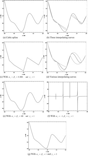
Figure 1 shows the examples of shape control properties. Figure 1(a) shows the cubic Hermite when ${\alpha }_i={\beta }_i={\gamma }_i=1$. Figure 1(b) shows the effect when we increases the value of one parameter i.e. ${\gamma }_i$ while ${\alpha }_i={\beta }_i=1$:${\gamma }_i=1$ (solid), ${\gamma }_i=10$ (dashed) and (grey). Clearly as${\gamma }_i\to \mathrm{\infty }$, the rational cubic spline approaching a straight line on each sub-interval. Figure 1(c) also shows the effect that the rational cubic spline reduces to a straight line when both ${\alpha }_i,{\beta }_i\to 0$. Figure 1(d) shows the effect when ${\alpha }_i={\beta }_i=1$:${\gamma }_i=1$ (solid), ${\alpha }_i=0,{\beta }_i={\gamma }_i=1$(dashed) and ${\beta }_i=0,{\alpha }_i={\gamma }_i=1$(gray). Figure 1(e) shows that when both ${\alpha }_i,{\beta }_i\to \mathrm{\infty }$, the rational spline does not reduce to a straight line. Figure 1(f) shows that the interpolating curve have poles when ${\alpha }_i=-1,{\beta }_i={\gamma }_i=1$. This is also true when ${\beta }_i<0$ or ${\gamma }_i\le -3$. This is the main reason that, the parameters are chosen such that ${\alpha }_i,{\beta }_i>0$, and ${\gamma }_i\ge 0$ for $i=0,1,\dots ,n-1$. Finally Figure 1(g) shows the effect when ${\alpha }_i={\beta }_i=1$ and ${\gamma }_i=5$. From this graph, the positivity of the data set is preserved and it is visually pleasing.

Figure 1. Various types of interpolating curves based on shape control analysis.

3. Shape preservations

In this section, we derive the sufficient condition for the positivity of the proposed rational cubic spline on one parameter. We begin with positivity preserving interpolation and the idea for positivity preserving is extended to constrained data interpolation for data that lie above an arbitrary straight line.

3.1. Positivity preserving

In order to avoid divided by zero later, we assume that, the given data is strictly positive

(10a) $f_i>0,\hspace{0.17em}i=0,1,2,\dots ,n$(10a)

The main objective is to find the condition on ${\gamma }_i>0$, $i=0,1,\dots ,n-1$ that will ensure the rational spline defined by (3) is positive everywhere. Mathematically, this statement can be expressed as

(10b) $S_i\left(x\right)>0,\hspace{0.17em}i=0,1,2,\dots ,n-1$(10b)

We can preserve the positivity by manipulating the value of the parameters ${\alpha }_i,{\beta }_i>0$, and ${\gamma }_i\ge 0$, for$i=0,1,2,\dots ,n-1$ (see Figure 1(g), the positivity of the data in Table 1 is preserved when ${\alpha }_i={\beta }_i=1$ and ${\gamma }_i=5$, etc.). But this approach is not practical and really time consuming to find suitable value for all parameters. Our aim is to find the automated choice on one parameter ${\gamma }_i>0$, $i=0,1,\dots ,n-1$ that will produce positive rational cubic interpolant that resulting the positive interpolating curve on the whole given domain (by satisfying Condition (10b)). Meanwhile, ${\alpha }_i,{\beta }_i>0$ are free parameters for shape modification. For ${\alpha }_i,{\beta }_i>0$, and ${\gamma }_i\ge 0$ for $i=0,1,\dots ,n-1$, the denominator $Q_i\left(\theta \right)$ is positive i.e. $Q_i\left(\theta \right)>0$. Therefore, the sufficient condition for the positivity of the rational interpolant defined by (3) can be derived by considering only the numerator i.e. the cubic polynomial $P_i\left(\theta \right),i=0,1,\dots ,n-1$ such that $P_i\left(\theta \right)>0$. Therefore, the rational cubic spline $S_i\left(x\right)>0,\hspace{0.17em}$if the cubic polynomial $P_i\left(\theta \right)>0$ for $i=0,1,2,\dots ,n-1$. The following results are obtained by Schmidt and Hess (1988). The cubic spline $P_i\left(\theta \right),i=0,1,\dots ,n-1$ is positive if

(11) $\left({P^{\prime }}_i\left(0\right),{P^{\prime }}_i\left(1\right)\right)\in R_1\cup R_2$(11)

where

(12) $R_1=\left\{\left(a,b\right):a>\frac{-3P_i\left(0\right)}{h_i},b<\frac{3P_i\left(1\right)}{h_i}\right\}$(12)

(13) $R_2=\left\{\begin{array}{c}\left(a,b\right):36f_i{f}_{i+1}\left(a^2+b^2+ab-3{\mathrm{\Delta }}_i\left(a+b\right)+3{\mathrm{\Delta }}_i^2\right)+\\ \\ 3\left(f_{i+1}a-f_{i}b\right)\left(2h_{i}ab-3f_{i+1}a+3f_{i}b\right)+4h_i\left(f_{i+1}{a}^3-f_i{b}^3\right)-h_i^2{a}^2{b}^2>0\end{array}\right\}.$(13)

Note: Here $a=P_i^{\prime }\left(0\right)$ and $b=P_i^{\prime }\left(1\right)$, respectively.

The sufficient condition for the positivity of $S_i\left(x\right),\hspace{0.17em}i=0,1,2,\dots ,n-1$ can be derived either by using (12) or (13). But since Condition (12) is simple to be used compared to (13) and this condition also will guarantee to produce the positive cubic polynomial everywhere. Therefore, in this study we will use Condition (12). This condition has been used by many other authors (Hussain & Ali, 2006; Hussain & Hussain, 2006; Hussain et al., 2014; Hussain & Sarfraz, 2008; Hussain et al., 2011; Ibraheem et al., 2012; Karim, 2013, 2015a, 2016a, 2016b, 2015b; Karim & Kong, 2014; Liu et al., 2015; Sarfraz, 2002; Sarfraz et al., 2005, 2010).

The following theorem gives the sufficient conditions for the positivity of rational spline.

Theorem 1. Given strictly positive data in (10a), rational cubic interpolant $S\left(x\right)$ defined by (3) is positive everywhere if in each sub-interval $\left[x_i,x_{i+1}\right],i=0,1,\dots ,n-1$, the parameter ${\gamma }_i>0$, $i=0,1,\dots ,n-1$ satisfies the following condition:

${\alpha }_i,{\beta }_i>0,$

(14) ${\gamma }_i>\mathrm{M}\mathrm{a}\mathrm{x}\left\{0,-{\alpha }_i\left(\frac{h_i{d}_i}{f_i}+2\right),{\beta }_i\left(\frac{h_i{d}_{i+1}}{f_{i+1}}-1\right)-{\alpha }_i\right\}$(14)

Proof.

Firstly, we derive the first derivative of $P_i^{\prime }\left(\theta \right)$ which can be written as

$P_i^{\prime }\left(\theta \right)=\frac{-3{\alpha }_i{f}_i{\left(1-\theta \right)}^2+B_i\left({\left(1-\theta \right)}^2-2\theta \left(1-\theta \right)\right)+C_i\left(-{\theta }^2+2\theta \left(1-\theta \right)\right)+3{\beta }_i{f}_{i+1}{\theta }^2}{h_i}$

where

$\begin{array}{c}{B}_i=\left(2{\alpha }_i+{\gamma }_i\right)f_i+{\alpha }_i{h}_i{d}_i,\hspace{0.17em}\\ {\mathrm{C}}_i=\left({\alpha }_i+{\beta }_i+{\gamma }_i\right)f_{i+1}-{\beta }_i{h}_i{d}_{i+1}\hspace{0.17em}\end{array}$

The sufficient condition of the positivity is derived by using (12):

(15) $P_i^{\prime }\left(0\right)>\frac{-3P_i\left(0\right)}{h_i}\Rightarrow \frac{-3{\alpha }_i{f}_i+\left(2{\alpha }_i+{\gamma }_i\right)f_i+{\alpha }_i{h}_i{d_i}_{\mathrm{i}}}{h_i}>\frac{-3{\alpha }_i{f}_i}{h_i}$(15)

and

(16) $P_i^{\prime }\left(1\right)<\frac{3P_i\left(1\right)}{h_i}\Rightarrow \frac{3{\beta }_i{f}_{i+1}-\left({\alpha }_i+{\beta }_i+{\gamma }_i\right)f_{i+1}+{\beta }_i{h}_i{d_{i+1}}_{\mathrm{i}}}{h_i}<\frac{3{\beta }_i{f}_{i+1}}{h_i}$(16)

Both conditions can be further simplified to

(17) ${\gamma }_i>-{\alpha }_i\left(\frac{h_i{d}_i}{f_i}+2\right)$(17)

and

(18) ${\gamma }_i>{\beta }_i\left(\frac{h_i{d}_{i+1}}{f_{i+1}}-1\right)-{\alpha }_i$(18)

By using (17) and (18), $S_i\left(x\right)>0,\hspace{0.17em}i=0,1,2,\dots ,n-1$ if parameter ${\gamma }_i>0$, $i=0,1,\dots ,n-1$ satisfy the following positivity condition:

${\gamma }_i>\mathrm{M}\mathrm{a}\mathrm{x}\left\{0,-{\alpha }_i\left(\frac{h_i{d}_i}{f_i}+2\right),{\beta }_i\left(\frac{h_i{d}_{i+1}}{f_{i+1}}-1\right)-{\alpha }_i\right\},\hspace{0.17em}i=0,1,\dots ,n-1$

This condition can be written as

(19) ${\gamma }_i={\epsilon }_{\mathrm{i}}+\mathrm{M}\mathrm{a}\mathrm{x}\left\{0,-{\alpha }_i\left(\frac{h_i{d}_i}{f_i}+2\right),{\beta }_i\left(\frac{h_i{d}_{i+1}}{f_{i+1}}-1\right)-{\alpha }_i\right\},\hspace{0.17em}i=0,1,\dots ,n-1$(19)

such that $0<{\epsilon }_i\le 0.5$.

The following is an algorithm for computer implementation.

Algorithm 1: positivity preserving interpolation

Input: Data points, first derivative and the parameters ${\alpha }_i,{\beta }_i>0$ and ${\epsilon }_i>0$.

Output: positive interpolating curve

Step 1: Input data points $\left\{\left(x_i,f_i\right),i=0,1,2,\dots ,n\right\}$

Step 2: For $i=1,\dots ,n$

• Calculate the first derivative values by using AMM.

Step 3: For $i=1,\dots ,n-1$

• Input parameters ${\alpha }_i,{\beta }_i>0$ and ${\epsilon }_i>0$.

• Calculate the parameter values, ${\gamma }_i>0$ by using the sufficient condition (19).

• Repeat by choosing different value of ${\alpha }_i,{\beta }_i>0$ and ${\epsilon }_i>0$.

Step 4: For $i=1,\dots ,n-1$

• Construct positive curve with $C^1$ continuity using rational cubic spline defined by (3).

3.2. Constrained data interpolation

The constrained data interpolation for data that lie on a same side as the constraint line is constructed by extending the positivity scheme discussed in the previous section. In this study, we only consider the data that lie above straight line. The problem statement can be read as follows:

Given positive data set $\left\{\left(x_i,f_i\right),i=0,1,\dots ,n\right\}$ lie above a straight line $y=mx+c$ such that

(20) $f_i>m{x}_i+c,i=0,1,\dots ,n.$(20)

The rational spline interpolation $S_i\left(x\right)$ defined in (3) lie above a straight line $\left(1-\theta \right)a_i+\theta b_i,i=0,1,\dots ,n-1$ if

(21) $S_i\left(x\right)>a_i\left(1-\theta \right)+b_i\theta$(21)

Here, we adopted the notation $a_i=m{x}_i+c,$ $i=0,1,\dots ,n$ and $b_i=m{x}_{i+1}+c,$ $i=0,1,\dots ,n-1$.

(21) $\mathrm{O}\mathrm{n}\left[x_i,x_{i+1}\right],i=0,1,\dots ,n-1,from$(21)

(22) $S_i\left(x\right)=\frac{P_i\left(\theta \right)}{Q_i\left(\theta \right)}>a_i\left(1-\theta \right)+b_i\theta$(22)

which can be written

$S_i\left(x\right)=\frac{U_i\left(\theta \right)}{Q_i\left(\theta \right)}>0$

with

(23) $U_i\left(\theta \right)=P_i\left(\theta \right)-\left(a_i\left(1-\theta \right)+b_i\theta \right)Q_i\left(\theta \right)$(23)

Simple simplification to (23) leads to

$U_i\left(\theta \right)={\left(1-\theta \right)}^3{\alpha }_i\left(f_i-a_i\right)+{\left(1-\theta \right)}^2\theta K_1+\left(1-\theta \right){\theta }^2{K}_{i2}+{\theta }^3{\beta }_i\left(f_{i+1}-b_i\right)$

with

$K_1=\left({\alpha }_i+{\gamma }_i\right)\left(f_i-a_i\right)+{\alpha }_i{f}_i+{\alpha }_i{h}_i{d}_i-{\alpha }_i{b}_i$

$K_2=\left({\alpha }_i+{\gamma }_i\right)\left(f_{i+1}-b_i\right)+{\beta }_i{f}_{i+1}-{\beta }_i{h}_i{d}_{i+1}-a_i{\beta }_i$

Theorem 2.

The rational spline interpolant on $S_i\left(x\right)$ in (3) lie above a straight line on $\left[x_i,x_{i+1}\right],i=0,1,\dots ,n-1$, if the parameters ${\gamma }_i$ satisfies the following condition:

${\gamma }_i>\mathrm{M}\mathrm{a}\mathrm{x}\left\{0,\frac{{\alpha }_i\left(-h_i{d}_i+b_i-f_i\right)}{f_i-a_i},\frac{{\beta }_i\left(h_i{d}_{i+1}+a_i-f_{i+1}\right)}{f_{i+1}-b_i}-{\alpha }_i\right\}.$

with ${\alpha }_i,{\beta }_i>0$.

Proof.

Since ${\alpha }_i,{\beta }_i>0$, the curve lie above a straight line if $U_i\left(\theta \right)>0$. The necessary conditions are$f_i-a_i>0$ and $f_{i+1}-b_i>0$, respectively. Thus the sufficient condition can be derived from inequalities $K_1>0$ and $K_2>0$, such that:

(24) $K_1>0\Rightarrow \left({\alpha }_i+{\gamma }_i\right)\left(f_i-a_i\right)+{\alpha }_i{f}_i+{\alpha }_i{h}_i{d}_i-{\alpha }_i{b}_i>0$(24)

and

(25) $K_1>0\Rightarrow \left({\alpha }_i+{\gamma }_i\right)\left(f_{i+1}-b_i\right)+{\beta }_i{f}_{i+1}-{\beta }_i{h}_i{d}_{i+1}-a_i{\beta }_i>0$(25)

From (24) and (25) we obtain

(26) ${\gamma }_i>\frac{{\alpha }_i\left(-h_i{d}_i+b_i-f_i\right)}{f_i-a_i}$(26)

and

(27) ${\gamma }_i>\frac{{\beta }_i\left(h_i{d}_{i+1}+a_i-f_{i+1}\right)}{f_{i+1}-b_i}-{\alpha }_i$(27)

For $i=0,1,\dots ,n-1$, both conditions (26) and (27) can be combined to produce the automatic choice of the parameter ${\gamma }_i>0$,

(28) ${\gamma }_i>\mathrm{M}\mathrm{a}\mathrm{x}\left\{0,\frac{{\alpha }_i\left(-h_i{d}_i+b_i-f_i\right)}{f_i-a_i},\frac{{\beta }_i\left(h_i{d}_{i+1}+a_i-f_{i+1}\right)}{f_{i+1}-b_i}-{\alpha }_i\right\}$(28)

This completes the proof.

Remark 2: To generate the curve lie above straight line, Condition (28) can be rewritten as

(29) ${\gamma }_i={\eta }_{\mathrm{i}}+\mathrm{M}\mathrm{a}\mathrm{x}\left\{0,\frac{{\alpha }_i\left(-h_i{d}_i+b_i-f_i\right)}{f_i-a_i},\frac{{\beta }_i\left(h_i{d}_{i+1}+a_i-f_{i+1}\right)}{f_{i+1}-b_i}-{\alpha }_i\right\}$(29)

where $0<{\eta }_{\mathrm{i}}\le 0.5$.

Below is algorithm that can be used to generate the interpolating curve that lies above arbitrary straight line where parameter ${\gamma }_i,$is calculated from (29) with suitable positive values of ${\alpha }_i,{\beta }_i$ and ${\eta }_i$.

Algorithm 2: constrained data interpolation

Input: Data points, first derivative and parameters ${\alpha }_i,{\beta }_i>0$ and ${\epsilon }_i>0$ and the constraint line $y=mx+c.$

Output: constrained interpolating curve

Step 1: Input data points $\left\{\left(x_i,f_i\right),i=0,1,2,\dots ,n\right\}$

Step 2: For $i=1,\dots ,n$

• Calculate the first derivative values by using AMM.

Step 3: For $i=1,\dots ,n-1$

• Input parameters ${\alpha }_i,{\beta }_i>0$ and ${\eta }_i>0$.

• Calculate the parameter values, ${\gamma }_i>0$ by using the sufficient condition (29).

• Repeat by choosing the different value of ${\alpha }_i,{\beta }_i>0$ and ${\eta }_i>0$.

Step 4: For $i=1,\dots ,n-1$

• Construct the interpolating curve that lie above a straight line with $C^1$ continuity by using (3).

4. Results and discussion

The numerical results for positivity preserving interpolation and the constrained data interpolation above arbitrary straight line will be presented. For positivity preserving, three data sets were chosen from Butt and Brodlie (1993), Sarfraz et al. (2010) and Hussain and Ali (2006), respectively. Meanwhile for constrained data interpolation, three data sets also were used. All numerical experiments are done by using Mathematica Version 11 and MATLAB Version 2015 on Intel(R) Core (TM) i5-3470 CPU @3.20GHz.

Example 1. The data given in Table 2 demonstrate the oxygen level from experiment conducted in the laboratory. It was quoted from Butt and Brodlie (1993). Figure 1(a) shows the cubic spline interpolation as discussed in Section 2. Figure 2(b) and 2(c) shows the positivity preserving interpolations by using the schemes of Hussain and Ali (2006) and Fritsch and Carlson (1980) (PCHIP in MATLAB). Figure 2(d) shows the positivity preserving interpolation by using the proposed scheme with ${\alpha }_i={\beta }_i=1$ for all $i=0,1,\dots ,5$ and the parameters ${\gamma }_i=\left\{0.1,0.1,0.7845,13.05,0.1,0.1\right\}$. Figure 2(e) shows the positivity preserving interpolation by using the proposed scheme with ${\alpha }_i=1,{\beta }_i=2$ for all $i=0,1,\dots ,5$ with ${\gamma }_i=\left\{0.1,0.1,0.7845,13.05,0.1,0.1\right\}$. The ${\gamma }_i$ is assigned subject to the Condition (19). The interpolating curve in Figure 2(e) is visually pleasing compare with the work of Hussain and Hussain (2006). Finally, Figure 2(f) and 2(g) shows that the interpolating curve produced by the schemes of Hussain et al. (2011) and Hussain et al. (2008). Clearly, both schemes fail to preserve the positivity of the data on the interval (Hussain et al., 2011, 28).

Table 2. A positive data from Butt and Brodlie (1993)

$i$	0	1	2	3	4	5	6
$x_i$	0	2	4	10	28	30	32
$f_i$	20.8	8.8	4.2	0.5	3.9	6.2	9.6
$d_i$	−7.85	−4.15	−1.8792	−0.4153	1.0539	1.425	1.975

Figure 2. The interpolating curves produced by the proposed scheme and other existing schemes.

Example 2. Table 3 shows the data used in Sarfraz et al. (2010) which demonstrates the volumeof NaOH taken in a beaker vs HCl as stated in the experiment procedures. Figure 3(a) shows the cubic Hermite spline interpolation. Figure 3(b) shows the positivity preserving interpolation by using the scheme of Hussain and Ali (2006). Figure 3(c,d) show the positivity preserving interpolation by using the schemes of Hussain and Sarfraz (2008) and PCHIP, respectively. Figure 3(e) shows the positivity preserving interpolation by using the proposed scheme when ${\alpha }_i={\beta }_i=1$ for $i=0,1,\dots ,5$ and the parameter ${\gamma }_i=\left\{0.1,10.8,0.1,0.1,6,0.1\right\}$ is calculated from Condition (19). Figure 3(f) shows the positive interpolating curve when ${\alpha }_i=2,{\beta }_i=1$ for $i=0,1,\dots ,5$ and ${\gamma }_i=\left\{0.1,21.5,0.1,0.1,11.9,0.1\right\}$. Finally, Figure 3(g) shows the interpolating curve when ${\alpha }_i=1,{\beta }_i=2$ for $i=0,1,\dots ,5$ and ${\gamma }_i=\left\{0.1,10.8,0.1,0.1,12.667,0.1\right\}$. From Figure 3(g), the smaller the value of ${\alpha }_i$ (or increasing ${\beta }_i$ value) give loose curve while the bigger value of ${\alpha }_i$ (or reducing ${\beta }_i$ value) produce tight curve as shown in Figure 3(e).

Table 3. A positive data from Sarfraz et al. (2010)

$i$	0	1	2	3	4	5	6
$x_i$	2	3	7	8	9	13	14
$f_i$	10	2	3	7	2	3	10
$d_i$	−9.65	−6.35	3.25	0	−3.95	5.65	8.35

Figure 3. The interpolating curves produced by the proposed scheme and other existing schemes.

Example 3. Table 4 is obtained from Hussain and Ali (2006) which demonstrate the depreciation of the valuation of the market price of computers which are installed at City Computer Center. The $x$-coordinate corresponds to the time in years and $y$-coordinate corresponds to the computers price in 10000. Figure 4(a) shows the cubic Hermite spline interpolation. Figure 4(b) shows the positivity preservation by the scheme of Hussain and Ali (2006). Figure 4(c) shows the positivity preserving interpolation by using PCHIP scheme. Figure 4(d) shows the positivity interpolation by using the proposed scheme when ${\alpha }_i={\beta }_i=1$ for $i=0,1,\dots ,7$ with ${\gamma }_i=\left\{0.1,0.1,5.167,0.1,0.1,0.1,0.1\right\}$. Meanwhile Figure 4(e) shows the positive interpolating curve for ${\alpha }_i=2,{\beta }_i=1$ for $i=0,1,\dots ,6$ and ${\gamma }_i=\left\{0.1,0.1,10.23,0.1,0.1,0.1,0.1\right\}$. The parameter ${\gamma }_i$ is calculated from Condition (19). The proposed scheme gives more visually pleasing curves than the interpolating curve produced by the scheme of Hussain and Ali (2006) and PCHIP. The two shape parameters ${\alpha }_i,{\beta }_i$ are used to refine the positive curve.

Table 4. A positive data from Hussain and Ali (2006)

$i$	0	1	2	3	4	5	6	7
$x_i$	1	2	3	8	10	11	12	14
$f_i$	14	8	3	0.8	0.5	0.45	0.4	0.37
$d_i$	−6.5	−5.5	−4.24	−0.2329	−0.08333	−0.05	−0.03883	0.008333

Figure 4. The interpolating curves produced by the proposed scheme and other existing schemes.

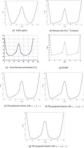
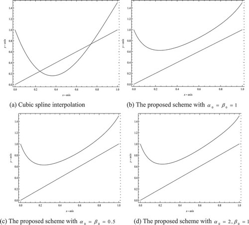
Example 4. Table 5 demonstrates the data lies above a straight line$y=x+2$ from Hussain and Hussain (2006). Figure 5(a) shows the cubic Hermite spline interpolation. Clearly cubic Hermite is unable to produce interpolating curve lie above straight line. Figure 5(b) shows the constrained data interpolation by using the method of Hussain and Hussain (2006). Figure 5(c) shows that the scheme of Sarfraz et al. (2005) fails to produce the interpolating curve with shape preservation. Figure 5(d) shows the interpolating curve by using Karim and Kong (2014) scheme. Figure 5(e) –5(g) shows the constrained data interpolation using the proposed scheme with ${\alpha }_i={\beta }_i=1$, ${\alpha }_i=1,{\beta }_i=2$ and ${\alpha }_i=1,{\beta }_i=4$ for all $i=0,1,\dots ,6$. The parameter ${\gamma }_i$ is calculated from Condition (29) and are given as ${\gamma }_i=\left\{0.1,0.1,1.785,14.05,0.1,0.1\right\}$ for Figure 5(e), ${\gamma }_i=\left\{0.1,0.1,1.785,4.05,0.1,0.1\right\}$ for Figure 5(f) and ${\gamma }_i=\left\{0.1,0.1,1.785,20.378,0.1,0.1\right\}$ for Figure 5(g), respectively. Figure 5(g) indicates that the bigger the value of ${\beta }_i$ will give loose curve and very visually pleasing. Compared to Karim and Kong (2014), the proposed scheme gives more visually pleasing results as well as the interpolating curve is very close to the constraint line while at the same time maintaining shape preservation. Therefore, by having two free parameters, ${\alpha }_i,{\beta }_i$, the interpolating curves can be changed interactively.

Table 5. A data set from Hussain and Hussain (2006)

$i$	0	1	2	3	4	5	6
$x_i$	0	2	4	10	28	30	32
$f_i$	22.8	12.8	10.2	12.5	33.9	38.9	43.6
$d_i$	−6.85	−3.15	−0.8792	0.5847	2.369	2.425	2.275

Figure 5. Interpolating curves generated by the proposed scheme and other existing schemes.

Example 5. Data in Table 6 lie above $y=0.5x+0.75$ .

Table 6. A data above straight line

$x_i$	0	0.4	1.5	2.2	2.5	3.9	5
$f_i$	2	1.2	1.8	3	4	5.8	5
$d_i$	−2.68	−1.32	1.26	2.85	2.97	0.58	−1.61

Figure 6(a) shows that the cubic spline interpolation cannot produce the interpolating curve lie above a straight line. Figure 6(b) until 6(d) shows the constrained data interpolation with the proposed scheme by using Theorem 2. The proposed scheme with ${\alpha }_i={\beta }_i=0.5$ give more visually pleasing result compare with the other interpolating curves.

Figure 6. Interpolating curves for data in Table 6.

Example 6. The data in Table 7 lie above two straight lines $y=x$.

Table 7. A data above straight line

$x_i$	0.0	1.0
$f_i$	1.0	1.5
$d_i$	−5.00	3.00

Figure 7(a) shows that the cubic spline interpolation with ${\alpha }_i={\beta }_i={\gamma }_i=1$ is not shape preserving interpolation to the constraint line. Figure 7(b) until 7(d) shows that the interpolating curve lies above the given constraint line by applying Theorem 2.

Figure 7. Various interpolating curves.

From all numerical and graphical results, we can conclude that, the proposed scheme is on par with some existing schemes. Furthermore, for some data sets, we show that various existing schemes are not shape preserving. For instance, for positive data in Table 2, the schemes proposed by Hussain et al. (2011) and Hussain et al. (2008) fail to preserve the positivity on the sub-interval (Hussain et al., 2011, 28). Sarfraz et al.’s (2005) scheme also fails to produce the interpolating curve lie above a constraint line. Furthermore, for data set in Table 6, the proposed scheme gives more visually pleasing result compared with the scheme of Karim and Kong (2014) and PCHIP. With all this examples and justification, the proposed scheme is suitable for positivity preserving and constrained data interpolation since the two free parameters ${\alpha }_i,{\beta }_i$, can be utilized to produce visually pleasing results while at the same time achieve the shape preservations.

5. Conclusion and future recommendation

To overcome the drawback in some shape preserving schemes, in this study a new type of rational cubic spline (cubic numerator and quadratic denominator) is constructed. It has three parameters ${\alpha }_i,{\beta }_i$, and ${\gamma }_i$, for all $i=0,1,\dots ,n-1$. This new rational spline (cubic/quadratic) is used for positivity preserving and constrained interpolation for data lie above arbitrary straight line. To achieve the shape preserving, we derive an automatic choice on one parameter ${\gamma }_i$, for $i=0,1,\dots ,n-1$ meanwhile the other two parameters ${\alpha }_i$ and ${\beta }_i$ can be used to modify the shape of the interpolating curve. Theorems 1 and 2 are guaranteed sufficient to produce the positive interpolating curve and constrained interpolating curve lie above arbitrary straight line. Work on monotonicity and convexity shape preserving interpolation by using the proposed scheme is underway including surface interpolation

Acknowledgement

This research is fully supported by Universiti Teknologi PETRONAS (UTP) through a research grant YUTP: 0153AA-H24 (Spline Triangulation for Spatial Interpolation of Geophysical Data).

Data Availability Statement

All data used in this study are obtained from other sources that have been cited in this paper.

Additional information

Funding

This work was supported by Universiti Teknologi PETRONAS (UTP), Spline Triangulation for Spatial Interpolation of Geophysical Data [grant number YUTP 0153AA-H24].

Notes on contributors

Samsul Ariffin Abdul Karim

Samsul Ariffin Abdul Karim is a senior lecturer at Fundamental and Applied Sciences Department, Universiti Teknologi PETRONAS (UTP). He has been in the department for more than 10 years. He obtained his BAppSc., MSc and PhD in Computational Mathematics & Computer Aided Geometric Design (CAGD) from Universiti Sains Malaysia (USM). He had 15 years of experience using Mathematica and MATLAB software for teaching and research activities. His research interests include curves and surfaces designing, geometric modelling and wavelets applications in image compression and statistics. He has published more than 110 papers in Journal and Conferences as well as seven books including two research monographs as well as one edited conference volumeand 10 book chapters. He was the recipient of Effective Education Delivery Award and Publication Award (Journal & Conference Paper), UTP Quality Day 2010, 2011 and 2012, respectively. He is Certified WOLFRAM Technology Associate, Mathematica Student Level.

References

- Abbas, M. , Majid, A. A. , M.N.Hj, A. , & Ali, J. M. (2012). Constrained shape preserving rational bi-cubic spline interpolation. World Applied Sciences Journal , 20(6), 790–800.
- Bashir, U. , & Ali, J. M. (2013). Data visualization using rational trigonometric spline. Journal of Applied Mathematics , 2013(Article ID 531497), 10. doi:10.1155/2013/531497
- Brodlie, K. W. , Asim, M. R. , & Unsworth, K. (2005). Constrained visualization using Shepard interpolation family. Computers and Graphics Forum , 24(4), 809–820. doi:10.1111/j.1467-8659.2005.00903.x
- Butt, S. , & Brodlie, K. W. (1993). Preserving positivity using piecewise cubic interpolation. Computer and Graphics , 17(1), 55–64. doi:10.1016/0097-8493(93)90051-A
- Fritsch, F. N. , & Carlson, R. E. (1980). Monotone piecewise cubic interpolation. SIAM Journal Numerical Analysis , 17, 238–246. doi:10.1137/0717021
- Hussain, M. Z. , & Ali, J. M. (2006). Positivity preserving piecewise rational cubic interpolation. Matematika , 22(2), 147–153.
- Hussain, M. Z. , & Hussain, M. (2006). Visualization of data subject to positive constraint. Journal of Information and Computing Sciences , 1(3), 149–160.
- Hussain, M. Z. , Hussain, M. , & Samreen, S. (2008). Visualization of shaped data by rational quartic spline interpolation. International Journal of Applied Mathematics & Statistics , 13(J08), 34–46.
- Hussain, M. Z. , Hussain, M. , & Waseem, A. (2014). Shape-preserving trigonometric functions. Computational and Applied Mathematics , 33, 411–431. doi:10.1007/s40314-013-0071-1
- Hussain, M. Z. , & Sarfraz, M. (2008). Positivity-Preserving interpolation of positive data by rational cubics. Journal of Computational and Applied Mathematics , 218, 446–458. doi:10.1016/j.cam.2007.05.023
- Hussain, M. Z. , Sarfraz, M. , & Shaikh, T. S. (2011). Shape preserving rational cubic spline for positive and convex data. Egyptian Informatics Journal , 12, 231–236. doi:10.1016/j.eij.2011.10.002
- Ibraheem, F. , Hussain, M. , Hussain, M. Z. , & Bhatti, A. A. (2012). Positive data visualization using trigonometric polynomials. Journal of Applied Mathematics , Article ID, 247120.
- Karim, S. A. A. (2013). Rational cubic ball functions for positivity preserving. Far East Journal of Mathematical Sciences (FJMS) , 82(2), 193–207.
- Karim, S. A. A. (2015a). Positivity preserving by using rational cubic ball function. AIP Conference Proceedings , 1660, 050049.
- Karim, S. A. A. (2015b). Shape preserving by using rational cubic ball interpolant. Far East Journal of Mathematical Sciences (FJMS) , 96(2), 211–230. doi:10.17654/FJMSJan2015_211_230
- Karim, S. A. A. (2016a). Data Interpolation using rational cubic Ball spline with three parameters. AIP Conference Proceedings , 1787, 080023.
- Karim, S. A. A. (2016b). Positivity preserving interpolation by using rational cubic ball spline. Jurnal Teknologi , 78(11), 141–148.
- Karim, S. A. A. , & Kong, V. P. (2014). (2014). Shape preserving interpolation using rational cubic spline. Research Journal of Applied Sciences, Engineering and Technology (RJASET) , 8(2), 167–168. doi:10.19026/rjaset.8.956
- Liu, S. , Che, Z. , & Zhu, Y. (2015). Rational quadratic trigonometric interpolation spline for data visualization. Mathematical Problems in Engineering , 2015(Article ID 983120), 20.
- Sarfraz, M. (2002). Visualization of Positive and Convex Data by a Rational Cubic Spline Interpolation , Information Sciences , 146(1–4), 239–254.
- Sarfraz, M. , Hussain, M. Z. , & Chaudary, F. S. (2005). Shape preserving cubic spline for data visualization. Computer Graphics and CAD/CAM , 01, 185–193.
- Sarfraz, M. , Hussain, M. Z. , & Nisar., A. (2010). Positive data modeling using spline function. Applied Mathematics and Computation , 216, 2036–2049. doi:10.1016/j.amc.2010.03.034
- Schmidt, J. W. , & Hess, W. (1988). Positivity of cubic polynomials on intervals and positive spline interpolation. BIT , 28, 340–352. doi:10.1007/BF01934097
- Wu, J. , Zhang, X. , & Peng, L. (2010). Positive approximation and interpolation using compactly supported radial basis functions. Mathematical Problems in Engineering , Article ID 964528, 10.