An Artificial neural networks (ANN) model for evaluating construction project performance based on coordination factors

Abstract

Construction projects are delivered in a multidisciplinary environment, which need continues coordination. The aim of this paper is to develop an ANN model to evaluate the influence of coordination factors on construction projects performance. For this purpose, the most effective 16 coordination factors impacting the construction projects performance have been identified. After that, through a questionnaire survey, the extent of coordination factors application and the corresponding project’s performance were collected. Three multilayer feed-forward networks with Back-Propagation and Elman-Propagation algorithms were adopted to train, validate, and test the cost, time and quality, as performance evaluation indicators. Consequently, the training process continues unit it reaches the pre-defined error or up to 1000 epochs. The results of Mean Square Error (MSE) confirmed the accuracy of the networks with an average value of 0.0231. Furthermore, the determination coefficient (R²) for the three networks of cost, time, and quality were obtained to be 0.77, 0.76 and 0.75, respectively.

Keywords:

• artificial neural networks
• performance evaluation
• construction projects

PUBLIC INTEREST STATEMENT

The construction industry is one of the significant contributors to the economic growth of any country. In developed countries, it incorporates the Gross Domestic Product (GDP) growth of about 7–10%, whereas in developing countries the contribution is 3–6%. However, the construction industry is inhibited by a low performance that often unfolds as cost and time overrun and poor quality. This low performance is because of the multidisciplinary nature of the construction projects and the participation of many stakeholders such as owners, contractors, subcontractors, and consultants. Construction projects are delivered in a multidisciplinary environment, which need continues coordination. This study developed a consistent model for evaluating construction projects performance in term of cost, time, and quality based on coordination factors. Although various modelling techniques developed for performance evaluation that incorporate the influence of different factors, ANN are found to have better pattern recognition and learning capabilities to get a reliable evaluation.

1. Introduction

The construction industry is one of the significant contributors to the economic growth of any country. In developed countries, it incorporates the Gross Domestic Product (GDP) growth of about 7–10%, whereas in developing countries the contribution is 3–6% (Ortiz, Castells, & Sonnemann, 2009). However, the construction industry is inhibited by a low performance that often unfolds as cost and time overrun and poor quality. This low performance is because of the multidisciplinary nature of the construction projects and the participation of many stakeholders such as owners, contractors, subcontractors, and consultants (Chan & Chan, 2004; Ward & Chapman, 2008). Recent research has shown that challenges due to the dependencies between the stakeholders are recurring problems in construction projects, particularly when the task involves more than one stakeholder. Therefore, the opportunity to improve projects performance through more efficient project management approaches like coordination could provide substantial enhancement. However, there is no existing tool to quantify the effect of coordination factors on construction projects performance (Alaloul, Liew, & Zawawi, 2016a; Beach, Webster, & Campbell, 2005; Yang & Shen, 2014).

The aim of this study is to develop a consistent model for evaluating construction projects performance in term of cost, time, and quality based on coordination factors. Although various modelling techniques developed for performance evaluation that incorporate the influence of different factors, ANN are found to have better pattern recognition and learning capabilities to get a reliable evaluation (Attalla & Hegazy, 2003). The most important 16 coordination factors were identified through Delph technique. Then, the extent of coordination factors application has been obtained through a questionnaire survey. Mostly, the relationships between the input (coordination factors) and outputs (project performance) were determined and tested. Several iterations of ANN architectures and algorithms were checked. Therefore, the connections between neurons (weights) were modified and retested until the best networks that fit the data were developed.

The construction industry carries out complex projects by separating them into smaller dependent sub-packages and allocated to different stakeholders (Yang & Shen, 2014). Thus, coordination ascends as a reply to those interdependent with sub-packages. However, several types of projects, in specific, non-routine knowledge intensive tasks as construction projects, are full of interdependencies which may adjust every day or hour and impact the performance adversely (Alaloul et al., 2016b). Based on the literature review, the majority of the previous research have applied regression models. These produced weak correlation due to incomplete information which reduced the model efficiency (Attalla & Hegazy, 2003; Tu, 1996). Ling and Liu (2004) stated that ANN models are robust if it is compared with conventional regression regarding projecting capability and pattern recognition. Dvir, Ben-David, Sadeh, and Shenhar (2006) also summarized that ANN models have stronger prediction power, and they support the developing of better associations between variables compared to any classical statistical approach. Therefore, the endeavours to apply linear or nonlinear regression for the projects performance evaluation should be upgraded to get a better representation of the relationships (Tu, 1996). ANN is the proposed alternative as a modelling tool to simulate the relationships between variables. In construction management, its application goes back to the early 1980s, which include extensive subjects like; budget estimation, decision-making, mark-up forecasting and production rate (Moselhi, Hegazy, & Fazio, 1991). Yitmen and Soujeri (2010) developed an ANN model to present the impact of change orders on construction project performance and disputes occurrence. For this purpose, various factors that describe the adverse effects of change orders on project performance from previous research have been used. Based on survey data, the model has been developed. Back-propagation of error was used as the learning algorithm. A total of 100,000 epochs at a learning rate of 0.6 and gradient descent with momentum algorithm were used to train the network. A momentum factor of 0.9 was selected to avoid oscillation in weight values. Finally, the best model was achieved in the 1000 epoch with 0.004 of Mean Square Error (MSE).

Heravi and Eslamdoost (2015) developed an ANN model for measuring and predicting labour productivity using multilayer feed-forward algorithm. The model was trained with a back-propagation algorithm with Bayesian regularization. The network was started with single hidden layer after that was increased to two hidden layers. Sigmoid was adapted for the hidden layers activation function. However, a linear function was used in the output layer. In the final model, the fit is reasonably significant for all data sets, as the MSE was 0.0234 with the R² value of 0.949.

Jha and Chockalingam (2009) used questionnaire survey data to develop a model for quality performance prediction via ANN. The model inputs designed to be 20 critical quality factors (eleven successes and nine failures). The best prediction model was found to be with one hidden layer content of five neurons and the network structure was feed-forward with back-propagation as learning algorithm which led to satisfied MSE of 0.044.

Based on the above review, most of the studies have dealt with cost, time and quality individually for performance evaluation, and none of them evaluated performance based on coordination factors. It can be concluded that a universal consensus among the investigators about the efficiency of ANN in modelling exists, especially for performance estimation and evaluation. This paper particularly considers quantification of the coordination factors effect on projects performance. This study builds upon the work of Alaloul, Liew, and Zawawi (2016), who explored 53 coordination factors from different disciplines. Through interviews and Delphi technique, the most important 16 coordination factors affecting construction projects performance were selected as the inputs for the proposed model in the current study. On the other hand, cost, time and quality (iron triangle) were selected as the model outputs.

2. Methodology

Initially, the identification of critical coordination factors affecting projects performance was carried out in the previous study by Wesam Salah Alaloul et al. (2016a). Based on systematic literature review 53 coordination factors were identified. A through interviews and the Delph technique were conducted to rank the coordination factors. The ranking criteria was based on the relative important index (RII). The key 16 factors were classified into five main groups based on the previous studies. Table 1 illustrates the identified factors, their groups, and the descriptions.

Table 1. The key coordination factors along with their groups

Group	Factor	Description	Sources
Planning and Scheduling (PSF)	X1: Plans (PLA)	Use or write briefing of project execution approaches, such plans cover those delivered by the owner/contractor/consultant	(Iyer & Jha, 2006)
	X2: Scheduling (SCH)	Prepare and update schedules to convey time-related information, based on the new and actual events	(Saram & Ahmed, 2001)
	X3: Meetings (MEE)	To exchange ideas, deal with conflicts and facilitate work, such as regular/irregular meetings	(Hossain, 2009)
	X4: All parties’ participation in plans (APP)	Liaison and communication with specialist consultants and nominated subcontractors to be involved in plan	(Chang & Shen, 2009)
Resource Management and Contacts (RMCF)	X5: Joint site visits (JSV)	To inspect a project’s performance by gathering, sharing, or confirming information on-site	(Iyer & Jha, 2006)
	X6: Team spirit (TEM)	Developing and receiving constructive inputs from all participants with an open mind	(Iyer & Jha, 2003)
	X7: Communication channels (COC)	Open wide and fast communication channels amongst all parties, structured or unstructured	(Hossain, 2009)
Records and Documentation (RDF)	X8: Record maintenance (REM)	All drawings, information, directives, verbal instructions, and documents received from each party to others, hard/soft copies	(Jaffar, Tharim, & Shuib, 2011)
	X9: Drawing documentation (DRD)	For overlapping activities’ coordination and giving execution plan of responsibilities to all parties involved	(Love, Irani, & Edwards, 2004)
Contract Implementation (CIF)	X10: Contract documents (COD)	Understanding generally, including contract articles, drawings, and specifications as complementary documents	(Iyer & Jha, 2003)
	X11: Maintaining contracts (MAC)	Documents and amendments to contracts, and obtaining specifications, and technical details	(Iyer & Jha, 2006)
	X12: Cleared payments (CLP)	The payment is appropriate with contract specified limits and consistent with the work progress status	(Simatupang, Wright, & Sridharan, 2002)
Quality and Value Engineering (QVF)	X13: Work integration (WOI)	From different subsystems and subcontractors to agree on detailed construction methods’ and specifications	(Saram & Ahmed, 2001)
	X14: Design and specification clarity (DSC)	To assign adequate time and resources for project implementation	(Iyer & Jha, 2006)
	X15: Quality assurance plan (QUA)	Prepare for the project quality in line with contract specification	(Iyer & Jha, 2003)
	X16: Value engineering (VAE)	Find new alternatives for higher specifications with less cost	(Chang & Shen, 2009)

After the coordination factors identification, the procedure to achieve the current study objectives is presented as a flowchart in Figure 1. The flowchart illustrates the main five stages adopted in the current research as: (1) collecting the necessary data; (2) preparing the data; (3) ANN architecture design; (4) train the network; and (5) post-training analysis and implementing the network. Each stage is discussed in details in the following paragraphs:

Figure 1. The methodology main five stages.

2.1. Data collection

The necessary data for this study was obtained by a closed-ended questionnaire that was distributed among the representative sample of the population. The population includes owners, consultant and contractors from the construction industry. The developed questionnaire was distributed after modifications based on the pilot study. Considering Cochran formula for calculating the sample size for large populations, based on 90% confidence level and 10% margin of error, the needed sample size (SS) is 322, as estimated from Equation (1) (Barlett, Kotrlik, & Higgins, 2001).

(1) $SS=\frac{Z^{2}P\left(1-P\right)}{c^2}$(1)

where: Z = Z value (e.g. 1.96 for 95% confidence level), p = percentage picking a choice, expressed as decimal (0.3 used for sample size needed) and c = confidence interval, expressed as decimal (e.g. .05 = ± 5).

In this study, a total of 610 questionnaires were sent out; however, 325 valid responses were received with 53.3% return rate of. During the questionnaire filling in, the respondents were asked to focus on one construction project to determine the extent of coordination factors application. The extent of the application was measured using 5-point Likert scale, as shown in Appendix A. Therefore, the input data was in ordinal format. In the last part of the questionnaire, the respondents estimated the project performance based on the variance percentage between the original project cost, time and quality and the actual status of the project performance.

To measure the internal consistency or reliability of the questionnaire Cronbach’s alpha method was applied. The reliability testing focuses on the consistency within a measuring instrument; which confirms that the questionnaires is generalizable and will produce similar results with similar populations (Gliem & Gliem, 2003). In this study, the value of alpha obtained was 0.78, which is higher than the acceptable threshold (0.70).

2.2. Data pre-processing

The model development effectiveness depends on the available data and its preparation. After data collection, three pre-processing procedures were conducted to increase the training process efficiency. These procedures are: (1) missing data, (2) outliers data and (3) normalize data (Wu, Chau, & Li, 2009).

In this study, the missing data problem was solved through average calculation. Out of the 325 data set entered, only seven values were missed and solved. At the same time, it is important to identify the outliers, which are observations with a unique combination of characteristics identifiable distinctly from most of the observations. There was no such similar encountered, as the questionnaire was designed with closed end questions from limited options in the inputs (i.e. Likert scale) and outputs as well. On the other hand, the normalization procedure is an important step, since mixing variables with large magnitudes and small magnitudes from the inputs and the outputs will confuse the learning algorithm on the effect of each variable. Accordingly, numeric inputs should be normalized to fall within a particular range like (−1 to 1). Such procedures should improve the density of the data over the problem domain and allow the network to converge faster and generalize better outputs (Rani, Kumar, & Togati, 2013).

2.3. ANN architecture design

The ANN approach is an information processing technique based on simulating the human brain. It is usually applied to establish forecast and evaluation models. ANN is defined as “a computational mechanism able to acquire, represent, and figure mapping from one multivariate space of information to another, given a set of data representing that mapping” (Rafiq, Bugmann, & Easterbrook, 2001). ANN is composed of many mutually connected neurons (interconnecting processing elements) grouped in layers. Usually, ANN has three types of layers i.e. input, hidden and output layers. The input layer receives data about the inquiry from outside. Hidden layer(s) does not connect to the outside but connects to other layers. The output layer sends the result outside. Networks types are classified according to the number of layers (one layered and multi-layered networks), connection type between neurons (layered, fully connected and cellular), and learning process (feed-forward and feedback) (Adeli & Wu, 1998). A typical architecture of the feed-forward ANN structure is shown in Figure 2.

Figure 2. Typical structure of feed-forward ANN.

In the feed-forward ANN, every input neuron has its weight coefficient. By multiplying those weight coefficients with the input signals and by summing that, the input signal from each neuron is calculated. In Figure 3, the input data are marked as X₁, X₂ and X₃ , and the weight coefficients are W₁, W₂ and W₃ , as a typical processing element. The connection between the signal’s source and neurons is determined by the weight coefficients. Positive weight coefficient means speeding synapse, and negative coefficient means inhibiting synapse. If W_ij = 0, it means that there is no connection between these two neurons. Neuron records the summed input impulse, which is equal to the sum of all input impulses: IJ = W₁X₁ + W₂X₂ + W₃X₃ , in addition to the Bias (θ_j ) which is another neuron parameter. The received impulse is processed through an appropriate activation function, f(IJ), and the output signal from the neuron is: y_i = f(IJ) = f (θ_j + ∑ w_ji x_i) (Attalla & Hegazy, 2003; Moselhi et al., 1991).

Figure 3. Processing element of ANN.

The primary purpose of the activation function is to determine whether the result from the summary impulse can generate an output or not. This function is associated with the neurons from the hidden layers. Usually, a continuous, nonlinear, and differentiable logistic function is used as an activation function. A common practice is to use the sigmoid function and tan-hyperbolic function as shown in Equations (2) and (3), respectively (Jha & Chockalingam, 2009). Where: I is the normalized value of the result of the summary function:

(2) $f\left(I\right)=\frac{1}{\left(1+e^{-I}\right)}$(2)

(3) $f\left(I\right)=\frac{e^I-e^{-I}}{e^I+e^{-I}}$(3)

Among the fitting algorithms approaches, Back-propagation and Elman-propagation algorithms based on a gradient descent optimization technique, are efficient approaches for training multiple layer networks. Gradient descent is the technique where parameters such as weight and biases are moved in the opposite direction to the error gradient. Therefore, each step down the gradient results in smaller errors until a minor error is achieved (Adeli & Mingyang, 1998; Yitmen & Soujeri, 2010).

The network architecture refers to the number of hidden layers and the number of hidden neurones. There is a direct relationship between the number of inputs and the network architecture. The best method is to start with one hidden layer and then increase to two hidden layers if the performance with one layer is not satisfactory. Increasing the number of neurones in the hidden layer will enhance the power of the network, but requires more computation and is more likely to produce over-fitting (Rafiq et al., 2001; Rani et al., 2013). A suitable network is the one that is just large enough to provide an adequate model fit. The input values X₁ to X₁₆ were arranged in an input vector such that x∈^16 × 1 which represent the 16 inputs of coordination factors (as shown in Table 1). The inputs were fed into the hidden layer neurons after multiplying by an input weight matrix W_h. Besides, to complete the structure of ANN at this stage, a bias vector b_h was also fed into the hidden layer. The neurons at the hidden layer produce an output y₁ based on the value of IJ using the sigmoid or tan hyperbolic functions. Then the result y₁ was interred to the output layer, which included one neuron in each network for cost, time and quality outputs, as shown in Figure 4.

Figure 4. The conceptual networks design.

The ANN networks chosen in the present study is a multi-layered with neurones in all layers fully connected in the feed-forward approach (Figure 4). After started by one hidden layer, the performance was not satisfactory, then two hidden layers were chosen. The optimal number of neurones is decided during the training process by trial and error (Adeli & Mingyang, 1998).

To achieve an efficient training, three parameters should be well defined namely; training/testing tolerance, learning rate and momentum factor (Heravi & Eslamdoost, 2015; Yu & Liu, 2002). Tolerance is a value that specifies how accurate the network’s output must be to consider as correct during training and testing. The most meaningful tolerance is specified as a percentage of the output range, rather than the output value. For example, a tolerance of 0.1 means that the output value must be within 10% of the range of the output to be considered correct. Selecting a tolerance that is too loose (large) or too tight (small) can cause an adverse impact on the network abilities. Therefore, in this study, the tolerance was set to 0.025 (Rani et al., 2013). Learning rate is the factor that determines the size of the steps that the network takes in navigating through the weight to minimize the error. For this study purpose, the learning rate of 0.7 or 0.8 was adjusted (Ling et al., 2004). On the other hand, the remedy for the problem of balancing the learning rate is to apply a momentum factor, which is multiplied by the previous weight change so that while the learning rate is controlled the changes are still rapid. A momentum factor of 0.9 was selected in this study (Jha & Chockalingam, 2009; Rani et al., 2013).

2.4. Training the network

Network training is the process that uses learning to modify weights or connections strength. All trial networks experimented in this study were trained in a supervised mode by a Back-propagation and Elman-propagation learning algorithms (Adeli & Mingyang, 1998). The collected data was divided into three subsets; 70% of the data (227 samples) are allocated for the training set, 15% (49 samples) for the validation set, and 15% (49 samples) for the test set. The training data set was presented to the network as inputs, and the outputs were calculated. The differences between the calculated outputs and the target outputs are evaluated and then used to adjust the network’s weights to reduce the differences until the error converges to an acceptable level (Attalla & Hegazy, 2003; Rani et al., 2013). Hence, it develops the input to output mapping by minimizing the MSE that is expressed in Equation 4:

4 $MSE=\frac{{\sum }_{i=1}^n{\left(O_i-P_i\right)}^2}{n}$4

where n is the number of samples in the training phase, O _i is the target output related to the sample i (i = 1, 2, 3…n), and P_i is the predicted output from the network.

The network training and development flowchart is presented in Figure 5. In the first condition, the Training Error Assessment (TEA) was checked. If the network passed this condition then the Testing Error Assessment (EA) need to be checked; otherwise, the network architecture needs to be revised. In case the network satisfies the second condition then it can be used to evaluate a new project’s performance (Adeli & Mingyang, 1998; Moselhi et al., 1991).

Figure 5. The network training and development flowchart.

2.5. Network validation and testing

ANN is purely empirical models; therefore, validation phase is critical to successful training and operation. The purpose of the network validation is to ensure its ability to generalize within limits set by the validation data in a robust fashion, rather than simply memorized the input-output relationships that are contained in the training data. If such performance is adequate, the model is deemed valid (Zhang, Hu, Patuwo, & Indro, 1999). During the training process, there will be more than one point after which the error rate typically begins to ascend because the generalization stopped improving and the over-fitting began. Therefore, when the validation error increases for a specified number of epochs, the training was halted, and the parameters corresponding to the minimum of this validation error were returned and saved. Network testing is essentially the same as validating it, except that the network is shown some data it has never seen before during the development process, and no corrections are made (Adeli & Mingyang, 1998; Attalla & Hegazy, 2003; Love et al., 2004).

3. Results and discussion

The results reported in this paper provides insights into the pattern of coordination factors and construction projects performance among the stakeholders working on construction projects. Many trails with various networks architectures were performed during the training process in order to achieve the best-trained network. The networks with two hidden layers show a better performance in comparison with one hidden layers networks. However, three hidden layers networks were also tested but did not result in any substantial performance improvement. The different trials for the three proposed networks, which were considered for cost evaluation, are shown in Table 1.

For cost evaluation network six trials were conducted. In Trial 1, the type of ANN used was FFBP whereas the L.A considered was TGDM with a log-Sigmoid transfer function by setting 1000 epochs and having five neurons in each hidden layer, with 0.7 and 0.9 for L.R and M.F, respectively. In Trial 2, the learning algorithm was changed from TGDM to TGD, the hidden neurons were increased from 5 to 10 in each hidden layer, and the L.R was changed from 0.7 to 0.8 while keeping all the other parameters constant. For Trial 3, similarly, the number of hidden neurons were increased to 15 in each hidden layer with the same learning algorithm. The transfer function was changed to Tan-Sigmoid for the two hidden layers. In Trial 4 and Trial 5, the FFEP type of the network has been used with same iterations of hidden neurones, L.R, M.F, T.F and epochs as Trials 2 and 3. Furthermore, Trial 6 was similar to Trial 3 except the Learning algorithm, which becomes LM. The performance of the networks iterations presented in Table 1 was compared based on the MSE to select the optimum network (Rafiq et al., 2001). The six trails illustrated that the MSE values changed through the trails, where the lowest MSE value of 0.0239 was achieved in Trail 2. As shown in Figure 6, the best validation performance (MSE) of Trail 2 occurred at 998 iterations as marked by the vertical dash line. No significant overfitting occurred with this iteration. The characteristics of both the validation and test curves are similar. The remarks above indicate acceptable results for the network.

Figure 6. Performance plot of cost predication model.

For time and quality evaluation networks, same trial procedure was repeated until it reaches the desired performance level as shown in Tables 2 and 3, respectively.

Table 2. ANN trials for time evaluation network

No.	Type	L.A.	H.N	L.R	M.F	T.F	Epochs	MSE
Trial 1	FFBP	TGDM	5,5	0.7	0.9	LogSigmoid	1000	0.0562
Trial 2	FFBP	TGD	10,10	0.8	0.9	LogSigmoid	1000	0.0263
Trial 3	FFBP	TGDM	15,15	0.7	0.9	TanSigmoid	1000	0.0349
Trial 4	FFEP	TGDM	10,10	0.7	0.9	LogSigmoid	1000	0.1356
Trial 5	FFEP	TGD	15,15	0.7	0.8	TanSigmoid	1000	0.1274
Trial 6	FFBP	LM	10,10	0.7	0.9	LogSigmoid	1000	0.0458

L.A.: Learning Algorithm, H.N: Hidden Neurons, L.R.: Learning Rate, M.F.: Momentum Factor, T.F: Transfer Function, FFBP: Feed Forward Back-Propagation, FFEP: Feed Forward Elman-Propagation, TGDM: Tangent Gradient Descent with Momentum, TGD: Tangent Gradient Descent, LM: Levenberg Marquardt.

Table 3. ANN trials for quality evaluation network

No.	Type	L.A.	H.N	L.R	M.F	T.F	Epochs	MSE
Trial 1	FFBP	TGDM	5,5	0.7	0.9	LogSigmoid	1000	0.0725
Trial 2	FFBP	TGD	10,10	0.9	0.9	LogSigmoid	1000	0.0445
Trial 3	FFBP	TGD	15,15	0.7	0.9	TanSigmoid	1000	0.0533
Trial 4	FFEP	TGD	15,15	0.8	0.9	LogSigmoid	1000	0.0656
Trial 5	FFEP	TGDM	10,10	0.7	0.9	TanSigmoid	1000	0.0191
Trial 6	FFBP	LM	10,10	0.7	0.9	LogSigmoid	1000	0.0298

For the time evaluation network, Trial 2 shows the least MSE (up to certain extent similar to cost evaluation network). However, for the quality evaluation network, Trial 5 shows the least MSE. The performance plot for the time evaluation model is shown in Figure 7. The three curves represent the change in the MSE with epochs for training, validation and testing. However, the best model was reached at epoch number 996 as marked by the vertical dash line. It is obvious that the network achieved better results during the training stage compared to the testing stage because the desired outputs of the test data are always unknown to the network.

Figure 7. Performance plot of time predication model.

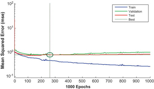
The performance plot for the quality evaluation network is shown in Figure 8. The three curves are representing the change in the MSE with epochs for training, validation and testing. However, the best model was reached in epoch number 281 as marked by the vertical dash line.

Figure 8. Performance plot of quality predication model.

To sum up, using the LogSigmoid function in the networks trained with TGDM brought less accurate results; however, the TGD exhibited a good response when used LogSigmoid. However, utilizing the TanSigmoid function with TGDM give better performance as in the quality evaluation network. It seemed that for both TGDM and TGD, choosing the same number of neurons for the hidden layers works well. Finally utilizing any function other than linear function in the output layer of the networks caused failing of the networks (Adeli & Mingyang, 1998; Heravi & Eslamdoost, 2015).

For models fitness and power assessment, the coefficient of determination (R²) was used, with 0.7 as a cut-off point (Taylor, 1990). From this study result, R² value for each network is larger than 0.7 as presented in Table 4. It can be concluded that the model has an exquisite explanatory power and suitable for evaluating the project performance. On the other hand, the most widely used test for detecting autocorrelation in the developed model is Durbin–Watson test that is denoted by “d” (Penda, Djellout, & Proïa, 2014). Its values when obtained from Equation (5) is often used to determine the accuracy and efficiency of prediction.

5 $d=2\left(1-\frac{\sum {\mu }_t-{\mu }_{t-1}}{\sum {\mu }_t^2}\right)$5

Table 4. Determination coefficient and Durbin–Watson test results

Network	R^2	Durbin–Watson
Cost evaluation network	0.77	1.65
Time evaluation network	0.765	1.78
Quality evaluation network	0.75	1.70

where ${\mu }_t$  = tp–op, tp and op are the observed and predicted values, respectively. The estimated “d” must lie within the range of (0 to 4). If there is no autocorrelation in the models, then, d value should be equal to two (d = 2), as a rule of thumb, that suggest the models are well estimated. The results of Durbin–Watson test for the current study yield a value very close to “2” as given in Table 4; therefore no auto-correlation was observed in the model (Penda et al., 2014).

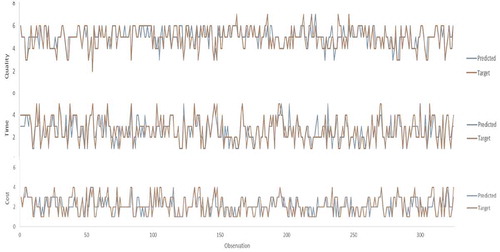
The concept of desired response and actual network output comparison is conducted as shown in Figure 9 after training process was completed for all data set of 325 samples. The gap between the two lines depicts the deviation between the two data sets for the three networks (cost, time and quality).

Figure 9. Predicted against target values for cost, time and quality networks.

Alternatively, residual plots need to be checked to grantee the model efficiency (Ling et al., 2004). The residual r_p, for pattern p, is simply the network output o_p minus the target t_p as shown in Equation (6):

(6) $\mathrm{r}\mathrm{p}=\mathrm{o}\mathrm{p}\text{-}\mathrm{t}\mathrm{p}$(6)

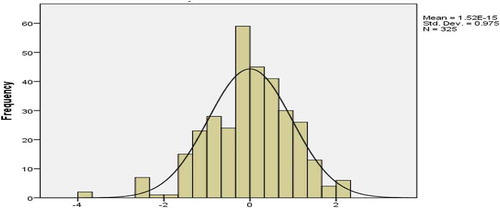
The histogram of the residual can be used to check whether the variance is normally distributed or not. A symmetric bell-shaped histogram, which is evenly distributed around zero, indicates that the normality assumption is likely to be true. If the histogram indicates that random error is not normally distributed, it suggests that the model’s underlying assumptions may have been violated (Ling et al., 2004; Rafiq et al., 2001). Figures 10, 11 and 12 illustrate an approximately normal distribution of residuals produced by cost, time and quality networks, respectively.

Figure 10. Histogram of residuals for cost network.

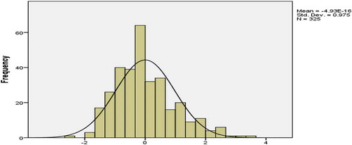
Figure 11. Histogram of residuals for time network.

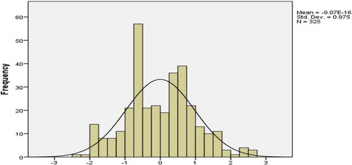
Figure 12. Histogram of residuals for quality network.

From the results of the extensive statistical tests, no technical problem with the model was observed, and it has qualified the tests prescribed for validation. Therefore, the model (including the three networks) was adapted effectively for evaluating construction projects performance.

4. Conclusions

Coordination factors are critical in construction projects success because of the multiple participants’ involvement during the project lifecycle. Therefore, the effects of coordination factors on project performance need to be investigated and quantified. This paper presents the relationship between coordination factors and construction project performance using ANN model owing to its robustness ability in pattern recognition and strong learning capability. A total of 325 data set, 16 coordination factors and the corresponding level of performance, were used to build the model. The model consists of three main networks to evaluate projects performance in term of cost, time and quality. Each network includes an input layer of 16 neurons corresponding to the 16 coordination factors, two hidden layers of 10 neurons and an output layer of a single neuron representing the performance indicator. Multilayer feed-forward neural networks with a Back-Propagation and Elman-Propagation algorithms were chosen. After many trials, the most appropriate network with the best generalization was selected. Based on the results, the proposed ANN model is efficient to evaluate the performance with respect to the mentioned coordination factors. Model accuracy was assessed by calculating the MSE which yielded 0.0239, 0.0263 and 0.0191 for cost, time and quality networks, respectively. The established model can be used as a decision-support tool by the project managers to evaluate the performance of construction projects through focusing on the key coordination factors to enhance the performance. In order to provide simple access to the developed model, a user interface may be developed to facilitate data input and to present the performance evaluation easily.

Acknowlegement

The authors would like to thank Universiti Teknologi PETRONAS Malaysia for financing the project under STIRF grant with code 0153AA-G37.

Additional information

Funding

The authors received no direct funding for this research.

Notes on contributors

Wesam Salah Alaloul

Wesam Salah Alaloul is currently a lecturer and researcher at Universiti Teknologi PETRONAS (UTP) Malaysia; He obtained his Ph.D. in 2016 at UTP Malaysia. His research interest is construction project management.

Mohd Shahir Liew

Mohd Shahir Liew currently a Professor at the Department of Civil Engineering, UTP Malaysia. He is also the Deputy Vice Chancellor Research and Innovation at UTP Malaysia.

Noor Amila Wan Zawawi

Noor Amila Wan Zawawi, PhD, is currently an Associate Professor at the Department of Civil and Environmental Engineering, UTP Malaysia. Her area of specialization includes Ocean Engineering, sustainable alternative use, Construction management and sustainability Building materials and technology.

Bashar S Mohammed

Bashar S Mohammed, PhD, is currently an Associate professor and Chair of the Department of Civil Engineering, UTP Malaysia. His research interest includes: rubberized concrete, rubberized interlocking bricks, reinforced concrete structures.

Musa Adamu

Musa Adamu completed his PhD in Civil Engineering at UTP Malaysia, and he is currently a lecturer in the department of civil Engineering, Bayero University Kano

References

- Adeli, H. , & Wu, M. (1998). Regularization neural network for construction cost estimation. Journal of Construction Engineering and Management , 124(1), 18–24.
- Alaloul, W. S. , Liew, M. S. , & Zawawi, N. A. B. W. A. (2016a). A framework for coordination process into construction projects . Paper presented at the MATEC Web of Conferences.
- Alaloul, W. S. , Liew, M. S. , & Zawawi, N. A. W. A. (2016b). Identification of coordination factors affecting building projects performance. Alexandria Engineering Journal , 55(3), 2689–2698.
- Attalla, M. , & Hegazy, T. (2003). Predicting cost deviation in reconstruction projects: Artificial neural networks versus regression. Journal of Construction Engineering and Management , 129(4), 405–411. doi:10.1061/(ASCE)0733-9364(2003)129:4(405)
- Barlett, J. E. , Kotrlik, J. W. , & Higgins, C. C. (2001). Organizational research: Determining appropriate sample size in survey research. Information Technology, Learning, and Performance Journal , 19(1), 43.
- Beach, R. , Webster, M. , & Campbell, K. M. (2005). An evaluation of partnership development in the construction industry. International Journal of Project Management , 23(8), 611–621. doi:10.1016/j.ijproman.2005.04.001
- Chan, A. P. C. , & Chan, A. P. L. (2004). Key performance indicators for measuring construction success. Benchmarking: an International Journal , 11(2), 203–221. doi:10.1108/14635770410532624
- Chang, A. S. , & Shen, F.-Y. (2009). Coordination needs and supply of construction projects. Engineering Management Journal , 21(4), 44–57. doi:10.1080/10429247.2009.11431844
- Dvir, D. , Ben-David, A. , Sadeh, A. , & Shenhar, A. J. (2006). Critical managerial factors affecting defense projects success: A comparison between neural network and regression analysis. Engineering Applications of Artificial Intelligence , 19(5), 535–543. doi:10.1016/j.engappai.2005.12.002
- Gliem, J. A. , & Gliem, R. R. (2003). Calculating, interpreting, and reporting Cronbach’s alpha reliability coefficient for Likert-type scales . Midwest research to practice conference in adult, continuing, and community education, Columbus, Ohio: Ohio State University.
- Heravi, G. , & Eslamdoost, E. (2015). Applying artificial neural networks for measuring and predicting construction-labor productivity. Journal of Construction Engineering and Management , 141(10), 04015032. doi:10.1061/(ASCE)CO.1943-7862.0001006
- Hossain, L. (2009). Communications and coordination in construction projects. Construction Management and Economics , 27(1), 25–39. doi:10.1080/01446190802558923
- Iyer, K. C. , & Jha, K. N. (2003). Analysis of critical coordination activities of Indian construction projects . Paper presented at the Proceedings of 19th annual conference of association of researchers in the construction management (ARCOM), University of Brighton, UK.
- Iyer, K. C. , & Jha, K. N. (2006). Critical factors affecting schedule performance: Evidence from Indian construction projects. Journal of Construction Engineering and Management , 132(8), 871–881. doi:10.1061/(ASCE)0733-9364(2006)132:8(871)
- Jaffar, N. , Tharim, A. H. A. , & Shuib, M. N. (2011). Factors of conflict in construction industry: A literature review. Procedia Engineering , 20, 193–202. doi:10.1016/j.proeng.2011.11.156
- Jha, K. N. , & Chockalingam, C. T. (2009). Prediction of quality performance using artificial neural networks: Evidence from Indian construction projects. Journal of Advances in Management Research , 6(1), 70–86. doi:10.1108/09727980910972172
- Ling, F. , Yng, Y. , & Liu, M. (2004). Using neural network to predict performance of design-build projects in Singapore. Building and Environment , 39(10), 1263–1274. doi:10.1016/j.buildenv.2004.02.008
- Love, P. E. D. , Irani, Z. , & Edwards, D. J. (2004). A rework reduction model for construction projects. IEEE Transactions on Engineering Management , 51(4), 426–440. doi:10.1109/TEM.2004.835092
- Moselhi, O. , Hegazy, T. , & Fazio, P. (1991). Neural networks as tools in construction. Journal of Construction Engineering and Management , 117(4), 606–625. doi:10.1061/(ASCE)0733-9364(1991)117:4(606)
- Ortiz, O. , Castells, F. , & Sonnemann, G. (2009). Sustainability in the construction industry: A review of recent developments based on LCA. Construction and Building Materials , 23(1), 28–39. doi:10.1016/j.conbuildmat.2007.11.012
- Penda, S. V. B. , Djellout, H. , & Proïa, F. (2014). Moderate deviations for the Durbin–Watson statistic related to the first-order autoregressive process. ESAIM: Probability and Statistics , 18, 308–331. doi:10.1051/ps/2013038
- Rafiq, M. Y. , Bugmann, G. , & Easterbrook, D. J. (2001). Neural network design for engineering applications. Computers & Structures , 79(17), 1541–1552. doi:10.1016/S0045-7949(01)00039-6
- Rani, C. H. S. , Kumar, V. P. , & Togati, V. K. (2013). Artificial neural networks (ANNS) for prediction of engineering properties of soils. International Journal of Innovative Technology and Exploring Engineering , 3(1), 123–130.
- Saram, D. D. D. , & Ahmed, S. M. (2001). Construction coordination activities: What is important and what consumes time. Journal of Management in Engineering , 17(4), 202–213. doi:10.1061/(ASCE)0742-597X(2001)17:4(202)
- Simatupang, T. M. , Wright, A. C. , & Sridharan, R. (2002). The knowledge of coordination for supply chain integration. Business Process Management Journal , 8(3), 289–308. doi:10.1108/14637150210428989
- Taylor, R. (1990). Interpretation of the correlation coefficient: A basic review. Journal of Diagnostic Medical Sonography , 6(1), 35–39. doi:10.1177/875647939000600106
- Tu, J. V. (1996). Advantages and disadvantages of using artificial neural networks versus logistic regression for predicting medical outcomes. Journal of Clinical Epidemiology , 49(11), 1225–1231.
- Ward, S. , & Chapman, C. (2008). Stakeholders and uncertainty management in projects. Construction Management and Economics , 26(6), 563–577. doi:10.1080/01446190801998708
- Wu, C. L. , Chau, K. W. , & Li, Y. S. (2009). Predicting monthly streamflow using data‐driven models coupled with data‐preprocessing techniques. Water Resources Research , 45, 8.
- Yang, R. J. , & Shen, G. Q. P. (2014). Framework for stakeholder management in construction projects. Journal of Management in Engineering , 31(4), 04014064. doi:10.1061/(ASCE)ME.1943-5479.0000285
- Yitmen, I. , & Soujeri, E. (2010). An artificial neural network model for estimating the influence of change orders on project performance and dispute resolution. Safety , 9, 3.
- Yu, C.-C. , & Liu, B.-D. (2002). A backpropagation algorithm with adaptive learning rate and momentum coefficient . Paper presented at the Neural Networks, IJCNN’02. Proceedings of the International Joint Conference on Neural Networks, IEEE, Honolulu, HI, USA.
- Zhang, G. , Hu, M. Y. , Patuwo, B. E. , & Indro, D. C. (1999). Artificial neural networks in bankruptcy prediction: General framework and cross-validation analysis. European Journal of Operational Research , 116(1), 16–32. doi:10.1016/S0377-2217(98)00051-4