A vendor–buyer inventory model with imperfect production considering investment to reduce lead time variability

Abstract

This research develops an integrated single-vendor single-buyer inventory model considering imperfect production process and investment to reduce lead time variance. In the model, we consider a system where the buyer’s lead time is uncertain and follows a normal distribution. Inspection process is performed by the buyer to classify the defective items in each lot delivered from the vendor. The defective items that were found by the buyer will be returned to the vendor at the next delivery. The shortages are allowed and assumed to be fully backordered. The objective function of the model is to minimize the expected joint total cost of the system by simultaneously determining the optimal shipment lot size, optimal safety factor, optimal target variance reduction of lead time and optimal number of shipments. Further, a numerical example is provided to illustrate the application of the proposed model. Based on the results, we understand that by applying the investment policy to reduce lead time variance, the system may improve its service level at a lower cost. Thus, we conclude that the investment policy is proved to give better outcomes to the system.

Keywords:

• inventory model
• lot sizing
• supply chain system
• lead time variance
• imperfect production
• shortage
• full backorder

PUBLIC INTEREST STATEMENT

The proposed study is interesting for researchers or practitioners working in inventory system. The model can help decision makers to manage inventories across supply chain efficiently by deciding the optimum quantity order, safety factor, number of deliveries and lead time variance. The supply chain system considered in this paper involves single vendor and single buyer. The vendor produces lots of items and delivers them to buyer equally. The vendor’s production system is imperfect; hence, it produces some defective items. The buyer faces stochastic demand and manages inventory using continuous review policy. Investment model formulated with logarithmic function is proposed to reduce lead time variance. Two models are developed and solved using an iterative procedure. The results show that by allowing the vendor to invest amount of money to reduce lead time variance, some benefits can be realized, including the reduction of joint total cost.

1. Introduction

As an integral part of the most businesses and industries, supply chain management has been broadly known as one essential key to company success. Companies should undergo a careful planning and design in order to perform an effective and successful supply chain to fulfil customer expectations at a manageable cost (Bala, 2014). Through an effective supply chain policies, companies can recognize significant benefits including reduced inventories and its related costs. Several inventory-related costs such as capital cost, investment to reduce setup costs, holding cost at the manufacturer, wholesaler and also the retailer can be significantly decreased by a good inventory management (Simchi-Levi, Kaminsky, & Simchi-Levi, 2008). This reality makes us aware that profits of all parties in the supply chain can be increased by improving the inventory management.

Hamontree, Ouelhadj and Beullens (2012) mentioned that inventory has a major contribution to the overall logistics costs. The individual decisions in reducing inventory costs do not lead to an optimal solution. Therefore, the coordination of central decisions along the supply chain is one method to obtain the best solution in inventory management. Since vendor–buyer system expects an increase in their mutual profit at a minimum total cost, they are trying to implement a strategy by coordinating and sharing information to achieve their common goals. Whereas in this case, the vendor acts as a manufacturer while the buyer is the one who buys the product from the vendor and distributes the product to the end customers.

The first researcher to discuss inventory management with supply chain coordination was Goyal (1976). He introduced a vendor–buyer inventory model with unlimited production rate and adopted a lot-for-lot policy to deliver products from the vendor to the buyer. Banarjee (1986) developed a limited vendor–buyer inventory model and takes the appropriate price-adjustment approach to minimize joint total cost between those parties. Furthermore, there are several developments in the related field of research with various considerations, including Goyal (1988), Hoque (2011) and Sajadieh and Larsen (2015).

The general assumption in the vendor–buyer-integrated inventory model is that all items are always produced in good quality. However, this assumption cannot be justified since the real condition of a production process is not perfect and produces an amount of items that are defective (deteriorate). Porteus (1986) was the first researcher to include imperfect production process in an economic order quantity model. Several researchers recommended a quality improvement policy to reduce the out of control probability of the production. Lee and Park (1991) developed an economic production quantity model considering the cost of rework and warranty for the defective items in a production process. Meanwhile, Jauhari (2014a) developed inventory models with imperfect production process and stochastic demand by taking into consideration variable lead time, shortage and investment efforts to reduce the out of control probability. Jauhari (2014b) also developed a vendor–buyer inventory model considering deterministic demand and defective rate that follow uniform distribution. Inventory models with imperfect production process were also developed by Lin (2010a), Lin (2010b), Sana (2010) and Dey and Giri (2014).

In the supply chain management, lead time is an important issue to measure the chain performance along with product quality and cost. Mostly in the field of supply chain inventory model, lead time is considered to be constant or deterministic, whereas in the real case, lead time is stochastic in nature. The existence of lead time in either production, setup, or delivery has one critical importance in both production and product distribution processes. The smaller the lead time variance in the supply chain, the better the process. When the variance of the lead time is high, it will increase the uncertainties of the system. Chaharsooghi and Heydari (2010) confirmed in their study that high variance in lead time is much more dangerous than the length (mean) of lead time.

One model considers that the lead time reduction is developed by Paknejad, Nasri and Affisco (1992). The study is inspired by how Japanese manufacturing companies reduce lead time uncertainty to establish good relationships with suppliers. They proposed an investment model to reduce the stochastic lead times. Hayya, Harrison and He (2011) classified lead time reduction into two components, i.e. reduction of mean lead time and reduction of lead time variance with exponential distribution. Meanwhile, Nasri, Paknejad and Affisco (2008) developed a single-echelon inventory model considering the existence of defective items and investment to reduce lead time. Lo (2013) developed inventory models considering an imperfect production process and reduction of lead time and setup costs. In the study, shortage during lead time is assumed to be partial backorder. Lin (2016) developed a vendor–buyer integrated inventory model to include shortage, stochastic lead time and investment effort to reduce lead time. In the model, Lin (2016) used exponential lead time and assumed that reducing the mean lead time will automatically reduce the lead time variance.

Investigations related to lead time reduction in the field of inventory modelling have been done by many researchers to focus only on mean lead time, whereas research in inventory model that examines the lead time variance reduction is still rare. Therefore, this research develops an inventory model with lead time variance reduction investment by adopting the basic model of Ganeshan, Kulkarni and Boone (2001) in which a quality improvement model was developed with a variance reduction investment to minimize Taguchi’s quality loss. The investment will reduce the value of current product variance to achieve variance reduction target. We adopt these concept developed by Ganeshan et al. (2001) and adjust it to the proposed model in which we examine a vendor–buyer inventory system with continuous review policy. We consider the existence of shortage and imperfect production process and include an investment to reduce the variance of normally distributed lead time.

The rest of this paper is organized as follows. The mathematical model development is described in Section 2. Section 3 presents the procedure to obtain optimal solution of the model. Section 4 discusses the sensitivity analysis of the model due to the several parameter uncertainties. Finally, Section 6 gives conclusion of the study.

2. Model development

2.1. System description

The material flow of the investigated vendor–buyer system is depicted in Figure 1. In the system, for each cycle of production process, the buyer orders a number of DT units to meet the end customer’s demand and the vendor produces a number of nDT at the rate of production, P. The annual production rate, P, is assumed to be fixed and greater than the demand (P > D). After the vendor is finished producing a number of DT units in the first batch, the vendor will deliver the products to the buyer and will be shipped n times per batch. In the system, the vendor will pay for the production setup cost, K, while the buyer bears the ordering cost, A, and the delivery cost, V.

Figure 1. The vendor–buyer system investigated in the model.

In the proposed inventory model, the production process performed by the vendor is not running perfectly. This will end up in a number of defective items received by the buyer. The buyer performs an inspection activity to classify whether the product is defective or not, with a cost of s $/unit and inspection rate of x unit/year. The portion of defective items, γ, is assumed to be deterministic. All products classified as defects will then be stored in the warehouse until the inspection process is completed. Those defective items will subsequently be returned to the vendor on the next shipment. Consequently, the buyer bears the cost to hold an amount of γDT units of defective items, with a holding cost of h _B $/unit/year. However, the buyer will eventually get a warranty refund from the vendor of w $/unit, by the existence of the defective products.

This model allows for shortages with full backorder policy. The buyer will incur a cost of π per unit backorder. In this case, the safety factor (k) is required as the standard deviation number of the mean corresponding to the desired service level. Safety factors are usually determined by the management. For example, k = 95% has the probability of 0.05 (α = 5%) that the number of orders at the time of lead time is higher than the safety stock. According to the standard normal distribution table Z, the value of α = 0.05 has the cumulative probability of Z = 1.65. The notation f _s(k) denotes the probability value of each occurrence of X, while F _s(k) is the cumulative distribution function expressing probability in the event interval of (−∞, x).

Here, we also consider an investment to reduce the lead time variance as adopted from Ganeshan et al. (2001). The current lead time variance (${\sigma }_0^2$) represents the variance during the production process, while the minimum lead time variance is the resulting variance based on the best capability of the production process. The investment aims to reduce the value of the current lead time variance (${\sigma }_0^2$) into the target variance (${\sigma }^2(I)$), where the reduction value depends on the amount of investment. The greater the amount of investment, the greater the variance reduction will be. The coefficient of lead time variance reduction, b, is the function coefficient of the magnitude of reduction in variance for a certain amount of investment. We use the fractional cost of variance reduction, θ, in the calculation of the investment cost, I.

2.2. Mathematical model formulation

This paper develops an integrated inventory model of a single-vendor single-buyer system considering an imperfect production and shortage as full backordering. We include an investment for lead time variance reduction in which the function of variance reduction to the amount of investment is adopted from Ganeshan et al. (2001). The objective of the proposed model is to minimize the annual joint total cost between the vendor and the buyer by determining several decision variables as follow:

q*: optimal shipment lot size (unit/shipment)

n*: number of shipments (/year)

k* : safety factor

${\sigma }^2(I)$: lead time variance reduction target

We assume that the demand is deterministic, while the lead time is normally distributed with mean = μ and variance = σ ². The following inventory-related costs are considered in the model:

1. Holding costs at both vendor (HC_V) and buyer (HC_B) inventories,

2. Delivery cost from the vendor to the buyer (DC_B),

3. Buyer ordering cost (OC_B),

4. Buyer inspection cost (IC_B),

5. Buyer backordering cost (BC_B),

6. Vendor production set-up cost (SC_V),

7. Vendor cost of production (PC_V),

8. Vendor warranty cost (WC_V),

9. Investment cost to reduce lead time variance (IC_V).

The parameters used in the proposed model are expressed by the following notations.

Table

D: annual demand rate (unit/year)	γ: defective item proportion
P: annual production rate (unit/year) K: production set-up cost ($/batch)	δ: upper limit of the probability function of defective products
A: buyer ordering cost ($/order)	w: warranty cost ($/unit)
V: vendor delivery cost ($/shipment)	f s(k): probability density function for k
h V: vendor annual holding cost per unit product ($/unit/year) h B: buyer annual holding cost per unit product ($/unit/year)	F s(k): cumulative density function for k π: backordering cost ($/unit) ${\sigma }_0^2$: current lead time variance (days) ${\sigma }_{\mathrm{L}}^2$: minimum lead time variance (days)
a 1: production fixed cost ($)	${\sigma }^2(\mathrm{I})$: target lead time variance (days)
a 2: production variable cost ($/unit)	I: the amount of investment ($)
x: buyer inspection rate (unit/year)	b: variance reduction coefficient
s: buyer inspection cost ($/unit)	θ: fractional opportunity cost ($)

Here are several assumptions used in the model:

1. Production rate is always greater than the demand rate (P > D).

2. Demand (D) is deterministic.

3. Lead time is normally distributed.

4. Lead time can be shortened to the target value of σ ²(I) through a certain amount of lead time investment.

5. The relationship between the lead time variance reduction (σ ²(I)) and the amount of investment (I) is known and follows the function of ${\sigma }^2\left(I\right)={\sigma }_{\mathrm{L}}^2+\left({\sigma }_0^2-{\sigma }_{\mathrm{L}}^2\right)exp\left(-\mathrm{b}\mathrm{I}\right)$ with b > 0 (Ganeshan et al., 2001).

6. In each lot delivered to the buyer, there is always a portion of defective items with a probability of γ that follows a normal distribution.

We develop two scenarios in this study. Scenario I is the scenario without investment, and Scenario II is the one with investment. The results from both scenarios are then compared one to another in order to find out which one gives better outcome to the system. Inventory profiles for the vendor and the buyer are depicted in Figure 2.

Figure 2. On-hand stock level at vendor and buyer inventory (n = 5).

2.3. Without investment

For Scenario I, the inventory cost related to the vendor (TCV _I) consists of holding cost (HC_V ), production cost (PC_V ), production set-up cost (SC_V ) and warranty cost (WC_V ). The annual vendor holding cost (HC_V ) can be calculated as

(1) $H{C}_V=h_v\frac{q}{2}\left(n\left(1-\frac{D}{P}\left(E\left(\frac{1}{1-\gamma }\right)\right)\right)+\frac{2D}{P}\left(E\left(\frac{1}{1-\gamma }\right)\right)-1\right)$(1)

Vendor production cost (PC_V ) includes fixed cost and variable cost of production. The function of PC_V is formulated as follows:

(2) $P{C}_V=D\left(\frac{a_1}{\mathrm{P}}+a_{2}P\right)\left(E\left(\frac{1}{1-\gamma }\right)\right)$(2)

Vendor setup cost (SC_V ) is incurred at the beginning of each cycle of production process. The function of SC_V is formulated as follows:

(3) $S{C}_V=\frac{DK}{nq}\left(E\left(\frac{1}{1-\gamma }\right)\right)$(3)

Vendor warranty cost (WC_V ) is given from the vendor to the buyer as a consequence of the defective products. The function of WC_V is given as follows:

(4) $W{C}_V=wD\left(E\left(\frac{1}{1-\gamma }\right)\right)$(4)

Thus, the function of TC_V for Scenario I is given as

(5) $TC{V}_I=H{C}_V+P{C}_V+S{\mathrm{C}}_V+W{C}_V$(5)

For the buyer side, the inventory cost for Scenario I includes holding cost (HC_B ), ordering cost (OC_B ), delivery cost (DC_B ), inspection cost (IC_B ) and cost of backorder (BC_B ). The annual buyer holding cost (HC_B ) for Scenario I can be calculated as

(6) $H{C}_B=h_b\left(\frac{qD}{x}\left(E\left(\frac{1}{1-\gamma }\right)\right)+\frac{q}{2}\left[1-E\left(\gamma \right)\right]+kD{\sigma }_0\right)$(6)

Buyer ordering cost (OC_B ) is incurred for each order made by the buyer to the vendor. The function of OC_B is formulated as follows:

(7) $O{C}_B=\frac{DA}{nq}\left(E\left(\frac{1}{1-\gamma }\right)\right)$(7)

Delivery cost (DC_B ) is the cost of transportation, incurred to the buyer, for every shipment made by the vendor. The function of DC_B is given by the equation below:

(8) $D{C}_B=\frac{DV}{q}\left(E\left(\frac{1}{1-\gamma }\right)\right)$(8)

Inspection cost (IC_B ) is the buyer cost to inspect each lot delivered by the vendor, since there may be defective items in it. The amount of IC_B is given below:

(9) $I{C}_B=sD\left(E\left(\frac{1}{1-\gamma }\right)\right)$(9)

The existence of lead time uncertainty in the system causes the possibility of the buyer to experience shortages. When there is a shortage of inventory, the buyer gives it as a backorder in which demand must be met in the next period with additional costs known as backordering cost. For Scenario I, the amount of buyer backordering cost (BC_B ) can be calculated as

(10) $B{C}_B=\frac{D^2}{nq}\pi {\sigma }_0\psi \left(k\right)\left(E\left(\frac{1}{1-\gamma }\right)\right)$(10)

with

(11) $\psi \left(k\right)=\left\{f_s\left(k\right)-k\left[1-F_{ms}\left(k\right)\right]\right\}$(11)

F _s(k) is the cumulative distribution function for k and f _s(k) is the probability density function for k following the standard normal distribution with μ = 0 and σ = 1.

Accordingly, the function of TCB _I for Scenario I is given as

(12) $TC{B}_{\mathrm{I}}=H{C}_B+O{C}_B+D{C}_B+I{C}_B+B{C}_B$(12)

For Scenario I, the expected joint total inventory cost (EJTC _I(q, n, k)) for the system is then formulated as

(13) $\begin{array}{rl}& EJT{C}_{\mathrm{I}}\left(q,n,k\right)=TC{V}_{\mathrm{I}}+TC{B}_{\mathrm{I}}\\ & =h_v\frac{q}{2}\left(n\left(1-\frac{D}{P}\left(E\left(\frac{1}{1-\gamma }\right)\right)\right)+\frac{2D}{P}\left(E\left(\frac{1}{1-\gamma }\right)\right)-1\right)\\ & +D\left(\frac{a_1}{P}+a_{2}P\right)\left(E\left(\frac{1}{1-\gamma }\right)\right)+\frac{DK}{nq}\left(E\left(\frac{1}{1-\gamma }\right)\right)+wD\left(E\left(\frac{1}{1-\gamma }\right)\right)\\ & +h_b\left(\frac{qD}{x}\left(E\left(\frac{1}{1-\gamma }\right)\right)+\frac{q}{2}\left[1-E\left(\gamma \right)\right]+kD{\sigma }_0\right)+\frac{DA}{nq}\left(E\left(\frac{1}{1-\gamma }\right)\right)\\ & +\frac{DV}{q}\left(E\left(\frac{1}{1-\gamma }\right)\right)+sD\left(E\left(\frac{1}{1-\gamma }\right)\right)+\frac{D^2}{nq}\pi {\sigma }_0\psi \left(k\right)\left(E\left(\frac{1}{1-\gamma }\right)\right)\end{array}$(13)

With Investment

In Scenario II, TCV _II consists of HC_V, PC_V, SC_V, WC_V and investment cost to reduce lead time variance (IC_V ). The functions of HC_V, PC_V, SC_V and WC_V have already been given by Equation (1), (2), (3) and (4), respectively, whereas the function of IC_V is formulated as follows:

(14) $I{C}_V=\alpha \frac{1}{b}ln\left(\frac{{\sigma }^2(I)-{\sigma }_L^2}{{\sigma }_0^2-{\sigma }_L^2}\right)$(14)

The above investment function is different from the formulations used by previous researchers (Paknejad et al., 1992; Nasri et al., 2008; Lin, 2016). The proposed formulation considers a minimum lead time variance as one of parameters needed to calculate the investment, while in the previous published papers, the researchers neglected a minimum lead time variance parameter and assumed that its value is always 0. In practice, however, reducing the lead time variance to be 0 would be too difficult since there are some unpredictable conditions in delivery process, production activity, material handling etc. So, here, we propose a model which gives an opportunity to decision makers to determine the minimum lead time variance based on their best process performance.

Therefore, the function of TCV _II becomes

(15) $TC{V}_{\mathrm{I}\mathrm{I}}=H{C}_V+P{C}_V+S{C}_V+W{C}_V+I{C}_V$(15)

Buyer total inventory cost for Scenario II (TCB _II) is similar to Scenario I except the formulation of HC_B and BC_B due to investment in the vendor. The function of HC_B and BC_B is calculated by Equations (16) and (17), respectively.

(16) $H{C}_B=h_b\left(\frac{qD}{x}\left(E\left(\frac{1}{1-\gamma }\right)\right)+\frac{q}{2}\left[1-E\left(\gamma \right)\right]+kD\sigma \left[I\right]\right)$(16)

(17) $B{C}_B=\frac{D^2}{nq}\pi \sigma \left[I\right]\psi \left(k\right)\left(E\left(\frac{1}{1-\gamma }\right)\right)$(17)

Finally, the expected joint total inventory cost (EJTC _II(q, n, k, ${\sigma }^2\left(I\right)$)) for Scenario II is formulated as

(18) $\begin{array}{rl}& EJT{C}_{\mathrm{I}\mathrm{I}}\left(q,n,k,{\sigma }^2\left(I\right)\right)=TC{V}_{\mathrm{I}\mathrm{I}}+TC{B}_{\mathrm{I}\mathrm{I}}\\ & =h_v\frac{q}{2}\left(n\left(1-\frac{D}{P}\left(E\left(\frac{1}{1-\gamma }\right)\right)\right)+\frac{2D}{P}\left(E\left(\frac{1}{1-\gamma }\right)\right)-1\right)\\ & +D\left(\frac{a_1}{P}+a_{2}P\right)\left(E\left(\frac{1}{1-\gamma }\right)\right)+\frac{DK}{nq}\left(E\left(\frac{1}{1-\gamma }\right)\right)+wD\left(E\left(\frac{1}{1-\gamma }\right)\right)\\ & -\alpha \frac{1}{b}ln\left(\frac{{\sigma }^2(I)-{\sigma }_L^2}{{\sigma }_0^2-{\sigma }_L^2}\right)+\frac{DA}{nq}\left(E\left(\frac{1}{1-\gamma }\right)\right)+\frac{DV}{q}\left(E\left(\frac{1}{1-\gamma }\right)\right)\\ & +h_b\left(\frac{qD}{x}\left(E\left(\frac{1}{1-\gamma }\right)\right)+\frac{q}{2}\left[1-E\left(\gamma \right)\right]+kD\sigma \left[I\right]\right)\\ & +sD\left(E\left(\frac{1}{1-\gamma }\right)\right)+\frac{D^2}{nq}\pi \sigma \left[I\right]\psi \left(k\right)\left(E\left(\frac{1}{1-\gamma }\right)\right)\end{array}$(18)

3. Solution procedure

The proposed models aim to minimize the expected joint total cost (EJTC) and determine the optimal value of q, k and σ ²(I). Beforehand, let us present the properties of the proposed models, in particular the expected joint total cost functions (EJTC) for both Scenario I and II.

Property 1: For fixed k, the function of EJTC_I(q, k) is convex in q

Proof: Taking the second partial derivation of EJTC _I(q, k) in Equation (13) w.r.t. q, we get

(19) $\frac{{\mathrm{\partial }}^{2}EJT{C}_{\mathrm{I}}}{\mathrm{\partial }{q}^2}=\frac{2D}{q^3}\left(E\left(\frac{1}{1-\gamma }\right)\right)\left(\frac{K}{n}+\frac{A}{n}+V+\frac{D}{n}\pi {\sigma }_0\psi \left(k\right)\right)>0$(19)

Property 2: For fixed k, the function of EJTC_II(q, k,$\sigma \left(I\right)$ ) is convex in q

Proof: Taking the second partial derivative of EJTC _II(q, k, $\sigma \left(I\right)$) in Equation (18) w.r.t. q, we get

(20) $\frac{{\mathrm{\partial }}^{2}EJT{C}_{\mathrm{I}\mathrm{I}}}{\mathrm{\partial }{q}^2}=\frac{2D}{q^3}\left(E\left(\frac{1}{1-\gamma }\right)\right)\left(\frac{K}{n}+\frac{A}{n}+V+\frac{D}{n}\pi \sigma \left(I\right)\psi \left(k\right)\right)>0$(20)

Property 3: For fixed q, the function of EJTC _I (q, k) is convex in k

Proof: Taking the second partial derivative of EJTC _I(q, k) in Equation (13) w.r.t. k, we get

(21) $\frac{{\mathrm{\partial }}^{2}EJT{C}_{\mathrm{I}}}{\mathrm{\partial }{q}^2}=\frac{D^2}{nq}\pi {\sigma }_0{f}_s\left(k\right)\left(E\left(\frac{1}{1-\gamma }\right)\right)>0$(21)

Property 4: For fixed q, the function of EJTC_II(q, k,$\sigma \left(I\right)$) is convex in k

Proof: Taking the second partial derivative of EJTC _II(q, k, $\sigma \left(I\right)$) in Equation (18) w.r.t. k, we get

(22) $\frac{{\mathrm{\partial }}^{2}EJT{C}_{\mathrm{I}\mathrm{I}}}{\mathrm{\partial }{q}^2}=\frac{D^2}{nq}\pi \sigma \left(I\right)f_s\left(k\right)\left(E\left(\frac{1}{1-\gamma }\right)\right)>0$(22)

The optimal value of q*, k* and σ*(I) for Scenario I and II can be found by setting the first partial derivation of EJTC w.r.t q, k and $\sigma \left(I\right)$, set the results equal to 0 and solve the equations, respectively. Accordingly, we obtain the formula of q*, k* and σ*(I) for Scenario I and II as follows:

Scenario I: Without Investment

(24) $q_I^{\ast }=\sqrt{\frac{E\left(\frac{1}{1-\gamma }\right)D\left(\frac{K}{n}+\frac{A}{n}+V+\frac{D}{n}\pi {\sigma }_0\psi (k)\right)}{\frac{h_v}{2}\left(n\left[1-E\left(\frac{1}{1-\gamma }\right)\frac{D}{P}\right]-1+E\left(\frac{1}{1-\gamma }\right)\frac{2D}{P}\right)+h_b\left(E\left(\frac{1}{1-\gamma }\right)\frac{D}{x}+\frac{\left[1-E(\gamma )\right]}{2}\right)}}$(24)

(25) $F_s{\left(k\right)}_{\mathrm{I}}^{\ast }=\left(1-\frac{h_{b}nq}{E\left(\frac{1}{1-\gamma }\right)D\pi }\right)$(25)

Scenario II: With Investment

(26) $q_{\mathrm{I}\mathrm{I}}^{\ast }=\sqrt{\frac{E\left(\frac{1}{1-\gamma }\right)D\left(\frac{K}{n}+\frac{A}{n}+V+\frac{D}{n}\pi \sigma \left(I\right)\psi (k)\right)}{\frac{h_v}{2}\left(n\left[1-E\left(\frac{1}{1-\gamma }\right)\frac{D}{P}\right]-1+E\left(\frac{1}{1-\gamma }\right)\frac{2D}{P}\right)+h_b\left(E\left(\frac{1}{1-\gamma }\right)\frac{D}{x}+\frac{\left[1-E(\gamma )\right]}{2}\right)}}$(26)

(27) $F_s{\left(k\right)}_{\mathrm{I}\mathrm{I}}^{\ast }=\left(1-\frac{h_{b}nq}{E\left(\frac{1}{1-\gamma }\right)D\pi }\right)$(27)

(28) ${\sigma }^2{\left(I\right)}_{\mathrm{I}\mathrm{I}}^{\ast }=\frac{2\alpha \sqrt{{\sigma }^2\left(I\right)}}{b\left(h_{b}kD+E\left(\frac{1}{1-\gamma }\right)\frac{D^2}{nq}\pi \psi (k)\right)}+{{\sigma }_L}^2$(28)

Here, we also develop a set of procedure, for both Scenario I and II, to find the optimal solution of the problems. The algorithm is presented below:

• Step 0. Set n = 1 and $EJT{C}_j\left(q_{n-1},k_{n-1},{\sigma }^2{\left(I\right)}_{n-1},n-1\right)=\mathrm{\infty }$

• Step 1. Start with shipment size

(29) $q_n=\sqrt{\frac{E\left(\frac{1}{1-\gamma }\right)D\left(\frac{K}{n}+\frac{A}{n}+V\right)}{\frac{h_v}{2}\left(n\left[1-E\left(\frac{1}{1-\gamma }\right)\frac{D}{P}\right]-1+E\left(\frac{1}{1-\gamma }\right)\frac{2D}{P}\right)+h_b\left(E\left(\frac{1}{1-\gamma }\right)\frac{D}{x}+\frac{\left[1-E(\gamma )\right]}{2}\right)}}$(29)

• Step 2. Start with ${\sigma }^2{(I)}_n={\sigma }_0^2$.

• Step 3. Substitute q_n from step 1 into $k_n$ (in Equation (25) for Scenario I, and in Equation (27) for Scenario II).

• Step 4. Using the value of $k_{\mathrm{n}}$ generated from Step 3, compute the value of ${\sigma }^2{\left(I\right)}_n$ in Equation (28) (only for Scenario II, skip this step for Scenario I).

• Step 5. Using the value of $k_n$ and ${\sigma }^2{\left(I\right)}_n$ obtained from Step 3 and 4, find the value of q_n (in Equation (24) for Scenario I, and in Equation (26) for Scenario II).

• Step 6. Repeat steps 1–5 until no change occurs in the values of q_n, k_n and ${\sigma }^2{\left(I\right)}_{\mathrm{n}}$.

• Step 7. Calculate EJTC(q_n, σ ²(I) _n, k_n, n) using Equation (13) for Scenario I and Equation (18) for Scenario II.

• Step 8. If EJTC(q_n, σ ²(I) _n, k_n, n) ≤ EJTC($q_{n-1}$, ${\sigma }^2{\left(I\right)}_{n-1}$, $k_{n-1}$, $n-1$), then repeat steps 1–7 with n = n + 1. Otherwise go to step 9.

• Step 9. Set EJTC(q*, σ ²(I)*, k*, n*) = EJTC($q_{n-1}$, ${\sigma }^2{\left(I\right)}_{n-1}$, $k_{n-1}$, $n-1$), and q* = $q_{n-1}$, σ ²(I)* = ${\sigma }^2{\left(I\right)}_{\mathrm{n}-1}$, k* = $k_{n-1}$ and n* = ($n-1$).

4. Numerical example

In this section, we provide a numerical example for each parameter to illustrate the application of the proposed model. The following data were taken from the previous studies (Ganeshan et al., 2001; Jauhari, 2018):

Table

D: 1,000 units/year	x: 7,000 unit/year	θ: $0.1/year
P: 3,000 units/year	п: $75/unit	σ^2 0: 0.01
A: $100/order	s: $0.5/unit	σ^2 L: 0.005
K: $400/setup	w: $2/unit	b: 0.0035
V: $50/delivery	a 1: $2,500/unit	δ: 0.04
h v: $6/unit/year	a 1: $0.0004/unit
h b: $10/unit/year

The probability density function for the defective items proportion is given as

(30) $\begin{array}{rl}& \\ & f(\gamma )=\left\{\begin{array}{cc}\frac{1}{\delta }& 0\le \gamma \le \delta \\ 0& \mathrm{o}\mathrm{t}\mathrm{h}\mathrm{e}\mathrm{r}\mathrm{w}\mathrm{i}\mathrm{s}\mathrm{e}\end{array}\right.=\left\{\begin{array}{cc}\frac{1}{(0.04)}& =250\le \mathrm{y}\le 0.04\\ 0& \mathrm{o}\mathrm{t}\mathrm{h}\mathrm{e}\mathrm{r}\mathrm{w}\mathrm{i}\mathrm{s}\mathrm{e}\end{array}\right.\\ & \\ & \end{array}$(30)

Hence, the expectation value for the defective items can be calculated as follows:

(31) $E\left(\gamma \right)=\underset{0}{\overset{0.04}{\int }}25\gamma d\gamma =0.02$(31)

(32) $E\left(\frac{1}{1-\gamma }\right)=\underset{0}{\overset{0.04}{\int }}\left(\frac{25}{1-\gamma }\right)d\gamma =1.0205$(32)

Applying the solution procedure presented in the previous section, we generate the optimization result for Scenario I and II as summarized in Table 1.

Table 1. The optimization result for the proposed model (1 ≤ ζ ≤ 10)

Scenario	n	q* (unit/lot)	k*	σ ^2(I)*	TCV (/year)	TCB (/year)	EJTC (/year)
Scenario I	1	344	1.69	–	$3,654.9	$1,714.8	$5,369.7
	2*	226*	1.56*	–	$3,697.9*	$1,665.8*	$5,363.7*
	3	174	1.49	–	$3,764.3	$1,680.3	$5,444.6
Scenario II	1	333	1.71	0.0052	$3,775.0	$1,561.0	$5,336.0
	2*	217*	1.58*	0.0052*	$3,799.3*	$1,515.5*	$5,314.7*
	3	167	1.51	0.0052	$3,852.9	$1,533.0	$5,385.9

Note: * optimal solutions

Based on Table 1, the optimal solutions for the given problem that minimize the expected joint total cost for Scenario I, when the vendor does not make any investment, are

• Optimal lot size ($q_{\mathrm{I}}^{\ast }$) = 226 units/lot

• Optimal number of shipments ($n_{\mathrm{I}}^{\ast }$) = 2 shipments/production cycle

• Optimal safety factor ($k_{\mathrm{I}}^{\ast }$) = 1.56

• Number of production cycle $\left(\frac{D}{nQ}\right)$ = $\frac{1000}{\left(2\times 226\right)}=2.21\approx 3\mathrm{c}\mathrm{y}\mathrm{c}\mathrm{l}\mathrm{e}\mathrm{s}/\mathrm{y}\mathrm{e}\mathrm{a}\mathrm{r}$

• Total number of shipments = 2× 3 = 6 shipments/year

For Scenario II, when the vendor makes an investment, the optimal solutions are

• Optimal lot size ($q_{\mathrm{I}\mathrm{I}}^{\ast }$) = 217 units/lot

• Optimal number of shipments ($n_{\mathrm{I}\mathrm{I}}^{\ast }$) = 2 shipments/production cycle

• Optimal safety factor ($k_{\mathrm{I}\mathrm{I}}^{\ast }$) = 1.58

• Optimal lead time variance reduction (σ ²(I)) = 0.0052

• Optimal amount of investment (I(σ ²)) = $903.62

• Number of production cycle $\left(\frac{D}{nQ}\right)$ = $\frac{1000}{\left(2\times 217\right)}=2.304\approx 3\mathrm{c}\mathrm{y}\mathrm{c}\mathrm{l}\mathrm{e}\mathrm{s}/\mathrm{y}\mathrm{e}\mathrm{a}\mathrm{r}$

• Total number of shipments = 2× 3 = 6 shipments/year

From the above comparison (see Table 1), we realize that Scenario II actually provides a set of solutions with less cost rather than Scenario I. In addition, the safety factor, k, of Scenario II is better than Scenario I. Therefore, decision to invest some money to reduce the lead time variance is proved to give better outcomes to the vendor–buyer system. The next section will discuss about the model’s sensitivity analysis by investigating the behaviour of the model in the presence of changes from a set of parameters.

5. Sensitivity analysis

Sensitivity analysis is done by changing the value of several input parameters and observe its effects on the model optimal solution. Several parameters to be discussed include the upper limit of the probability defective function (δ), the opportunity cost fraction (θ), the coefficient of variance reduction (b) and the annual demand rate (D).

5.1. Effects of δ on model’s optimal solution

Inventory model developed in this study considers an imperfect production process resulting in a certain amount of defective items. As described previously, in each lot shipped from the vendor to the buyer, there are a number of defective items with a probability of γ and a probability density function of $\mathrm{f}\left(\gamma \right)=\frac{1}{\delta }$, with δ is the upper limit of the probability density function f(γ). In this case, the value of δ has a direct relation to the number of defective products produced by the system. The higher the value of δ, the more defective product will be produced, and vice versa. In this section, we provide a brief analysis of the effects from the changes in δ on the model’s optimal solution for both Scenario I and II, summarized in Tables 2 and 3, respectively.

Table 2. Effects of δ on model’s optimal solution for Scenario I

δ	q* (units)	k*	n* (shipments)	TCV	TCB	EJTC
0.02	224	1.562	2	$3,648.20	$1,656.10	$5,304.30
0.04	225	1.564	2	$3,697.90	$1,665.80	$5,363.70
0.06	227	1.566	2	$3,749.00	$1,675.80	$5,424.80
0.08	229	1.568	2	$3,801.50	$1,686.20	$5,487.70
0.10	230	1.570	2	$3,855.50	$1,696.90	$5,552.40
0.12	232	1.572	2	$3,911.10	$1,708.10	$5,619.10
0.14	233	1.574	2	$3,968.40	$1,719.70	$5,688.00
0.16	235	1.576	2	$4,027.30	$1,731.70	$5,759.00
0.18	237	1.578	2	$4,088.20	$1,744.20	$5,832.40
0.20	239	1.580	2	$4,151.00	$1,757.20	$5,908.10

Table 3. Effects of δ on model’s optimal solution for Scenario II

δ	q* (units)	k*	σ ^2 (I)	n* (shipments)	TCV	TCB	EJTC
0.02	215	1.582	0.0052	2	$3,749.60	$1,505.80	$5,255.40
0.04	217	1.583	0.0052	2	$3,799.30	$1,515.50	$5,314.70
0.06	218	1.585	0.0052	2	$3,850.20	$1,525.40	$5,375.60
0.08	220	1.587	0.0052	2	$3,902.70	$1,535.70	$5,438.40
0.10	222	1.589	0.0052	2	$3,956.60	$1,546.30	$5,503.00
0.12	223	1.591	0.0052	2	$4,012.10	$1,557.40	$5,569.50
0.14	225	1.592	0.0052	2	$4,069.30	$1,568.90	$5,638.20
0.16	226	1.594	0.0052	2	$4,128.30	$1,580.80	$5,709.10
0.18	228	1.597	0.0052	2	$4,189.10	$1,593.20	$5,782.30
0.20	230	1.599	0.0052	2	$4,251.80	$1,606.10	$5,857.80

Based on the result in Tables 2 and 3, we observe that the change in the δ affects the model’s optimal solution, including q* and k*. As δ remains increased, the optimal shipment lot size is getting larger, as well as the service level k that slightly increases. Therefore, if the system experiences a deterioration in production process capability, where the number of defective items increases up to δ = 0.2, the system should increase the lot size of each shipment rather than to change the number of shipment. However, this result applies for cases that holding cost is lower than ordering cost; hence, the system will prefer to hold the products in large quantities for longer period of time, rather than to order/deliver too frequent. The expected joint total cost to be incurred by both parties continue to rise as the value δ increases. Increasing cost for the vendor and the buyer resulted in an increase in EJTC, for both Scenario I and II.

5.2. Effects of θ on model’s optimal solution

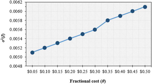
In performing lead time variance reduction, the vendor will be incurred a fractional cost of θ of the capital investment per unit time. In this section, we provide a simple analysis to investigate the effect of higher θ on the investment decision to be made by the vendor. The result of sensitivity analysis of change of value θ to model’s optimal solution is summarized in Table 4.

Table 4. Effects of different θ on the model’s optimal solution

θ	q* (units)	k*	σ ^2 (I)*	n* (shipments)	TCV	TCB	EJTC
$0.05	217	1.584	0.0051	2	$3,764.00	$1,511.60	$5,275.50
$0.10	217	1.583	0.0052	2	$3,799.30	$1,515.50	$5,314.70
$0.15	217	1.583	0.0053	2	$3,826.80	$1,519.40	$5,346.10
$0.20	217	1.582	0.0054	2	$3,849.10	$1,523.40	$5,372.40
$0.25	218	1.582	0.0055	2	$3,867.50	$1,527.30	$5,394.80
$0.30	218	1.581	0.0056	2	$3,882.70	$1,531.40	$5,414.10
$0.35	218	1.581	0.0058	2	$3,895.30	$1,535.40	$5,430.70
$0.40	218	1.580	0.0059	2	$3,905.50	$1,539.60	$5,445.10
$0.45	219	1.580	0.006	2	$3,913.60	$1,543.70	$5,457.30
$0.50	219	1.579	0.0061	2	$3,919.80	$1,548.00	$5,467.80

As θ increases, the value of σ ²(I) will also increase (see Figure 3). In this case, higher value of σ ²(I) indicates the system has worse lead time variance. The higher the fractional cost of θ causes the investment cost required to reduce the lead time variance becomes greater. Therefore, for the same amount of investment, the system will obtain a smaller reduction of lead time variance. On the other hand, an increase in the value of θ changes the decision regarding the shipment lot size and the service level offered by the company. The higher value of θ causes the optimal lot size to be larger, and the optimal service level to be lower. The expected joint total cost for the vendor–buyer system increases along with the increase in the value of θ.

Figure 3. Effects of different θ on σ ²(I).

5.3. Effects of b on model’s optimal solution

Parameter b refers to the coefficient of reduction for the function of I(σ ²). In this section, we observe the effects that parameter b gives to the model’s optimal solution regarding the investment decision σ ²(I). Table 5 presents the result from different values of b on the model’s optimal solution.

Table 5. Effects of different b on the model’s optimal solution

b	q* (units)	k*	σ ^2 (I)*	n* (shipments)	TCV	TCB	EJTC
0.0025	217	1.583	0.0053	2	$3,821.7	$1,518.6	$5,340.3
0.0030	217	1.583	0.0052	2	$3,809.1	$1,516.8	$5,325.9
0.0035	217	1.583	0.0052	2	$3,799.3	$1,515.5	$5,314.7
0.0040	217	1.584	0.0052	2	$3,791.3	$1,514.5	$5,305.8
0.0045	217	1.584	0.0052	2	$3,784.8	$1,513.7	$5,298.5
0.0050	217	1.584	0.0051	2	$3,779.3	$1,513.1	$5,292.4
0.0055	217	1.584	0.0051	2	$3,774.6	$1,512.7	$5,287.3
0.0060	217	1.584	0.0051	2	$3,770.6	$1,512.2	$5,282.8
0.0065	217	1.584	0.0051	2	$3,767.1	$1,511.9	$5,279.0
0.0070	217	1.584	0.0051	2	$3,764.0	$1,511.6	$5,275.5

As b increases, the value of σ ²(I) will slightly decrease. Yet, it does not change the optimal solution of q, k and n. For higher value of b, the system will experience a slight decrease in EJTC from the side of the vendor. Therefore, we conclude that different value of b will not affect the solution of the model significantly.

5.4. Effects of d on model’s optimal solution

This study considers a deterministic demand with a known and constant rate per year. In order to help the decision maker to deal with demand uncertainties in real case, we provide a simple sensitivity analysis regarding changes in demand and observe the behaviour of the model’s optimal solution of such changes. Tables 6 and 7 sum up the result from different values of D on the model’s optimal solution for Scenario I and II, respectively.

Table 6. Effects of different D on the model’s optimal solution for Scenario I

D (units/year)	q* (units)	k*	n* (shipments)	TCV	TCB	EJTC
1,000	225	1.56	2	$3,697.90	$1,665.80	$5,363.70
1,200	250	1.60	2	$4,269.60	$1,934.90	$6,204.50
1,400	272	1.64	2	$4,829.10	$2,199.60	$7,028.80
1,600	235	1.58	3	$5,338.70	$2,457.80	$7,796.50
1,800	219	1.53	4	$5,814.40	$2,724.00	$8,538.30
2,000	239	1.53	4	$6,261.90	$2,966.20	$9,228.10
2,200	235	1.48	5	$6,657.40	$3,219.00	$9,876.40
2,400	240	1.42	6	$7,008.40	$3,462.60	$10,471.00
2,600	244	1.29	8	$7,284.50	$3,707.30	$10,992.00
2,800	264	1.10	11	$7,450.30	$3,943.20	$11,393.00

Table 7. Effects of different D on the model’s optimal solution for Scenario II

D (units/year)	q* (units)	k*	n* (shipments)	σ^2(I)	TCV	TCB	EJTC
1,000	225	1.56	2	0.0052	$3,697.90	$1,665.80	$5,363.70
1,200	250	1.60	2	0.0052	$4,269.60	$1,934.90	$6,204.50
1,400	272	1.64	2	0.0051	$4,829.10	$2,199.60	$7,028.80
1,600	235	1.58	3	0.0051	$5,338.70	$2,457.80	$7,796.50
1,800	219	1.53	4	0.0051	$5,814.40	$2,724.00	$8,538.30
2,000	239	1.53	4	0.0051	$6,261.90	$2,966.20	$9,228.10
2,200	235	1.48	5	0.0051	$6,657.40	$3,219.00	$9,876.40
2,400	240	1.42	6	0.0051	$7,008.40	$3,462.60	$10,471.00
2,600	244	1.29	8	0.0051	$7,284.50	$3,707.30	$10,992.00
2,800	264	1.10	11	0.0051	$7,450.30	$3,943.20	$11,393.00

For both Scenario I and II, the increase in demand will eventually change the optimal solution of shipment lot size (q*), safety factor (k*) and number of shipments (n*). When the annual demand increases, shipment lot size and number of shipment will also increase. This result has implication on the holding cost, ordering cost as well as delivery cost per year. Therefore, an increase in demand will lead to an increase in the expected joint total cost per year of the vendor–buyer system. On the other hand, an increase in demand will cause the optimal safety factor k to decrease. Higher demand, at the same production rate, will reduce the system’s ability to meet the demand, which causes the optimal value of k to be decreased. However, the changes in D do not affect the decision regarding the optimal lead time variance reduction. For any number of demand each year, the optimal decision related to the lead time variance reduction will remain the same. Hence, we understand that uncertainties in demand will only affect decisions of q, n and k and do not change the decision regarding σ ²(I).

6. Conclusions

This research develops an integrated inventory model for a system of single-vendor single-buyer considering imperfect production process and investment for lead time variance reduction. The objective of this study is to minimize the expected joint total cost between the vendor and buyer. Several decision variables are included in the model, namely lot size, safety factor, target lead time variance and number of shipments from the vendor to the buyer. We propose an iterative procedure to solve the optimization problem. However, the result only ensures a local optimal solution and has not been able to guarantee a global optimal solution.

The results of this study show that the investment to reduce lead time variance will improve the system in terms of its ability to meet the demand and expected joint total cost per year. Thus, we conclude that investment policy is proved to give better outcomes to the system. We conduct a simple sensitivity analysis to study the effect of parameter changes on model’s optimal solution. Based on the results, we understand that an increase in the defective items proportion will significantly escalate the expected joint total cost of the system, whereas fractional cost of investment and coefficient of investment actually affect decisions related to lead time variance reduction and total expected total cost of the vendor–buyer system. Variation in demand influences the optimal shipment lot size, number of shipment, as well as safety factor. However, changes in demand do not change the optimal decision regarding lead time variance reduction.

The model proposed in this paper has several limitations that should be addressed in future studies. In our model, there is an assumption that vendor’s money is always available and sufficient to conduct the investment to reduce lead time variance. In practice, however, the money owned by the vendor to support the lead time investment may be limited. To accommodate this condition, the next model can be extended by considering the budget limitation. Later, the proposed model considers a simple supply chain system consisting of a vendor and a buyer. In reality, the structure of supply chain would be more complex. The supply chain may consist of vendor and multi-buyer. By assuming that the buyers have a willingness to support the vendor’s investment, the model can be further developed to determine the optimal distribution of buyer’s donation/payment. The extension of the study can also be done by investigating an inspection process. The proposed model assumes that the inspection process conducted by the buyer is perfect. The inspection process may be influenced by human error. The inspector may classify the good items as defective or classify the defective items as non-defective. Thus, incorporating both imperfect inspection and imperfect quality to vendor–buyer model would be more realistic for industrial setting.

Additional information

Funding

The authors received no direct funding for this research.

Notes on contributors

Wakhid Ahmad Jauhari

Wakhid Ahmad Jauhari is currently a lecturer in Universitas Sebelas Maret. He obtained bachelor and master degrees, both in industrial engineering, from Sepuluh Nopember Institute of Technology (ITS) in Surabaya, Indonesia. His research interests include modelling inventory, supply chain management and manufacturing design.

Mariana Sianipar

Mariana Sianipar is a junior researcher in in Production System Laboratory, Universitas Sebelas Maret. Her research interests are inventory management, logistic management and operation research.

Cucuk Nur Rosyidi

Cucuk Nur Rosyidi is a lecturer in Industrial Engineering Department of Universitas Sebelas Maret. His doctoral degree was obtained from Institut Teknologi Bandung Indonesia in the field of Manufacturing Systems in 2010. His research interests include product design and development, quality engineering and system modelling.

Anindya Rachma Dwicahyani

Anindya Rachma Dwicahyani is currently a lecturer in Universitas Jenderal Soedirman. Her research interests are inventory management, production management and operations research.

References

- Bala, K. (2014). Supply chain management: Some issues and challenges - A review. International Journal of Current Engineering and Technology , 4(2), 946–953.
- Banarjee, A. (1986). A joint economic-lot-size model for purchaser and vendor. Decision Sciences , 17(3), 292–311. doi:10.1111/j.1540-5915.1986.tb00228.x
- Chaharsooghi, S. K. , & Heydari, J. (2010). LT variance or LT mean reduction in supply chain management: Which one has a higher impact on SC perfomance? International Journal of Production Econom ics, 124(2), 475–481. doi:10.1016/j.ijpe.2009.12.010
- Dey, O. , & Giri, B. C. (2014). Optimal vendor investment for reducing defect rate in a vendor-buyer integrated system with imperfect production process. International Journal of Production Econom ics, 155, 222–228. doi:10.1016/j.ijpe.2014.02.004
- Ganeshan, R. , Kulkarni, S. , & Boone, T. (2001). Production economics and process quality: A taguchi perspective. International Journal of Production Econom ics, 71, 343–350. doi:10.1016/S0925-5273(00)00130-4
- Goyal, S. K. (1976). An integrated inventory model for a single supplier-single customer problem. International Journal of Production Research , 15(1), 107–111. doi:10.1080/00207547708943107
- Goyal, S. K. (1988). A joint economic-lot-size model for purchaser and vendor: A comment. Decision Sciences , 19(1), 236–241. doi:10.1111/deci.1988.19.issue-1
- Hamontree, C. , Ouelhadj, D. , & Beullens, P. (2012). Coordination buyer-supplier in supply chain models from net present value perspective. Lecture Notes in Management Science , 4, 136–144.
- Hayya, J. C. , Harrison, T. P. , & He, X. J. (2011). The impact of stochastic lead time reduction on inventory cost under order crossover. European Journal of Operational Research , 211, 274–281. doi:10.1016/j.ejor.2010.11.025
- Hoque, M. A. (2011). An optimal solution technique to the single-vendor multi-buyer integrated inventory supply chain by incorporating some realistic factors. European Journal of Operational Research , 215, 80–88. doi:10.1016/j.ejor.2011.05.036
- Jauhari, W. A. (2014a).). Integrated inventory model for single –Vendor single – Buyer with imperfect production process. International Journal of Operational Research , 20(3), 283–300. doi:10.1504/IJOR.2014.062451
- Jauhari, W. A. (2014b). Cooperative inventory model for vendor-buyer system with unequal-sized shipment, defective items and carbon emission cost. International Journal of Logistics Systems and Management , 10(2), 163–186. doi:10.1504/IJLSM.2014.064657
- Jauhari, W. A. (2018). A collaborative inventory model for vendor-buyer system with stochastic demand, defective items and carbon emission cost. International Journal of Logistics Systems and Management , 29(2). doi:10.1504/IJLSM.2018.089173
- Lee, J. S. , & Park, K. S. (1991). Joint determination of production cycle and inspection intervals in a deteriorating production system. Journal of Operational Research Society , 42(9), 775–783. doi:10.1057/jors.1991.148
- Lin, H. (2016). Investing in lead-time variability reduction in a collaborative vendor – Buyer supply chain model with stohchastic lead time. Computers & Operations Research 43–49).
- Lin, T. Y. (2010a). An economic order quantity with imperfect quality and quantity discounts. Applied Mathematical Modelling , 34, 3158–3165. doi:10.1016/j.apm.2010.02.004
- Lin, Y. (2010b). A stochastic periodic review integrated inventory model involving defective items, backorder price discount, and variable lead time. 4OR, 8, 281–297.
- Lo, C. (2013). A collaborative business model for imperfect process with setup cost and lead time reductions. Open Journal of Social Sciences , 6–11. doi:10.4236/jss.2013.17002
- Nasri, F. , Paknejad, J. , & Affisco, J. (2008). Investing in lead-time variability reduction in a quality-adjusted inventory model with finite-range stochastic lead time. Journal of Applied Mathematics and Decision Sciences , 2008, 1–13. doi:10.1155/2008/795869
- Paknejad, M. J. , Nasri, F. , & Affisco, J. F. (1992). Lead-time variability reduction in stochastic inventory models. European Journal of Operational Research , 62, 311–322. doi:10.1016/0377-2217(92)90121-O
- Porteus, E. L. (1986). Optimal lot sizing, process quality improvement and setup cost reduction. Operation Research , 34(1), 137–144. doi:10.1287/opre.34.1.137
- Sajadieh, M. , & Larsen, C. (2015). A coordinated manufafacturer-retailer model under stochastic demand and production rate. International Journal of Production Economics , 168, 64–70. doi:10.1016/j.ijpe.2015.06.013
- Sana, S. S. (2010). A production-inventory model in an imperfect production process. European Journal of Operational Research , 200, 451–464. doi:10.1016/j.ejor.2009.01.041
- Simchi-Levi, D. , Kaminsky, P. , & Simchi-Levi, E. (2008). Designing and managing the supply chain: Concepts, strategies, and case studies . Irwin: McGraw-Hill.