VLCC’s fuel consumption prediction modeling based on noon report and automatic identification system

Abstract

It is extremely important for fuel saving by taking the correct decisions where cost efficiency and environmental friendliness are top priorities. The fuel consumption rate of the ship is influenced by many parameters, such as average daily sailing speed, ship displacement, cargo, ballast water and bunker, trim and sea conditions (wind, wave and current) in a complicated way. In this study, noon report (NR) and automatic identification system (AIS) datum of four Very Large Crude Carriers (VLCC) are widely used to establish a prediction model. Needless to say that, the accuracy of statistical models depends on consistency and quality of collected datum, hence a novel combination methodology applied to NR and AIS datum to prepare a series of pure valid data population of vessel speed, fuel consumption and sea state. Then the consistency of populations are enriched by eliminating the out ranged or junkie members in different methods, i.e., T-test, normality control and outlier score base (OSB).

Finally, multiple linear regressions are applied considering all fuel consumption influential parameters. Results show a high correlation between the independent and dependent variables. Consequently, generated formula predicts fuel consumption of vessels at all variable conditions in good agreement with recorded fuel consumption data.

Keywords:

• fuel consumption
• sea state
• multiple linear regressions
• noon report data
• automatic identification system
• VLCC

PUBLIC INTEREST STATEMENT

Since the fuel consumption costs is the most considerable item among all ship operational and voyage cost elements, all ship owners are so concerns about reduction of this item in an envisaged voyage. One of the approach in reducing this cost in ship owners point of view is to predict the fuel consumption in each voyage precisely taking into consideration other influential factors such as sea condition. This paper presents a practical prediction formula based on the data collected and reported to the owners on daily basis for Very Large Crude Carrier (VLCC). It helps the owners not only to predict their yearly budget for fuel consumption and prevent any unwanted element resulting in increasing the fuel consumption but also to enable owners to decrease the consumption because of his full awareness on the real influential factors affecting the fuel consumption in each voyage. In addition, the paper presents an economical parcel size to be loaded in regard to maximizing owner income for the voyage.

1. Introduction

Fuel consumption rate of a ship is influenced by many parameters, such as average daily sailing speed, weight of ship, cargo, ballast water and bunker; trim and sea conditions (wind, wave and current) in a complicated way. So far, many researchers investigated on reducing fuel consumption.

After significant increase in fuel price in 2008, onboard ships, commonly referred to as “bunkers”, has become the largest cost item of a ship’s operational expenses, accounting today almost 50% of a voyage cost, even greater than crew wages (Stopford, 2009). The level of interest in designing a fuel efficient ship is linearly related to the fuel price. Between 1970 and 1980 fuel oil price increased significantly (nearly ten-fold), leading to ships with high fuel consumption being laid up (Wijnolst & Wergeland, 2009). During the period 1985–2000 prices of fuel oil fell, with research and development on energy efficiency not receiving particular attention by the maritime industry. However, from year 2000 the crude oil cost started to climb again, which pushed engine manufacturers, shipyards and designers to re-investigate design and operational solutions for reducing fuel consumption and increasing energy efficiency. Shipping is no different than other industries, and is highly affected by fuel prices. However, there is, to a certain extent, a control on the ship’s fuel consumption by means of technical innovation fitted or by better ship operation such as weather routing, trimming, slow steaming, etc. (DNV, 2010). Even though oil price decreased for a brief period of time after the 2008 recession, today is again at record high levels, meaning that ship operators cannot ignore this expense as in the past, or just embody it into the price of the commodities carried, but there is a need to design and operate more efficient ships, consuming less fuel per carrying capacity. Furthermore, the intense focus on environmental protection, supported by considerable research findings, has led the international maritime organization (IMO) to take concerted measures towards this direction, in limiting the environment foot print of ships significantly. In particular, one of the top environmental topics is global warming due to increasing greenhouse gases (GHG) in the atmosphere. The shipping industry contributed about 4% of the world carbon dioxide (CO₂) emissions in 2007 (Reynolds, 2009). The aim is to reduce CO₂ emissions comes hand in hand with the increasing fuel price, and is leading towards the adoption of technological and operational innovations in order to decrease fuel consumption. In order to set means to improve ship’s fuel efficiency, it is initially required to define the prevailing fuel consumption rate. For this purpose, the importance of carrying out a full scale ship performance analysis is highlighted in several publications as offering benefits to the designers and the operators. The aim of such an analysis can, for example, be the prediction of the required propulsion power (Pedersen & Larsen, 2009), or monitoring of the hull resistance due to fouling (Aas-Hansen, 2011). Boom et al. suggested that since sensors are already found onboard along with equipment to transmit the information, continuous monitoring may be achieved with adequate analysis (Boom, Koning, & Aalbrets, 2005). Coraddu et al. after collecting needed data on-board, created a data analytics method to calculate vessel fuel consumption. They declared that the latter can be used to reduce the vessel consumption by means of optimizing the vessel operational conditions. In particular, they have shown that gray-box models (GBM) are able to combine the high prediction accuracy of black-box models (BBM) while reducing the amount of data required for training the model by adding a white-box model (WBM) component. The resulting GBM model is then used for optimizing the trim of the vessel, suggesting that between 0.5 and 2.3% fuel savings can be obtained by appropriately trimming the ship, depending on the extent of the range for varying the trim (Coraddu, Oneto, Baldi, & Anguita, 2006). Henggeler, Henry, and Kenny (n.d.) proposed chart base correlations to estimate energy efficiency by measuring diesel fuel consumption. In 7th Society of Arctic Climate Change, Economy and Calculation of fuel consumption per mile for various ship types and ice conditions in past, present and in future has been studied. It has stated that there is no unambiguous relation between ice situation (extent, thickness, coverage) and the fuel consumption and exhaust emission. The reason is that if the ice extent increases towards the winter period fewer ships are able to travel the northern routes in a reasonable time. Additionally in the intermediate periods (freeze up and melting) ships will be restricted in speed due to safety reasons. In order to accumulate exhausts emissions for the arctic region for future times the number of ships, which may operate under reasonable safe and economic conditions, has to be determined. This number will be depending on the development of the region and its infrastructure (socio economic factors). Moreover, the travel time and operation condition of the different ship types will be of major concern as the speed profile will not only depend on technical ability but on freight rates and type of goods to be transported along the northern sea route (7th Arctic Climate Chang Economy and Society, 2014). Donggon (2016) has studied the economic impact of fuel consumption uncertainty for tankers as M.Sc. thesis. According to his published study empirical results show that optimal speed is very sensitive to bunker price rather than freight when subject to various weather and hull fouling conditions. The economic impact of uncertainty in weather and hull fouling conditions has not been empirically estimated on the basis of detailed noon report (NR) data. In this regard, as the first attempt he analyzed various factors in real life ship operation change the decision making for profit maximization and speed optimization. Bialystocki and Konovessis (2016) proposed a statistic method for prediction of fuel consumption procedure as shown in Figure 1. It illustrates the algorithm developed for the prediction of fuel consumption and speed curve. By utilizing the correlation curve, it is possible to estimate the fuel consumption in a future voyage, based on predetermined information. Initially, three corrections are applied before a preliminary curve is plotted:

1. The ground speed was calculated by dividing the traveled main distance with the steaming time. More so, the engine fuel consumption is per steaming time. Therefore, fuel consumption is corrected.

2. Departure and arrival drafts for each voyage were also recorded, and intermediate ship’s drafts were calculated using interpolation. Thereafter, a correction to the fuel consumption of the actual draft to design draft is carried out using the Admiralty coefficient.

3. Ground speed was corrected to take into consideration the current, if occurred. When the current flowed aft wards it was added to the ground speed, while in case that the current flowed forward it was deducted from the ground speed.

Figure 1. Statistic method’s chart for prediction of fuel consumption

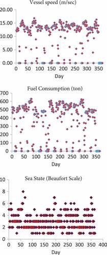
As mentioned, some required data are collected from NR and AIS for VLCC. These data are used for establishing reliable equations to predict fuel consumption. NR data is found in by chief officer or captain of the ship once a day. Always human error is a part of all reports made by human. Therefore, when reviewing NR data, it is often found that some data are odd and not in right harmony with the others. There are many statistical methods to find the roots of the data’s harmonies or odd data. In order to acquire pure valid NR data for defining thoroughly relation between the tankers fuel consumption influential parameters, the NR data of four VLCC ships are composed with their respective AIS data. Then, the out ranged or junkie’s data are determined by different methods, i.e., T-test, normality control and OSB. Furthermore, the outlier scour based method used for filtering data to enhance better correlation between parameters (Safaei, Ghassemi & Ghiasi, 2018, 2019). The formula proposed may be used for prediction of fuel consumption taking into consideration the independent and dependent variables including ship speed, ship displacement, trim, sea state and fuel consumption rates. Figure 2–5 show the raw data of the vessel speed, fuel consumption and sea states for four ships (DUNE, DIONA, SEASTAR III, SERENA).

Figure 2. Ship 1 (DUNE)

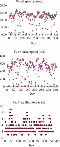
Figure 3. Ship 2 (DIONA)

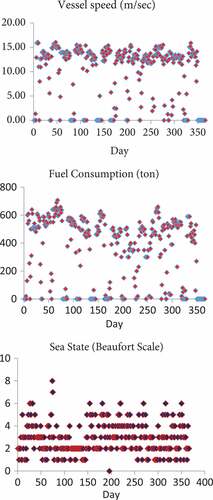
Figure 4. Ship 3 (SEASTAR III)

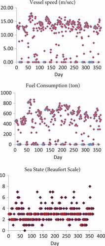
Figure 5. Ship 4 (SERENA)

2. Prediction methods

Durbin–Watson test performed to validate the independency of all variables. This well-known method is applicable for inferential suitability models with serious deficiency in serial correlation (e.g., assessing the confidence in the predicted value of a dependent variable). On the other hand, the method is able to find multi variable correlation by fewer complexity in order to its linear nature. Also superposition rule can be deployed to use more correlated variables. The test statistic of the Durbin–Watson procedure is d and is calculated as follows (O’Brien, 2007):

(1) $\mathrm{d}=\frac{{\sum }_{\mathrm{t}=2}^{\mathrm{n}}{\left({\mathrm{e}}_{\mathrm{t}}-{{\mathrm{e}}_{\mathrm{t}}}_{-1}\right)}^2}{{\sum }_{\mathrm{t}=1}^{\mathrm{n}}{\mathrm{e}}_{\mathrm{t}}^2}$(1)

Recall that e_t represents the observed error term (i.e., residuals) or:

(2) $\left({\mathrm{Y}}_{\mathrm{t}}-{\hat{Y}}_{\mathrm{t}}\right)={\mathrm{Y}}_{\mathrm{t}}-\mathrm{a}-\mathrm{b}\ast {\mathrm{X}}_{\mathrm{t}}$(2)

It can be shown that the value of $\mathrm{d}$ will be between zero and four; zero corresponding to perfect positive correlation and four to perfect negative correlation. If the error terms, e_t and $\mathrm{e}\mathrm{t}-1$, are uncorrelated, the expected value of d is two. When the calculated value of d is less than two, it shows the independent variables have first order serial correlation otherwise they have nonlinear or parallel relation. Unfortunately, the Durbin–Watson test can be inconclusive. As a general rule if d value be between 1.5 and 2.5, the independency of variables would be satisfactory. The variables in this essay are defined as follows:

• Fc: Fuel consumption (tons/day)

• Ds: Ship displacement (metric tons)

• Vv: Ship velocity (k)

• Wv: Wave height (Beaufort scale)

• Wn: Wind speed (Beaufort scale)

The results of Dubin Watson test for variables have presented in Table 1.

Table 1. Durbin–Watson test results for${\mathbf{W}}_{\mathbf{n}},{\mathbf{V}}_{\mathbf{v}},{\mathbf{D}}_{\mathbf{s}}$and ${\mathbf{W}}_{\mathbf{v}}$

Model	R	R^2	Adjusted R^2	Durbin–Watson
1	0.868	0.753	0.752	1.306

The d value calculated for four parameters${\mathrm{W}}_{\mathrm{n}},{\mathrm{V}}_{\mathrm{v}},{\mathrm{D}}_{\mathrm{s}}$ $\mathrm{a}\mathrm{n}\mathrm{d}{\mathrm{W}}_{\mathrm{v}}$is about 1.3 that shows correlation between variables. The other test done by ignoring ${\mathrm{W}}_{\mathrm{n}}$ (because of probability of correlation between ${\mathrm{W}}_{\mathrm{v}}$ and ${\mathrm{W}}_{\mathrm{n}}$). The results are presented in Table 2. By ignoring ${\mathrm{W}}_{\mathrm{n}}$, the d value becomes 1.67 that shows the regression can done based on variables.

Table 2. Durbin–Watson test results for $,{\mathbf{V}}_{\mathbf{v}},{\mathbf{D}}_{\mathbf{s}}$and ${\mathbf{W}}_{\mathbf{v}}$

Model	R	R^2	Adjusted R^2	Durbin–Watson
1	0.865	0.748	0.747	1.67

Table 3 shows the results of co-linearity control of independent variables. A tolerance of less than 0.20 or 0.10 and/or a variance inflation factor (VIF) of 5 or 10 and above indicates a co-linearity problem (O’Brien, 2007). As evident in the table, wave and wind parameters have significant co-linearity with other independent variables. So the correlation of independent variables shall check pairwise.

Table 3. Co-linearity control results

Model	Unstandardized coefficients		Standardized coefficients	Collinearity statistics
	B	Std. error	Beta	Tolerance	VIF
(Constant)	−298.676	19.366
${\mathrm{D}}_{\mathrm{s}}$	1.469	0.040	0.704	0.659	1.518
${\mathrm{V}}_{\mathrm{v}}$	20.026	1.633	0.227	0.694	1.440
${\mathrm{W}}_{\mathrm{v}}$	−14.052	4.500	−.160	0.090	11.152
${\mathrm{W}}_{\mathrm{n}}$	20.631	4.386	0.240	0.091	11.023

In the second step, the Pearson’s correlation coefficient is calculated for data sets. This coefficient often referred to as the Pearson’s R test is a statistical formula that measures the strength between variables and relationships. To determine how strong the relationship is between two variables, it is needed to find the coefficient value, which can range between −1 and +1. The results of Pierson test are shown in Table 4. It is evident from Table 4 that there is a significant correlation between wind and wave and ignoring one of these two variables can lead to better regression results. So according to orientation consideration, the wind effect has been ignored in regression.

Table 4. Correlations between variables based on Pierson test

Pearson’s correlation	Parameter	FC	Ds	Vv	Wv	Wn
	FC	1.000	0.842	0.604	0.231	0.253
	Ds	0.842	1.000	0.530	0.237	0.233
	Vv	0.604	0.530	1.000	−0.017	0.006
	Wv	0.231	0.237	−.017	1.000	0.953
	Wn	0.253	0.233	0.006	0.953	1.000

The Breusch–Pagan (BP) test is one of the most common tests for heteroscedasticity. It begins by allowing the heteroscedasticity process to be a function of one or more of your independent variables, and it is usually applied by assuming that heteroscedasticity may be a linear function of all the independent variables in the model. This assumption can be expressed as follows:

(3) ${\epsilon }_{\mathrm{i}}^2={\alpha }_0+{\alpha }_1{\mathrm{X}}_{\mathrm{i}1}+\dots +{\alpha }_{\mathrm{p}}{\mathrm{X}}_{\mathrm{i}\mathrm{p}}+{\mathrm{u}}_{\mathrm{i}}$(3)

The values for ${\epsilon }_{\mathrm{i}}^2$ are not known in practice, so ${\hat{\epsilon }}_{\mathrm{i}}^2$ are calculated from the residuals and used as proxies for ${\epsilon }_{\mathrm{i}}^2$. Generally, the BP test is based on the estimation of:

(4) ${\hat{\epsilon }}_{\mathrm{i}}^2={\alpha }_0+{\alpha }_1{\mathrm{X}}_{\mathrm{i}1}+\dots +{\alpha }_{\mathrm{p}}{\mathrm{X}}_{\mathrm{i}\mathrm{p}}+{\mathrm{u}}_{\mathrm{i}}$(4)

Alternatively, a BP test can be performed by estimating:

(5) ${\hat{\epsilon }}_{\mathrm{i}}^2={\delta }_0+{\delta }_1\widehat{{\mathrm{Y}}_{\mathrm{i}}}$(5)

where $\hat{\mathrm{Y}}$ represents the predicted values from:

(6) $\widehat{{\mathrm{Y}}_{\mathrm{i}}}=\widehat{{\beta }_0}+\widehat{{\beta }_1}{\mathrm{X}}_{\mathrm{i}1}+\dots +\widehat{{\beta }_{\mathrm{p}}}{\mathrm{X}}_{\mathrm{i}\mathrm{p}}$(6)

So in this study estimation of model performed using ordinary least-squared (OLS):

(7) ${\mathrm{Y}}_{\mathrm{i}}={\beta }_0+{\beta }_1{\mathrm{X}}_{\mathrm{i}1}+\dots +{\beta }_{\mathrm{p}}{\mathrm{X}}_{\mathrm{i}\mathrm{p}}+{\epsilon }_{\mathrm{i}}$(7)

The predicted Y values were obtained after estimating the model then Estimation of the auxiliary regression performed using OLS:

(8) ${\hat{\epsilon }}_{\mathrm{i}}^2={\delta }_0+{\delta }_1\widehat{{\mathrm{Y}}_{\mathrm{i}}}$(8)

The R² value retained from the auxiliary regression ${\mathrm{R}}_{{\bar{\mathrm{S}}}^2}^2.$Finally, F-statistic or the chi-squared statistic is calculated as follows:

(9) $\mathrm{F}=\frac{\frac{\mathrm{R}\frac{2}{{\mathrm{s}}^2}}{1}}{\frac{\left(1-\mathrm{R}\frac{2}{{\mathrm{s}}^2}\right)}{\mathrm{n}-2}}\mathrm{o}\mathrm{r}{\mathrm{X}}^2=\mathrm{n}\mathrm{R}\frac{2}{{\mathrm{s}}^2}$(9)

3. Result

The degrees of freedom for the F-test are equal to 1 in the numerator and n–2 in the denominator. The degrees of freedom for the chi-squared test are equal to 1. If either of these test statistics is significant, then you have evidence of heteroscedasticity. If not, you fail to reject the null hypothesis of homoscedasticity. The result of BP test is presented in Table 5.

Table 5. Breusch–Pagan test results

Breusch–Pagan/Cook–Weisberg test for heteroskedasticity

Ho: Constant variance

Variables: Ds Vv Wv

Chi^2(3) = 3.24 Prob > chi^2 = 0.0921

As shown in Table 5, the P-value is more than 0.05 so the null hypothesis did not reject so the variables have homoscedasticity and multiple linear regressions can be done.

For this issue, stepwise method is performed. The results are presented in Table 6.

Table 6. Multiple linear regression (stepwise method) results

	Model	Unstandardized coefficients		t	Sig.
		β	Std. e
1	(Constant) Ds	−87.824	12.284	−7.149	0
		1.757	.035	50.474	0
2	(Constant) Ds Vv	−266.518	18.994	−14.032	0
		1.515	.039	39.289	0
		19.353	1.634	11.844	0
3	(Constant) Ds Vv Wv	–$1393$	19.349	−14.745	0
		$0.001$	.040	36.680	0
		$116.6$	1.645	12.497	0
		$4.94$	1.422	4.257	0

By performing the regression on the variables in final model (Model No. 3), it is obtained from significance coefficient values that there is significant relation between independent variables and Fuel Consumption also the β coefficient shows all the independent variables have positive effect on fuel consumption.

The predicted formula will be as follows:

(10) $F_c=-1393+116.6Vv+0.001Ds+4.94Wv$(10)

For example, the fuel consumption in the case of 5 continuous days calculated by the formula and compared with NR data are tested. The results show the accuracy of prediction is about 97% in those days. The results are presented in Table 7.

Table 7. Comparing the fuel consumption predicted by formula and recorded data in the noon reports (report is given just for 5 days)

Day	Ds	Vv	Wv	FC Recorded in the noon reports	FC p by formula	Formula accuracy
1	334.08	12.43	3	70	70.28	97.8%
2	342.89	12.42	2	64.10	64.18	97%
3	353.60	12.38	3	64.4	63.3	98%
4	205.55	12.37	5	73.3	72.88	99%
5	318.96	12.34	2	54.9	54.86	97%

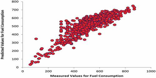
Figure 6 depicts the predicted for the fuel consumption versus measured values for all four VLCC’s ships. The voyage for all ships was from Khark Island heading laden to one south Chinese port. As it is shown, all data are in great accuracy with reported fuel consumptions.

Figure 6. Predicted and measured values of fuel consumption for all ships

4. Conclusion

In this study, some raw data of fuel consumption, speed, sea states are collected from NR and AIS for four VLCC ships. These data are analyzed in order to acquire a pure valid NR data for defining thoroughly relation between the tankers fuel consumption influential parameters by taking the following steps. In the first step, the NR data of four VLCC ships are composed with their respective AIS data and then the out ranged or junkie’s data are determined by different methods, i.e., T-test, normality control and OSB.

By perfuming the regression, the prediction formula produced indicating a high correlation between independent variables (ship speed, displacement, wind and sea states) and dependent variables (fuel consumption). The calculated R² value for estimating the accuracy of the model is about 0.75; therefore, independent variables can be predicted 75% of variation of fuel consumption. According to proposed model, by step-wise regression, ship speed has the greatest coefficient in the equation. Afterward wind and displacement coefficients are, respectively, 0.3 and 0.07 of ship speed impact. In future study, it is recommended to use nonlinear regression methods to increase the accuracy of the prediction due to the nonlinear physical relation of ship speed and fuel consumption.

Additional information

Funding

The authors received no direct funding for this research.

Notes on contributors

Ali Akbar Safaei

Ali Akbar Safaei is PhD student at Department of maritime Engineering, Amirkabir University of Technology. His thesis is on the fuel consumption of the marine vehicle transportation. In his 27 years of career, he has been chairing, managing director, general director and head of department for different shipping companies particularly oil tankers and ports authority.

Hassan Ghassemi

Hassan Ghassemi is a professor at Department of maritime Engineering, Amirkabir University of Technology. He published around 120 journal peer reviewed papers and 8 books. His major field is marine hydrodynamics and propulsion, CFD, BEM and Marine Renewable Energy. More detail may be found in http://hmaa.itgo.com/ghassemi.html.

Mahmoud Ghiasi

Mahmoud Ghiasi is an associate professor at Department of maritime Engineering, Amirkabir University of Technology. His major field is marine hydrodynamics, CFD and numerical modelling. He published many articles in the field of ship hydrodynamics and marine propulsion.

References

- 7th Arctic Climate Chang Economy and Society. (2014). Calculation of fuel consumption per mile for various ship types and ice condition in past, present and future. http://www.access-eu.org/modules/resources/download/access/Deliverables/D2-42-HSVA_Report_CE_CS_NR_rev02_submitted.pdf
- Aas-Hansen, M. (2011). Monitoring of hull condition of ships( Mater thesis). Norwegian University of Science and Technology, Norway.
- Bialystocki, N., & Konovessis, D. (2016). On the estimation of ship’s fuel consumption and speed curve: A statistical approach. Journal of Ocean Engineering and Science, 1, 157–12. doi:10.1016/j.joes.2016.02.001
- Boom, H. V. D., Koning, J., & Aalbrets, P. (2005, May). Proceedings of the offshore technology Conference (pp. 2–5), Huston, TX.
- Coraddu, A., Oneto, L., Baldi, F., & Anguita, D. (2006). Soft computing for sustainability science, studies in fuzziness and soft computing (pp. 358). Book series, Springer. doi:10.1007/978-3-319-62359-7
- DNV. (2010). Assessment of measures to reduce future CO2 emission from shipping, research and innovation (Position paper No. 5). Hovik: Det Norsk Veritas.
- Donggon, B. (2016). The economic impact of fuel consumption uncertainty for tankers ( Master thesis for the Master of Science in Economics and Business Administration within the main profile International Business). Norwegian School of Economics.
- Henggeler, J., Henry, C., & Kenny, N. (2009). Measuring diesel fuel consumption to estimate engine efficiency. http://crops.missouri.edu/irrigation/dieselconsumption.pdf
- O’Brien, R. M. (2007). A caution regarding rules of thumb for variance inflation factors. Quality & Quantity, 41(5), 673. doi:10.1007/s11135-006-9018-6
- Pedersen, B. P., & Larsen, J. (2009, January 21–24). Modeling of ship propulsion performance, Proceedings of the World Maritime Technology Conference. Mumbai, India: WMRC.
- Reynolds, G. (2009, January 21–24). Proceedings of the World Maritime Technology Conference WMRC. Mumbai: WMRC.
- Safaei, A. A., Ghassemi, H., & Ghiasi, M. (2018). Correcting and enriching vessel’s noon report data using statistical and data mining methods, European transport (pp. 67).
- Safaei, A. A., Ghassemi, H., & Ghiasi, M. (2019). New methodology for acquiring pure valid data by combining oil tankers’ noon report and automatic identification system satellite data using statistical and data mining methods. Journal PROMET – Traffic & Transportation.
- Stopford, M. (2009). Maritime economics (3rd ed.). Oxford: Routledge.
- Wijnolst, N., & Wergeland, T. (2009). Shipping innovation. Amsterdam: IOS Press.