Model for remaining strength estimation of a corroded pipeline with interacting defects for oil and gas operations

Abstract

Remaining strength estimation of corroded pipelines is a major consideration in pipeline integrity management. The loss of pipe wall thickness due to corrosion inevitably leads to a reduction in the pipeline’s strength and ability to sustain a design pressure. If corrosion defects are closely spaced, the corrosion feature may interact, resulting in failure pressure lower than would be expected if the defects were evaluated as separate flaws. In such a situation, industry methods for remaining strength calculation have been shown to be conservative. This present work presents a new model that improves the current methodologies for estimating the remaining strength of a corroded pipeline with interacting defects, utilizing a finite element analysis approach in combination with curve fitting. The new model demonstrates the potentials of improved estimation of the remaining strength over the existing industry models. The implication is that the presented model has the potentials of reducing the conservatism inherent in the existing models for estimating the remaining strength of oil and gas pipelines.

Keywords:

• remaining strength estimation
• corroded pipelines
• pipeline integrity management
• finite element analysis
• interacting defects
• oil and gas

PUBLIC INTEREST STATEMENT

Remaining strength estimation of corroded pipelines is a major consideration in pipeline integrity management. However, the industry methods for remaining strength calculation have been shown to be conservative. This paper presents an improved model for estimating the remaining strength of a corroded pipeline with interacting defects. The new model demonstrates the potentials of improved estimation of the remaining strength over the existing industry models for all cases of defects—shallow and deep defects. The implication is that the presented model has the potentials of reducing the conservatism inherent in the existing models for estimating the remaining strength of oil and gas pipelines.

1. Introduction

Oil and gas play an important role in the energy needs of modern society. However, in recent times, the oil and gas industry has witnessed a dwindling return, which calls for prudent management of oil and gas assets. Pipeline, as one of the oil and gas assets, has always been considered as the safest means of economically conveying petroleum products, namely oil, gas, liquefied natural gas, etc., across long distances and difficult terrains (Mohitpour, Golshan, & Murray, 2000). However, with age and usage come the effect of corrosion mechanisms, which impact the strength, integrity and pressure containment capability, and consequently, the reliability of pipeline systems (McAllister, 2000; Wang, Li, Chang, & Huang, 2016), and, therefore, such pipelines must be assessed to determine if they will continue in service and under what conditions (API 5L, 2004; ASME B31G, 2012).

There are a number of assessment methods currently used for fitness-for-service assessment of corroded pipelines, each having their own pros and cons (Amaya-Gómez, Sánchez-Silva, Bastidas-Arteaga, Schoefs, & Muñoz, 2019). The ASME B31G (2012) and the DNV RP-F101 (2010) are the two most commonly used standards; others include the modified B31G and the RSTRENG criteria, and many other proprietary models have also been developed, such as the FITNET FFS, SHELL 92, the British Gas Model, etc. (Bipul & Ashutosh, 2017; Dick & Inegiyemiema, 2014; Ossai, 2017). By using the abovementioned methods, the defects in a pipeline due to corrosion can be measured, and this may be determined with the use of nonestructive examination techniques ranging from visual, radiographic, ultrasonic and other methods of measurement and followed by calculation of remaining strength using the established criteria (Chanyalew, Mokhtar & Karuppanan, 2011).

However, not all imperfections due to corrosion could be regarded as defects according to some industry codes, namely ASME31.8 (2012) and API 5L (2004). ASME B31.8 (2012) defines a defect as any imperfection with dimensions or characteristics that exceed the acceptable limits under the code, whereas API 5L (2004) defines a defect as an imperfection of sufficient magnitude to warrant rejection of the product based on the stipulations of the applicable specification. Therefore, defect is relative to the code or specification under which an item is being assessed. ASME B31.8 defined defect assessment as a documented evaluation using engineering principles and the effects of relevant variables of a flaw in the service life or strength of the pipeline. Assessment provides a rational basis to ascertain if a flawed pipeline can continue in service or whether it must be repaired or replaced.

The methods outlined in the industry codes for the fitness-for-purpose assessment of corroded pipelines, such as the ASME B31G, DNV RP F101, RSTRENG, etc., are usually best suited for evaluating singular defects. However, if the defects are spaced closely, as shown in Figure 1 (adapted from Karuppanam, Aminidin & Wahab (2012)), the defects may interact with each other in such a way that they result in failure at a pressure much lower than would be anticipated based on the impact of the separate defects. Under the ASME B31G code, based on empirical observation, corrosion defects are considered to be interacting if the distance between them is less than or equal to three times the pipe wall thickness (3t). Interacting defects are to be evaluated to be one single defect, with the effective length adjudged to be the sum of all interacting flaws as shown in Figure 2. In the DNV (2010) code, close defects are only deemed to be interacting when the limit of the longitudinal distance between the defects is two times the square root of the product of the external diameter and thickness of pipe, ${\mathrm{s}}_{\mathrm{l}}=2.0\sqrt{\mathrm{D}\mathrm{t}}$, and when the limit of the circumferential distance between the defects is 3.142 times the square root of the product of the external diameter and thickness of pipe, ${\mathrm{s}}_{\mathrm{c}}=\pi \sqrt{\mathrm{D}\mathrm{t}}$.

Figure 1. Corrosion feature interaction

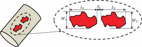
Figure 2. ASME B31G assumption for interacting defects (adapted from ASME B31G (2012))

Chanyalew, Mokhtar, and Karuppanan (2011) used the finite element analysis (FEA) to estimate the remaining strength of corroded in-service pipelines, which gives a more realistic prediction of pipeline failure under corrosion attack. The authors’ study observed that available industry codes for pipeline corrosion assessment are conservative, which could also be demonstrated by the results presented in Al-Owaisia et al. (2018). Finite element methods developed by Bipul and Ashutosh (2017) and that used by Ossai (2017) estimated both the failure pressure and applied safety factors needed to apply in modeling pipeline sections undergoing different rates of corrosion. The progressive corrosion growth was also simulated by the authors. Further studies, using the same method but for two interacting defects, developed a multiplication function by finding the ratio of normalize failure pressures and other failure parameters using the DNV code (Karuppanan, Aminidin, & Wahab, 2012). Though the authors have advanced the application of FEA in estimating the remaining strength of pipelines, the cases of interacting defects have not been fully studied. Therefore, the aim of this work is to improve the existing methods for the estimation of a corroded pipelines’ remaining strength for cases of interacting defects using a FEA and curve-fitting approach.

2. Material and methods

ANSYS FEA software was used to simulate selected cases of corrosion feature interaction on a pipeline section. The results from the FEA were used to modify the remaining strength (RSTRENG) formula for improved performance. This was achieved by the inclusion of a multiplication function obtained through curve fitting analysis.

2.1. Finite element analysis

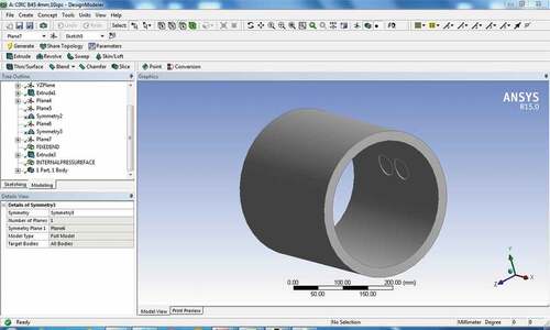
The pipe section, with two interacting defects, was modeled in the ANSYS FEA environment, as shown in Figure 3. The circular/spherical corrosion profile was considered as the near-approximation of the pitting corrosion found naturally in oil and gas pipelines.

Figure 3. Interacting defects model in ANSYS environment

Symmetry planes were also created in order to reduce the model to a quarter section of the entire pipe, which captures the corrosion pit profile as shown in Figure 4. This was to reduce computation time and Centre Processing Unit (CPU) requirement.

Figure 4. Model symmetry creation

Combination of triangular and tetrahedral mesh was used to enhance the accuracy of the results and closeness to real-life occurrence. Internal pressure load is applied to the model iteratively until failure, and the failure pressure recorded. Meshing and the load application are shown in Figure 5.

Figure 5. Meshing and load application

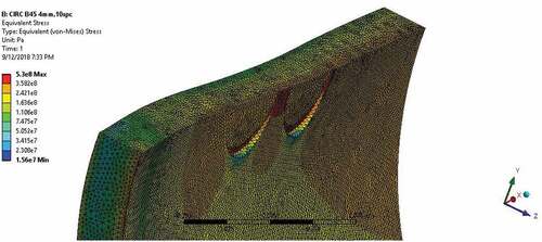
The setup for the simulations basically involved two independent variables (inputs), namely the inter-defects spacing, which ranged from 10 to 60 mm, and the defect depths which was varied from 4 to 14 mm, while the dependent variable or the output is the failure pressure. The pipe material yield strength is compared with Von Mises stress, and the pipe is considered to have failed once the Von Mises stress matches or surpasses the ultimate tensile strength of the pipe. Physical and material properties of the pipe section being modeled are presented in Table 1.

Table 1. Pipe section dimensions and material properties

Parameters	Values
Pipe type Pipe nominal diameter	API 5L$\times$65 steel 300 mm (NPS 12ʹ’)
Length of pipe section	300 mm
Pipe thickness	20 mm
Pipe density	7850 kg/m^3
Ultimate tensile strength	530 MPa
Yield strength	448 MPa
Young modulus	2.07 $\times$ ${10}^5$ MPa

2.2. Curve fitting

The corroded pipeline’s remaining strength was estimated as the ratio of the estimated failure pressure of the corroded pipe to the initial design pressure of the pipeline, which can be used as a direct measure of the pipeline’s remaining strength.

The failure/burst pressure for a corroded pipeline under the RSTRENG method can be calculated using Equation (1)(1) $P_f={\sigma }_s+68.95\ast \frac{2t}{D}\ast \left[\frac{1-0.85d/t}{1-0.85d/t\ast \frac{1}{M}}\right]$(1) ;

(1) $P_f={\sigma }_s+68.95\ast \frac{2t}{D}\ast \left[\frac{1-0.85d/t}{1-0.85d/t\ast \frac{1}{M}}\right]$(1)

where M, the Folias factor, is calculated according to Equation (2)(2) $M=\left\{\begin{array}{c}\sqrt{1+0.6257\left(\frac{L^2}{Dt}\right)-0.003375{\left(\frac{L^2}{Dt}\right)}^2},forL\le \sqrt{50Dt}\\ \hspace{0.17em}\\ 3.3+0.032\frac{L^2}{Dt},forL>\sqrt{50Dt}\end{array}\right.$(2)

(2) $M=\left\{\begin{array}{c}\sqrt{1+0.6257\left(\frac{L^2}{Dt}\right)-0.003375{\left(\frac{L^2}{Dt}\right)}^2},forL\le \sqrt{50Dt}\\ \hspace{0.17em}\\ 3.3+0.032\frac{L^2}{Dt},forL>\sqrt{50Dt}\end{array}\right.$(2)

where σ_s is specified minimum yield strength of the pipe, t is pipe thickness, D is external diameter of the pipe, d is depth of corrosion defect and $L$ is longitudinal length.

A more accurate failure pressure model was developed by the inclusion of a multiplication function obtained from the normalized relationship between the finite element results and the original RSTRENG equation. The ratio shows the relationship between the finite element method and the RSTRENG method, and the variation in this ratio is a function of the defect depth to thickness ratio (d/t) as shown in Equation (3)(3) $\frac{{P_f}_{\left(FEA\right)}}{{P_f}_{\left(RSTRENG\right)}}=f\left(d/t\right)$(3) .

(3) $\frac{{P_f}_{\left(FEA\right)}}{{P_f}_{\left(RSTRENG\right)}}=f\left(d/t\right)$(3)

where ${P_f}_{\left(FEA\right)}$ and ${P_f}_{\left(RSTRENG\right)}$ are the failure/burst pressure based on FEA and RSTENG, respectively; and $f\left(d/t\right)$ is the function dependent on corrosion depth to pipe thickness ratio.

Therefore, the failure pressure based on the FEA can be estimated using Equation (4)(4) ${P_f}_{\left(FEA\right)}=f\left(d/t\right)\ast {P_f}_{\left(RSTRENG\right)}$(4) ;

(4) ${P_f}_{\left(FEA\right)}=f\left(d/t\right)\ast {P_f}_{\left(RSTRENG\right)}$(4)

Recall that failure pressure is calculated under the RSTRENG method using Equation (1)(1) $P_f={\sigma }_s+68.95\ast \frac{2t}{D}\ast \left[\frac{1-0.85d/t}{1-0.85d/t\ast \frac{1}{M}}\right]$(1) ; thus, the new improved model will take the form of Equation (5)(5) $P_f=f\left(d/t\right)\ast \left[{\sigma }_s+68.95\ast \frac{2t}{D}\ast \left(\frac{1-0.85d/t}{1-0.85d/t\ast \frac{1}{M}}\right)\right]$(5) ;

(5) $P_f=f\left(d/t\right)\ast \left[{\sigma }_s+68.95\ast \frac{2t}{D}\ast \left(\frac{1-0.85d/t}{1-0.85d/t\ast \frac{1}{M}}\right)\right]$(5)

The function, $f\left(d/t\right),$ in Equation (5)(5) $P_f=f\left(d/t\right)\ast \left[{\sigma }_s+68.95\ast \frac{2t}{D}\ast \left(\frac{1-0.85d/t}{1-0.85d/t\ast \frac{1}{M}}\right)\right]$(5) , can be obtained from the curve fit of the FEA results.

The remaining strength, $R_r$, of the corroded pipe can be estimated by comparing the critical internal pressure (failure pressure) with the original design pressure of the pipeline according to Equation (6)(6) $R_r=\frac{{P_f}_{\left(corroded\right)}}{{P_f}_{\left(Design\right)}}$(6) ;

(6) $R_r=\frac{{P_f}_{\left(corroded\right)}}{{P_f}_{\left(Design\right)}}$(6)

where ${P_f}_{\left(corroded\right)}$ and ${P_f}_{\left(Design\right)}$ are the failure pressure for the corroded pipeline and the initial design pressure of the pipeline, respectively.

3. Results and discussion

The estimated critical (failure) pressures for different defect spacing, S, and varied defect depth, d/t, using the FEA simulation are shown in Figure 6. The figure shows that the effect of interacting defects on the failure pressure is not a linear relationship. Generally, the deeper the corrosion pits on the pipeline, the more the integrity of the pipeline is impacted upon, as can be easily deduced from the figure. But for interacting defects, pipe sections with deeper corrosion pits tend to have an improved strength estimation as the gap between the defects widens, which can be attributed to the additional thickness of the uncorroded section between the defects; for example, at $d/t$ of 0.2, the wider the space between the defects, the lower the failure pressures; this trend changes as the defect depth becomes deeper and the gap between them widens as can be seen at $d/t$ of 0.5 to 0.7.

Figure 6. Critical internal pressure estimations using ANSYS FEA

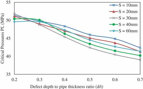
Figure 7 shows the variations of the normalized ratio of FEA results over the RSTRENG results with the defect depth to thickness ratios. Figure 7 is used to estimate the missing function in Equation (5)(5) $P_f=f\left(d/t\right)\ast \left[{\sigma }_s+68.95\ast \frac{2t}{D}\ast \left(\frac{1-0.85d/t}{1-0.85d/t\ast \frac{1}{M}}\right)\right]$(5) .

Figure 7. Relationship between the ratio of FEA over RSTRENG method and d/t

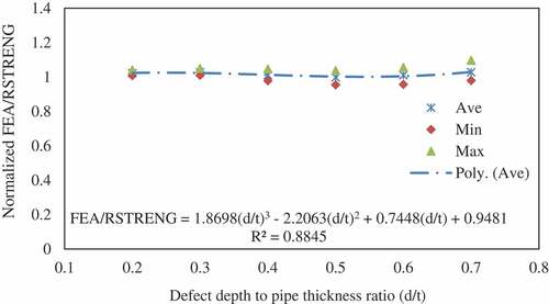
Accordingly, Equation (7)(7) $f\left(d/t\right)=\left(1.8698{(d/t)}^3-2.2063{(d/t)}^2+0.7448\left(d/t\right)+0.9481\right)$(7) is obtained by fitting the data in Figure 7 based on the mean values of the ratio of the finite element results over the RSTRENG results.

(7) $f\left(d/t\right)=\left(1.8698{(d/t)}^3-2.2063{(d/t)}^2+0.7448\left(d/t\right)+0.9481\right)$(7)

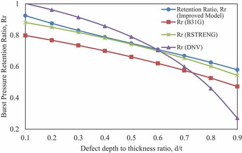
The remaining strength of the pipe was estimated in terms of the pressure retention ratio; this is the ratio of the failure pressure of the corroded pipe and the initial design pressure of the pipe. The variation between the finite element method and the RSTRENG method can be accounted for with Equation (7)(7) $f\left(d/t\right)=\left(1.8698{(d/t)}^3-2.2063{(d/t)}^2+0.7448\left(d/t\right)+0.9481\right)$(7) . The combination of the Equations (5)(5) $P_f=f\left(d/t\right)\ast \left[{\sigma }_s+68.95\ast \frac{2t}{D}\ast \left(\frac{1-0.85d/t}{1-0.85d/t\ast \frac{1}{M}}\right)\right]$(5) and (7(7) $f\left(d/t\right)=\left(1.8698{(d/t)}^3-2.2063{(d/t)}^2+0.7448\left(d/t\right)+0.9481\right)$(7) ) yields Equation (8)(8) $p_f=\left\{1.8698{\left(\frac{d}{t}\right)}^3-2.2063{\left(\frac{d}{t}\right)}^2+0.7448\left(\frac{d}{t}\right)+0.9481\right\}\left[{\sigma }_s+68.95\ast \frac{2t}{D}\ast \left(\frac{1-0.85d/t}{1-0.85d/t\ast \frac{1}{M}}\right)\right]$(8) , which better failure pressure predictions according to Figure 8. From the figure, the ASME B31G method has the fastest decline in strength, with the lowest pressure retention ratios, whereas the DNV method shows optimistic retention ratios initially but declines rather too quickly with deeper defects. However, the RSTRENG method shows more improved pressure retention ratios. The developed model, Equation (5)(5) $P_f=f\left(d/t\right)\ast \left[{\sigma }_s+68.95\ast \frac{2t}{D}\ast \left(\frac{1-0.85d/t}{1-0.85d/t\ast \frac{1}{M}}\right)\right]$(5) , on the other hand, estimates a fair retention ratio both in the cases of shallow defects and deeper defects. An important feature of the developed model is that it can be applied regardless of the distance between the defects once the distance between the defects satisfies the criterion for defects interaction under the ASME B31G code.

(8) $p_f=\left\{1.8698{\left(\frac{d}{t}\right)}^3-2.2063{\left(\frac{d}{t}\right)}^2+0.7448\left(\frac{d}{t}\right)+0.9481\right\}\left[{\sigma }_s+68.95\ast \frac{2t}{D}\ast \left(\frac{1-0.85d/t}{1-0.85d/t\ast \frac{1}{M}}\right)\right]$(8)

Figure 8. Strength estimations of the corroded pipeline using different methods

4. Conclusion

Remaining strength estimation of corroded pipelines is a major consideration in pipeline integrity management. The loss of pipe wall thickness due to corrosion inevitably leads to a reduction in the pipeline’s strength and ability to contain pressure. If corrosion defects are closely spaced, the corrosion feature may interact, resulting in failure pressure, lower than would be expected if the defects were evaluated as separate flaws. In such a situation, industry methods for remaining strength calculation have been shown to be conservative. This present work presents a new model that improves the current methodologies for estimating the remaining strength of a corroded pipeline with interacting defects, utilizing an FEA approach in combination with curve fitting. ANSYS FEA software was used to simulate selected cases of corrosion feature interaction on a pipeline section. The results obtained from the FEA were used to develop a fitting model, which was used to modify the remaining strength (RSTRENG) formula. The coupling of the FEA fitted model and the RSTRENG formula was achieved through the ratio of failure/burst pressures under the FEA and RSTRENG. The new model demonstrates the potentials of improved estimation of the remaining strength over the existing industry models for all cases of defects—shallow and deep defects. The implication is that the presented model has the potentials of reducing the conservatism inherent in the existing models for estimating the remaining strength of oil and gas pipelines.

Acknowledgments

The first author wishes to acknowledge the financial sponsorship of the Petroleum Technology Development Fund (PTDF) toward his MSc degree program at the Offshore Technology Institute, University of Port Harcourt, Nigeria.

Additional information

Funding

This work was supported by the Petroleum Technology Development Fund, Nigeria .

Notes on contributors

K.U. Amandi

K.U. Amandi He is currently studying for a Master’s degree in Pipeline Engineering at the Offshore Technology Institute, University of Port Harcourt, Nigeria. He is a Petroleum Engineering graduate from the prestigious Federal University of Technology Owerri, Nigeria. His interest is in pipeline engineering and oil and gas asset management.

E.O. Diemuodeke

O.E. Diemuodeke He obtained his PhD degree from Cranfield University, UK. He holds M.Eng and B.Eng degrees in Mechanical Engineering from the University of Port Harcourt, Nigeria. He is a fellow of the Massachusetts Institute of Technology (MIT). His research interests include renewable energy technologies and environmental sustainability and liquid loading on offshore structures.

T.A. Briggs

T.A. Briggs He received a PhD degree in Mechanical Engineering from the University of Nigeria and a Postgraduate Certificate in Advanced Studies in Academic Practice from the University of Newcastle. He is currently the Acting Director of the Offshore Technology Institute, University of Port Harcourt.

References

- Al-Owaisia, S., Becker, A. A., Sun, W., Al-Shabibi, A., Al-Maharbi, M., TasneemPervez, T., & Al-Salmi, H. (2018). An experimental investigation of the effect of defect shape and orientation on the burst pressure of pressurised pipes. Engineering Failure Analysis, 93, 200–9. doi:10.1016/j.engfailanal.2018.06.011
- Amaya-Gómez, R., Sánchez-Silva, M., Bastidas-Arteaga, E., Schoefs, F., & Muñoz, F. (2019). Reliability assessments of corroded pipelines based on internal pressure—A review. Engineering Failure Analysis, 98, 190–214. doi:10.1016/j.engfailanal.2019.01.064
- API 5L. (2004). Specification for line pipe. Washington: American Petroleum Institute.
- ASME B31G. (2012). Manual for determining the remaining strength of corroded pipelines: Supplement to ASME B31 code for pressure piping. New York: ASME Press.
- ASME B31.8. (2012). Gas Transmission and Distribution Piping Systems, ASME Press, New York.
- Bipul, C. M., & Ashutosh, S. D. (2017). Interaction of multiple corrosion defects on burst pressure of pipelines. Newfoundland and Labrador, Canada: Department of Civil Engineering, Memorial University of Newfoundland.
- Chanyalew, T. B., Mokhtar, C. I., & Karuppanan, S. (2011). Burst strength analysis of corroded pipelines using finite element method. Journal of Applied Sciences, 11(10), 1845–1850. doi:10.3923/jas.2011.1845.1850
- Dick, I. F., & Inegiyemiema, M. (2014). Predicting the structural response of a corroded pipeline using Finite Element (FE) Analysis. International Journal of Scientific & Engineering Research, 5(11), 194–207.
- DNV. (2010). Recommended practice for corroded pipelines RP-F101. Retrieved from http://www.dnv.com
- Karuppanan, S., Aminidin, A. S., & Wahab, A. A. (2012). Burst pressure estimation of corroded pipelines with interacting defects using Finite Element Analysis. Journal of Applied Sciences, Asian Network of Scientific Information, 12(24), 2626–2630.
- McAllister, E. W. (2000). Pipeline rules of the thumb handbook (2nd ed.). Houston: Gulf Publishing Company, New York.
- Mohitpour, M., Golshan, H., & Murray, A. (2000). Pipeline design & construction—A practical approach (2nd ed.). New York: ASME Press.
- Ossai, C. I. (2017). Estimation of corroded pipelines in consideration of burst pressures—A fractural mechanics approach. Infrastructure, 2(15). doi:10.3390/infrastructures2040015
- Wang, Y., Li, C., Chang, R., & Huang, H. (2016). State evaluation of a corroded pipeline. Journal of Marine Engineering & Technology, 15(2), 88–96. doi:10.1080/20464177.2016.1224615