Model of quality costs and economic benefits of a business process of manufacturing companies

Abstract

The objective of the study is to develop a mathematical model to measure the quality cost and economic benefits of the implementation of the quality improvement program within a business process of manufacturing companies. The economic benefits are obtained from saving quality costs resulting from achieving operational performance targets. The research methodology is used; firstly, the authors developed a conceptual model as a basis for a mathematical model. Secondly, they used a numerical experiment to illustrate the measurement of the effect of the change of the model parameters’ values (e.g. number of performance indicators, and level target of performance target) toward the performance target achieved, cost savings obtained, and economic benefits. If the value of the model parameters increases, then the economic benefits will increase as well, and give a shorter return period of investment. And vice versa, if the value of the model parameters decreases, then the economic benefits will decrease as well and give a longer return period of investment. The model describes the dynamics of the quality costs and economic benefits periodically obtained from a quality improvement program.

Keywords:

• quality cost
• performance target
• cost savings
• economic benefits
• payback period

PUBLIC INTEREST STATEMENT

The research in this article was conducted to investigate and offer solutions for calculating quality costs and economic benefits from implementing quality improvement programs. The companies can use this model to assist in making decisions about the optimal budget for quality improvement programs and for determining the level of target performance. This decision is needed, with the consideration that quality improvement investments must provide profits and returns in a short time. The authors got many questions from the company’s top leaders about whether an investment in quality improvement programs such as the implementation of management system standards is beneficial from a financial perspective. If it is profitable, when will it happen? This kind of questions encourages researchers to develop mathematical models related to this.

1. Introduction

The objective of a quality cost system is to measure the success of the quality improvement process and ensure that the investment in a quality improvement program is cost-effective. Top management in a manufacturing company often ask questions such as how much investment is needed for a quality improvement program and if the impact on the company performance is worth the cost spent (Øvretveit, 2000).

Bester (1999) stated that investment in a quality improvement program must be in conformity with the quality and profitability level of the company. Profitability is fulfilled by the achievement of each work unit’s quality objectives which contributes to the achievement of the company’s overall goals. Angel and Chandra (2001) propose a multi-level model that tracks the impact of quality improvement cost programs on the results of work unit performance, such as sales turnover, manufacturing and inventory cost efficiency, and failure costs. This model explores the impact of the costs of quality improvement on various prevention and appraisal activities within a business process in a manufacturing company. Furthermore, Visawan and Tannock (2004) stated that investment in quality management programs such as Kaizen (e.g. for the improvement program of design quality and the quality of the product) has an impact on selling prices in the market, as selling prices are sensitive to quality levels. This kind of cases shows that quality improvement program costs are a trade-off between costs spent and benefits obtained (Setijono & Dahlgaard, 2008).

Even though the quality improvement program is considered a determining factor for successful operational performance (Antunes, Quirós, & Justino, 2018), other research shows a negative relationship with performance (Scarpin & Brito, 2017). Negative results may be related to the costs of implementing and maintaining quality improvement programs. Because quality improvement programs require a cost, in the short term they can have an impact on increasing the operating costs, while the program has not shown a direct reduction in costs (Regina & Brito, 2018). Such conditions are a challenge for companies trying to prove that in the long run, a quality improvement program should provide an impact on financial performance (Sturm, Kaiser, & Hartmann, 2019).

The studies that integrate both the quality costs and the economic benefits through periodical quality improvement programs are still rare. Therefore, this paper develops a model of quality costs and economic benefits for the implementation of the quality improvement program considering the time dynamics.

This paper is organised as follows. First, the background chapter refers to several studies that discuss the cost of quality and its impact on the company. The second chapter discusses the results of the literature review on traditional, modern and dynamic quality cost models. The third chapter discusses the research methodology, including the development of conceptual and mathematical models for measuring quality costs and economic benefits. The fourth chapter focuses on the behaviour of the model through numerical experiments for several scenario changes in model parameters. The fifth chapter presents the research results and discussion, and the sixth chapter contains conclusions, theoretical and practical contributions, as well as the limitations of research for future research.

2. Literature study

The quality cost system is important because the total quality costs consume about 25% of the resources used by a company (Chopra & Garg, 2012; Fons, 2011; Malik, Khalid, Zulqarnain, & Iqbal, 2016). A high percentage of total quality costs indicates that an organisation should have an effective quality cost reduction program (Sturm et al., 2019).

2.1. The Preventive-Appraisal-Failure (PAF) quality cost model

The quality cost category of Preventive-Appraisal-Failure (PAF) was developed by Feigenbaum in 1956 (Schiffauerova & Thomson, 2006). The PAF model explains how the optimal quality levels can be achieved by investing on the costs of prevention and appraisal in order to reduce failure costs and to achieve a minimum total quality cost (Figure 1).

Figure 1. The traditional quality cost model

Although the PAF model is universally accepted for determining quality costs, it has some limitations, such as that the view of PAF quality costs regarding optimal quality levels does not follow the philosophy of quality improvement. This PAF model is static and so it does not take into account the dynamic aspects of time in increasing the optimal quality level (Kim & Nakhai, 2008).

The disadvantage of the static quality cost model is that it is contrary to the philosophy of zero defects in continuous quality improvement. Moreover, it does not consider the dynamic behaviour of quality levels from period to period. Through continuous quality improvement programs, prevention and appraisal costs should not need as much investment as required at the beginning of the quality improvement program. If it is assumed that cost of prevention and appraisal decreases over time, the total quality costs will decrease as the cost of product/service failure decreases as a result of the improving quality (Kerfai, Ghadhab, & Malouche, 2016). In Figure 2, the concept of quality improvement costs is referred to as the modern quality cost model (Schiffauerova & Thomson, 2006).

Figure 2. The modern quality cost model

2.2. The dynamic quality cost model

Kim and Nakhai (2008) validate the behaviour of the modern quality costs that take into account dynamics time in quality improvement programs. The preventive-appraisal costs are assumed to be the cost of improving quality IC(t) to achieve the quality level QL(t), and the costs of failure FC(t). Then, the quality improvement and failure costs are assumed to be the total quality cost TC(t) in the period t given by Equation (1)(1) $\mathrm{T}\mathrm{C}\left(\mathrm{t}\right)=\mathrm{I}\mathrm{C}\left(\mathrm{t}\right)+\mathrm{F}\mathrm{C}\left(\mathrm{t}\right)$(1) as follows.

(1) $\mathrm{T}\mathrm{C}\left(\mathrm{t}\right)=\mathrm{I}\mathrm{C}\left(\mathrm{t}\right)+\mathrm{F}\mathrm{C}\left(\mathrm{t}\right)$(1)

The quality level QL(t) depends on all the quality improvement efforts carried out in the period 1, 2, …, t or QL(t) is a function of IC(1), IC(2), … IC(t-1). The effectiveness of IC(t) on QL(t) can be different for each period IC(1), IC(2), …, IC(t-1), which is expressed as a parameter α (0 ≤α ≤1).

The level of quality QL(t) is an ascending concave function at the effectiveness of the cost of quality improvement A(t) as shown in Equation (2)(2) $\begin{array}{rl}& \mathrm{Q}\mathrm{L}\left(\mathrm{t}\right)=\mathrm{f}[\mathrm{A}\left(\mathrm{t}\right)=\mathrm{f}[\mathrm{I}\mathrm{C}\left(\mathrm{t}\right)+\alpha \mathrm{I}\mathrm{C}\left(\mathrm{t}-1\right)+{\alpha }^2\mathrm{I}\mathrm{C}\left(\mathrm{t}-2\right)+\dots +{\alpha }^{\mathrm{t}-1}\mathrm{I}\mathrm{C}\left(1\right)]\\ & =\mathrm{f}\left[{\sum }_{\mathrm{k}=0}^{\mathrm{t}-1}{\alpha }^{\mathrm{k}}\mathrm{I}\mathrm{C}\left(\mathrm{t}-\mathrm{k}\right)\right]\end{array}$(2) and Figure 3:

(2) $\begin{array}{rl}& \mathrm{Q}\mathrm{L}\left(\mathrm{t}\right)=\mathrm{f}[\mathrm{A}\left(\mathrm{t}\right)=\mathrm{f}[\mathrm{I}\mathrm{C}\left(\mathrm{t}\right)+\alpha \mathrm{I}\mathrm{C}\left(\mathrm{t}-1\right)+{\alpha }^2\mathrm{I}\mathrm{C}\left(\mathrm{t}-2\right)+\dots +{\alpha }^{\mathrm{t}-1}\mathrm{I}\mathrm{C}\left(1\right)]\\ & =\mathrm{f}\left[{\sum }_{\mathrm{k}=0}^{\mathrm{t}-1}{\alpha }^{\mathrm{k}}\mathrm{I}\mathrm{C}\left(\mathrm{t}-\mathrm{k}\right)\right]\end{array}$(2)

Based on Equation (2)(2) $\begin{array}{rl}& \mathrm{Q}\mathrm{L}\left(\mathrm{t}\right)=\mathrm{f}[\mathrm{A}\left(\mathrm{t}\right)=\mathrm{f}[\mathrm{I}\mathrm{C}\left(\mathrm{t}\right)+\alpha \mathrm{I}\mathrm{C}\left(\mathrm{t}-1\right)+{\alpha }^2\mathrm{I}\mathrm{C}\left(\mathrm{t}-2\right)+\dots +{\alpha }^{\mathrm{t}-1}\mathrm{I}\mathrm{C}\left(1\right)]\\ & =\mathrm{f}\left[{\sum }_{\mathrm{k}=0}^{\mathrm{t}-1}{\alpha }^{\mathrm{k}}\mathrm{I}\mathrm{C}\left(\mathrm{t}-\mathrm{k}\right)\right]\end{array}$(2) , the dynamic quality cost model is developed to explain the relationship between QL(t) and A(t). Based on the Pareto effect (Juran & Godfrey, 1998), increasing QL(t) dramatically is often obtained in the early stages of the quality improvement program, then in the subsequent period increasing QL(t) slows down. Thus, the quality level at a given time is a function of the level of quality in the previous period (Goswami, Kumar, & Ghadge, 2019).

Figure 3. The relationship between the quality level QL(t) and quality costs A(t)

Kim and Nakhai (2008) have explained the relationship between quality costs and quality levels well by considering time dynamics of t. Unfortunately, the model does not measure the relationship between quality costs and cost savings obtained from the achievement of the company’s operational performance targets. Operational performance covers the level of product quality, delivery on time, the quality level of raw materials, and production efficiency (International Organization for Standardization, 2013).

2.3. Quality cost model and return on investment

Pursglove and Dale (1995) stated that, although the total quality costs could not be predicted, the investment in the quality improvement process was paid off in the first year. The highest quality costs occur at the beginning of the quality improvement process and tend to decrease in every subsequent period where the quality improvement process has obtained positive results. Furthermore, Bester (1999) shows that, as a result of the quality improvement process, there is a relationship between the quality cost and the quality value. In this case, the quality value is defined as the achievement of a company’s operational performance. The company seeks to reduce the cost of the quality improvement process and increase the quality value, meaning it needs to evaluate and decide on the optimal exchange between quality value and cost quality (Sawan, Low, & Schiffauerova, 2018).

3. Research method

This research method begins with conducting a literature study related to relevant topics in order to obtain a research gap. Based on the research gap, and to supplement the research already carried out on relevant topics, the purpose of this paper is to develop conceptual models and mathematical models for measuring quality costs and the economic benefits of implementing quality improvement programs. The results of the model are verified using a numerical experiment to study model behaviour based on the model parameters and it changes. The results of the numerical experiment are used for discussion and are related to the results of previous studies. The research steps are illustrated in Figure 4 as follows.

Figure 4. Research steps

3.1. The conceptual model for the measurement of quality improvement cost and economic benefits

This model is a development of the dynamic quality cost model by Kim and Nakhai (2008), as it adds measurements of economic benefits from the investment results of the quality improvement program to achieve operational performance targets, and estimates of the investment return. The development of the conceptual model is illustrated in Figure 5.

Figure 5. The conceptual model for the cost of quality improvement and economic benefits

The conceptual model in Figure 5 shows that in period 1, the company spent the quality cost of TC(1). The quality cost is used for the implementation of the quality improvement program within a business process. According to the results of the implementation, the company is successful in achieving the performance target of PI(1). Then the company obtained cost savings of PS(1). Thus, in the subsequent period t = 2,3 …, t, TC(t) can be reduced. The proportion of reduction in quality improvement costs per period is assumed by a parameter value α (0 ≤α ≤1), thus TC(1) >TC(2) > … >TC(t). While PI(t) is increased in the subsequent period, the proportion of the increase in the performance target per period is assumed by a parameter value β (0≪ β≪1); thus PI(1)<PI(2)< … <PI(t). As an effect, the company obtained cost savings of PS(t) which increased from period to period.

3.2. The mathematical model for the measurement of quality improvement costs and economic benefits

3.2.1. The total cost of the quality improvement

The total cost of the quality improvement during the period t, TQC(t), is given by Equation (3)(3) $\mathrm{T}\mathrm{Q}\mathrm{C}\left(\mathrm{t}\right)=\mathrm{T}\mathrm{C}\left(1\right)+\alpha \mathrm{T}\mathrm{C}\left(2\right)+{\alpha }^2\mathrm{T}\mathrm{C}\left(3\right)+\dots +{\mathrm{a}}^{\mathrm{k}}\mathrm{T}\mathrm{C}(\mathrm{t})=\sum _{\mathrm{k}=0,\mathrm{t}=1}^{\mathrm{\infty }}{\alpha }^{\mathrm{k}}\mathrm{T}\mathrm{C}\left(\mathrm{t}\right)$(3) , and is an ascending convex function against the effectiveness of the quality improvement program cost.

(3) $\mathrm{T}\mathrm{Q}\mathrm{C}\left(\mathrm{t}\right)=\mathrm{T}\mathrm{C}\left(1\right)+\alpha \mathrm{T}\mathrm{C}\left(2\right)+{\alpha }^2\mathrm{T}\mathrm{C}\left(3\right)+\dots +{\mathrm{a}}^{\mathrm{k}}\mathrm{T}\mathrm{C}(\mathrm{t})=\sum _{\mathrm{k}=0,\mathrm{t}=1}^{\mathrm{\infty }}{\alpha }^{\mathrm{k}}\mathrm{T}\mathrm{C}\left(\mathrm{t}\right)$(3)

The TQC(t) is used to achieve the performance target in period t, PI(t). Thus, PI(t) is an ascending concave function against TQC(t), which shows how successful achieving the performance target is. Likewise, PI(t = f[TQC(t)]) is given by Equation (4)(4) $\mathrm{P}\mathrm{I}\left(\mathrm{t}\right)=\mathrm{f}[\mathrm{T}\mathrm{Q}\mathrm{C}\left(\mathrm{t}\right)]=\mathrm{f}[\mathrm{T}\mathrm{C}\left(1\right)+\alpha \mathrm{T}\mathrm{C}\left(2\right)+{\alpha }^2\mathrm{T}\mathrm{C}\left(3\right)+\dots +{\alpha }^{\mathrm{k}}\mathrm{T}\mathrm{C}\left(\mathrm{t}\right)]=\mathrm{f}\left[\sum _{\mathrm{k}=0,\mathrm{t}=1}^{\mathrm{\infty }}{\alpha }^{\mathrm{k}}\mathrm{T}\mathrm{C}\left(\mathrm{t}\right)\right]$(4) and illustrated in Figure 6.

(4) $\mathrm{P}\mathrm{I}\left(\mathrm{t}\right)=\mathrm{f}[\mathrm{T}\mathrm{Q}\mathrm{C}\left(\mathrm{t}\right)]=\mathrm{f}[\mathrm{T}\mathrm{C}\left(1\right)+\alpha \mathrm{T}\mathrm{C}\left(2\right)+{\alpha }^2\mathrm{T}\mathrm{C}\left(3\right)+\dots +{\alpha }^{\mathrm{k}}\mathrm{T}\mathrm{C}\left(\mathrm{t}\right)]=\mathrm{f}\left[\sum _{\mathrm{k}=0,\mathrm{t}=1}^{\mathrm{\infty }}{\alpha }^{\mathrm{k}}\mathrm{T}\mathrm{C}\left(\mathrm{t}\right)\right]$(4)

Figure 6. The relationship between the level of the target performance, PI(t) and the total quality cost, TQC(t)

The level of the performance target achieved in period t is an ascending concave function against the total quality improvement cost, PI(t) = f[TQC(t)] and is a function as given in Equation (5)(5) $\mathrm{f}\left(\mathrm{x}\right)=\frac{{\mathrm{x}}^{1/\left({\prod }_{\mathrm{i}=1}^{\mathrm{n}}{\beta }_{\mathrm{i}}\right)}}{\mathrm{m}+{\mathrm{x}}^{1/\left({\prod }_{\mathrm{i}=1}^{\mathrm{n}}{\beta }_{\mathrm{i}}\right)}}$(5) .

(5) $\mathrm{f}\left(\mathrm{x}\right)=\frac{{\mathrm{x}}^{1/\left({\prod }_{\mathrm{i}=1}^{\mathrm{n}}{\beta }_{\mathrm{i}}\right)}}{\mathrm{m}+{\mathrm{x}}^{1/\left({\prod }_{\mathrm{i}=1}^{\mathrm{n}}{\beta }_{\mathrm{i}}\right)}}$(5)

Where m > 0, and β_i is the specific parameter of the company. Notation β_i shows the target level of the performance indicator to i, where i = 1,2, …, n (n = number of performance indicators).

The function of achieving the performance indicator target, f(x) should fulfil the following properties:

1. f(x) is a concave function increased against the total quality improvement cost, x. Besides, according to the Pareto principle, the increase in the achievement of the performance target in subsequent periods tends to slow down along with the total quality improvement cost spent;

2. Achievement of performance targets is given as a value of f (x), where 0 ≤f(x)≤1; and lim x→∞ f(x) = 1, f(0) = 0.

3.2.2. The total cost savings

The total cost saving obtained in period t, PS(t) is an ascending convex function against the achievement of the target performance in period t, PS(t) = g[PI(t)] (Figure 7). The curvature of this convex curve is influenced by the target level of the performance indicator, β. The higher the parameter value β (0≪ β≪1), the more cost savings will be obtained. Thus,

(6) $\text{PS}\left(\text{t}\right)\text{=}\text{g}[\text{PI}\left(\text{t}\right)]\text{=}\text{g}[\text{PI}\left(\text{1}\right)\text{+}\beta \text{PI}\left(\text{2}\right)\text{+}{\beta }^{\text{2}}\text{PI}\left(\text{3}\right)\text{+}\dots \text{+}{\beta }^{\text{k}}\text{PIt=g}\left[{\displaystyle \sum _{\text{k}=0,\text{t}=1}^{\infty }{\beta }^{\text{k}}}\text{PI}\left(\text{t}\right)\right]$(6)

Figure 7. The relationship between cost savings, PS(t) and the target performance achieved, PI(t)

The cost saving obtained is an ascending convex function against the target performance achieved, PS(t) = f[PI(t)] and the function is as given in Equation (7)(7) $\mathrm{g}\left(\mathrm{y}\right)={\mathrm{y}}^{1/\left({\sum }_{\mathrm{i}=1}^{\mathrm{n}}{\beta }^{\mathrm{i}-1}\ast \mathrm{c}\right)}$(7) .

(7) $\mathrm{g}\left(\mathrm{y}\right)={\mathrm{y}}^{1/\left({\sum }_{\mathrm{i}=1}^{\mathrm{n}}{\beta }^{\mathrm{i}-1}\ast \mathrm{c}\right)}$(7)

Where c (0 <c ≤1) shows the weight of the contribution from the performance indicator in a business function to the total performance indicator contribution from all business functions, and β_i shows the target level of the performance indicator to i, where i = 1,2, …, n (n = number of performance indicators). The parameter value c affects the magnitude of the contribution of performance indicators to cost savings. For example, the performance indicator in the business function of the production process makes a more significant contribution to the total contribution than the performance indicator in the inbound logistics business function (Sohal & Prajogo, 2012). Therefore, the performance indicators within the production process contribute more to the savings costs obtained.

The function g(y) should fulfil the following properties:

1. g(y) is a convex function increased with the achievement of the target performance, y. According to the Pareto principle, the increase in cost savings slows down along with the increased achievement of the target performance level; and

2. The cost savings obtained are given as a value of g (y), where 0 ≤g(y) ≤1; where lim y→∞ g(y) = 1, and g(0) = 0.

3.2.3. The economic benefits

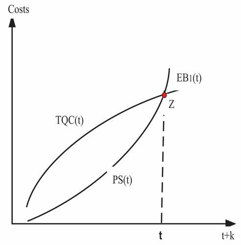
The economic benefits (EB) from the results of a quality improvement program are the total cost savings minus the total quality improvement cost in period t as given by Equation (9). If the value of EB(t) is positive (EB > 0), then the company acquires benefits from a quality improvement program. And vice versa, if the value of EB(t) is negative (EB < 0), then the company loses.

(8) $\mathrm{E}\mathrm{B}\left(\mathrm{t}\right)=\mathrm{P}\mathrm{S}\left(\mathrm{t}\right)-\mathrm{T}\mathrm{Q}\mathrm{C}\left(\mathrm{t}\right)$(8)

Figure 8 shows a trade-off between the total quality cost, TQC(t) and the total cost savings, PS(t). In period t, the company reaches a break-even point (Z) between the total cost of quality improvement and the cost savings (TQC(t) = PS(t)), and in period t +k the company starts to get positive results (profits).

Figure 8. The economic benefits of the quality improvement program

4. A numerical experiment and the result

As a numerical experiment, the values of the quality cost model parameters were taken from Kim and Nakhai (2008), namely the cost of quality improvement program in period 1 is 5% or TC(1) = 0.05 and the effectiveness of the quality improvement costs is 95% (α = 0.95). While the target level of performance indicator in period 1 is 95% (β = 0.95), and the specific parameter of the company is m = 0.01. Meanwhile, the weight of the contribution of the process business’ performance indicator to the total contribution of the company’s performance indicators is 5% (c = 0.05),

In addition, the calculation is carried out for a) total cost of quality improvement, TQC(t), which uses Equation (3)(3) $\mathrm{T}\mathrm{Q}\mathrm{C}\left(\mathrm{t}\right)=\mathrm{T}\mathrm{C}\left(1\right)+\alpha \mathrm{T}\mathrm{C}\left(2\right)+{\alpha }^2\mathrm{T}\mathrm{C}\left(3\right)+\dots +{\mathrm{a}}^{\mathrm{k}}\mathrm{T}\mathrm{C}(\mathrm{t})=\sum _{\mathrm{k}=0,\mathrm{t}=1}^{\mathrm{\infty }}{\alpha }^{\mathrm{k}}\mathrm{T}\mathrm{C}\left(\mathrm{t}\right)$(3) ; b) achievement of the performance target, PI_i(t) which is a function of TQC(t) and uses Equations (4)(4) $\mathrm{P}\mathrm{I}\left(\mathrm{t}\right)=\mathrm{f}[\mathrm{T}\mathrm{Q}\mathrm{C}\left(\mathrm{t}\right)]=\mathrm{f}[\mathrm{T}\mathrm{C}\left(1\right)+\alpha \mathrm{T}\mathrm{C}\left(2\right)+{\alpha }^2\mathrm{T}\mathrm{C}\left(3\right)+\dots +{\alpha }^{\mathrm{k}}\mathrm{T}\mathrm{C}\left(\mathrm{t}\right)]=\mathrm{f}\left[\sum _{\mathrm{k}=0,\mathrm{t}=1}^{\mathrm{\infty }}{\alpha }^{\mathrm{k}}\mathrm{T}\mathrm{C}\left(\mathrm{t}\right)\right]$(4) and (5(5) $\mathrm{f}\left(\mathrm{x}\right)=\frac{{\mathrm{x}}^{1/\left({\prod }_{\mathrm{i}=1}^{\mathrm{n}}{\beta }_{\mathrm{i}}\right)}}{\mathrm{m}+{\mathrm{x}}^{1/\left({\prod }_{\mathrm{i}=1}^{\mathrm{n}}{\beta }_{\mathrm{i}}\right)}}$(5) ); c) total cost savings obtained, PS_i(t) which is a function of PI_i(t) and uses Equations (6)(6) $\text{PS}\left(\text{t}\right)\text{=}\text{g}[\text{PI}\left(\text{t}\right)]\text{=}\text{g}[\text{PI}\left(\text{1}\right)\text{+}\beta \text{PI}\left(\text{2}\right)\text{+}{\beta }^{\text{2}}\text{PI}\left(\text{3}\right)\text{+}\dots \text{+}{\beta }^{\text{k}}\text{PIt=g}\left[{\displaystyle \sum _{\text{k}=0,\text{t}=1}^{\infty }{\beta }^{\text{k}}}\text{PI}\left(\text{t}\right)\right]$(6) and (7(7) $\mathrm{g}\left(\mathrm{y}\right)={\mathrm{y}}^{1/\left({\sum }_{\mathrm{i}=1}^{\mathrm{n}}{\beta }^{\mathrm{i}-1}\ast \mathrm{c}\right)}$(7) ); and d) economic benefits, EB_i(t), which uses Equation (8)(8) $\mathrm{E}\mathrm{B}\left(\mathrm{t}\right)=\mathrm{P}\mathrm{S}\left(\mathrm{t}\right)-\mathrm{T}\mathrm{Q}\mathrm{C}\left(\mathrm{t}\right)$(8) . An example of the calculation in Period 2 for 1 performance indicator is done using a Microsoft Excel spreadsheet, and the result is as follow.

• Using Equation (3)(3) $\mathrm{T}\mathrm{Q}\mathrm{C}\left(\mathrm{t}\right)=\mathrm{T}\mathrm{C}\left(1\right)+\alpha \mathrm{T}\mathrm{C}\left(2\right)+{\alpha }^2\mathrm{T}\mathrm{C}\left(3\right)+\dots +{\mathrm{a}}^{\mathrm{k}}\mathrm{T}\mathrm{C}(\mathrm{t})=\sum _{\mathrm{k}=0,\mathrm{t}=1}^{\mathrm{\infty }}{\alpha }^{\mathrm{k}}\mathrm{T}\mathrm{C}\left(\mathrm{t}\right)$(3) ,                • Using Equations (4)(4) $\mathrm{P}\mathrm{I}\left(\mathrm{t}\right)=\mathrm{f}[\mathrm{T}\mathrm{Q}\mathrm{C}\left(\mathrm{t}\right)]=\mathrm{f}[\mathrm{T}\mathrm{C}\left(1\right)+\alpha \mathrm{T}\mathrm{C}\left(2\right)+{\alpha }^2\mathrm{T}\mathrm{C}\left(3\right)+\dots +{\alpha }^{\mathrm{k}}\mathrm{T}\mathrm{C}\left(\mathrm{t}\right)]=\mathrm{f}\left[\sum _{\mathrm{k}=0,\mathrm{t}=1}^{\mathrm{\infty }}{\alpha }^{\mathrm{k}}\mathrm{T}\mathrm{C}\left(\mathrm{t}\right)\right]$(4) and (5(5) $\mathrm{f}\left(\mathrm{x}\right)=\frac{{\mathrm{x}}^{1/\left({\prod }_{\mathrm{i}=1}^{\mathrm{n}}{\beta }_{\mathrm{i}}\right)}}{\mathrm{m}+{\mathrm{x}}^{1/\left({\prod }_{\mathrm{i}=1}^{\mathrm{n}}{\beta }_{\mathrm{i}}\right)}}$(5) ),

  TQC(2) = TC(1)+0.95TC(1) = 0.050 + 0.048 = 0.098     PI1(2) = $\mathrm{f}\left(0.098\right)=\frac{{0.098}^{(1/0.95)}}{0.01+{0.098}^{(1/0.95)}}$ = 0.896

• Using Equations (6)(6) $\text{PS}\left(\text{t}\right)\text{=}\text{g}[\text{PI}\left(\text{t}\right)]\text{=}\text{g}[\text{PI}\left(\text{1}\right)\text{+}\beta \text{PI}\left(\text{2}\right)\text{+}{\beta }^{\text{2}}\text{PI}\left(\text{3}\right)\text{+}\dots \text{+}{\beta }^{\text{k}}\text{PIt=g}\left[{\displaystyle \sum _{\text{k}=0,\text{t}=1}^{\infty }{\beta }^{\text{k}}}\text{PI}\left(\text{t}\right)\right]$(6) and (7(7) $\mathrm{g}\left(\mathrm{y}\right)={\mathrm{y}}^{1/\left({\sum }_{\mathrm{i}=1}^{\mathrm{n}}{\beta }^{\mathrm{i}-1}\ast \mathrm{c}\right)}$(7) ),            • Using Equation (8)(8) $\mathrm{E}\mathrm{B}\left(\mathrm{t}\right)=\mathrm{P}\mathrm{S}\left(\mathrm{t}\right)-\mathrm{T}\mathrm{Q}\mathrm{C}\left(\mathrm{t}\right)$(8) ,

  PS1(2) = $\mathrm{g}\left(0.896\right)={0.896}^{1/\left(1\ast 0.05\right)}$ = 0.111       EB1(2) = PS(2)-TQC(2) = 0.013

This means that the total cost of quality improvement programs in period 2 for 1 performance indicator, TQC (2) is 0.098 or 9.8%. For this total cost, the company’s achievement the performance target, PI1(2) of 0.896 or 89.6%. In addition, from reaching the target performance, the company obtains cost savings, PS1(2) is 0.111 or 11.1%. Thus, in period 2 the company has obtained economic benefits (profit), EB1(2) of 0.013 or 1.3%. Furthermore, the results of the numerical experiment for the 18 periods for a performance indicator i, where i = 1, 2, 3, and 4 are shown in Table 1. The distribution of data from numerical experiments is given in Figure 9.

Table 1. The results of the numerical experiment for TC(1) = 0.05, α = 0.95, β = 0.95, m = 0.01, and c = 0.05 for 18 periods and four performance indicators

Period	TC(t)	TQC(t)	1 performance indicator, β = 0.95			2 performance indicators, β = 0.95
			PI1(t)	PS1(t)	EB1(t)	PI1(t)	PS1(t)	EB1(t)
1	0.05	0.05	0.81	0.015	−0.035	0.783	0.082	0.032
2	0.048	0.098	0.896	0.111	0.014	0.883	0.281	0.183
3	0.045	0.143	0.928	0.224	0.081	0.92	0.427	0.284
4	0.043	0.185	0.944	0.318	0.133	0.939	0.526	0.34
5	0.041	0.226	0.954	0.393	0.167	0.951	0.595	0.369
6	0.039	0.265	0.961	0.452	0.187	0.958	0.646	0.381
7	0.037	0.302	0.966	0.5	0.198	0.964	0.684	0.382
8	0.035	0.337	0.969	0.538	0.202	0.968	0.714	0.377
9	0.033	0.37	0.972	0.57	0.2	0.971	0.738	0.368
10	0.032	0.401	0.975	0.597	0.195	0.973	0.757	0.356
11	0.03	0.431	0.976	0.619	0.188	0.975	0.773	0.342
12	0.028	0.46	0.978	0.639	0.179	0.977	0.787	0.327
13	0.027	0.487	0.979	0.656	0.169	0.978	0.798	0.312
14	0.026	0.512	0.98	0.67	0.158	0.979	0.808	0.296
15	0.024	0.537	0.981	0.683	0.146	0.98	0.817	0.28
16	0.023	0.56	0.982	0.694	0.134	0.981	0.824	0.264
17	0.022	0.582	0.983	0.704	0.122	0.982	0.831	0.249
18	0.021	0.603	0.983	0.713	0.11	0.983	0.837	0.234
Period	TC(t)	TQC(t)	3 performance indicators, β = 0.95			4 performance indicators, β = 0.95
			PI1(t)	PS1(t)	EB1(t)	PI1(t)	PS1(t)	EB1(t)
1	0.05	0.05	0.752	0.136	0.086	0.717	0.166	0.116
2	0.048	0.098	0.869	0.373	0.275	0.852	0.421	0.323
3	0.045	0.143	0.912	0.523	0.38	0.902	0.572	0.429
4	0.043	0.185	0.933	0.617	0.431	0.927	0.663	0.478
5	0.041	0.226	0.946	0.68	0.454	0.942	0.723	0.497
6	0.039	0.265	0.955	0.724	0.459	0.951	0.764	0.5
7	0.037	0.302	0.961	0.757	0.456	0.958	0.795	0.493
8	0.035	0.337	0.966	0.782	0.446	0.963	0.818	0.481
9	0.033	0.37	0.969	0.802	0.433	0.967	0.835	0.466
10	0.032	0.401	0.972	0.818	0.417	0.97	0.85	0.448
11	0.03	0.431	0.974	0.831	0.4	0.973	0.861	0.43
12	0.028	0.46	0.976	0.842	0.383	0.975	0.871	0.411
13	0.027	0.487	0.977	0.852	0.365	0.976	0.879	0.392
14	0.026	0.512	0.979	0.86	0.347	0.978	0.886	0.374
15	0.024	0.537	0.98	0.866	0.33	0.979	0.892	0.355
16	0.023	0.56	0.981	0.872	0.312	0.98	0.897	0.337
17	0.022	0.582	0.982	0.878	0.296	0.981	0.901	0.32
18	0.021	0.603	0.982	0.882	0.279	0.982	0.905	0.303

Figure 9. The relationship between TQC(t) and PS_i(t) for each number of indicators (i = 1,2,3,4) for β = 0.95

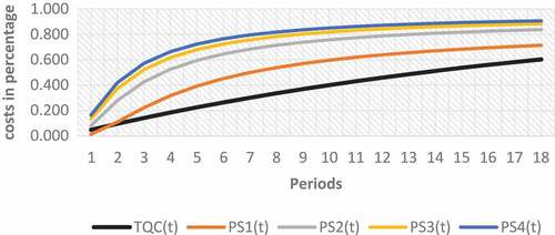
In period 1, the target performance achieved, PI_i(1) for the number of performance indicators (i = 1, 2, 3, 4) in a business process is 81.0, 78.3, 75.2, and 71.7% respectively. The level of target performances achieved shows that with the same total cost of quality improvement, it is more difficult for companies to achieve target performances when there are more performance indicators. The results are lower than the target performances with fewer performance indicators.

The cost savings obtained are 0.15, 8.2, 13.6, and 16.6% respectively. Contrary to the results of reaching the target performance, the company that determines only one performance indicator in a business process, had relatively small cost savings. However, if the company determines more than 1 performance indicator, the cost savings are relatively large, even though the level of target performance achieved is lower. This is because of the contribution of the number of performance indicators in case of more than one indicator.

Furthermore, the economic benefits obtained are −3.5, 3.2, 8.6, and 11.6% respectively. In period t = 1, when the number of performance indicators is 1 (one), the company loses because the total cost of quality is greater than the cost savings obtained. However, for more than one performance indicator, the company makes a profit, because the cost savings obtained are greater than the total quality costs.

Figure 9 shows that the curvature of the cost-saving function depends on the number of performance indicators. If the number of performance indicators increases, then the function of the cost savings becomes increasingly convex. Thus, the cost savings will increase, and the economic benefits increase too. However, from Figure 9, it is recommended to set a maximum of 3 performance indicators in business processes, because if the number of performance indicators is higher, the increase in cost savings is not significant.

4.1. Changes of parameters model

If the target level of the performance set in a business process is 80% (β = 0.80), then the numerical experiment for four performance indicators and for the 18 periods shows different results (Table 2). A thorough distribution of data from numerical experiments is given in Figure 10.

Table 2. The results of the numerical experiment for TC(1) = 0.05, α = 0.95, β = 0.80, m = 0.01, and c = 0.05 for 18 periods and four performance indicators

Period	TC(t)	TQC(t)	1 performance indicator, β = 0.80			2 performance indicators, β = 0.80
			PI1(t)	PS1(t)	EB1(t)	PI2(t)	PS2(t)	EB2(t)
1	0.05	0.05	0.703	0.001	−0.049	0.481	0	−0.05
2	0.048	0.098	0.845	0.034	−0.063	0.725	0.028	−0.07
3	0.045	0.143	0.898	0.115	−0.027	0.827	0.121	−0.022
4	0.043	0.185	0.924	0.206	0.021	0.878	0.235	0.05
5	0.041	0.226	0.94	0.289	0.062	0.907	0.34	0.114
6	0.039	0.265	0.95	0.359	0.094	0.926	0.427	0.162
7	0.037	0.302	0.957	0.417	0.115	0.939	0.496	0.195
8	0.035	0.337	0.962	0.465	0.129	0.948	0.553	0.216
9	0.033	0.37	0.966	0.506	0.136	0.955	0.598	0.228
10	0.032	0.401	0.97	0.54	0.138	0.96	0.635	0.234
11	0.03	0.431	0.972	0.569	0.138	0.964	0.666	0.235
12	0.028	0.46	0.974	0.594	0.134	0.967	0.692	0.232
13	0.027	0.487	0.976	0.615	0.128	0.97	0.714	0.227
14	0.026	0.512	0.977	0.634	0.121	0.972	0.732	0.22
15	0.024	0.537	0.979	0.65	0.113	0.974	0.748	0.212
16	0.023	0.56	0.98	0.664	0.105	0.976	0.762	0.202
17	0.022	0.582	0.981	0.677	0.095	0.977	0.774	0.192
18	0.021	0.603	0.982	0.689	0.086	0.978	0.785	0.182
Period	TC(t)	TQC(t)	3 performance indicators, β = 0.80			4 performance indicators, β = 0.80
			PI3(t)	PS3(t)	EB3(t)	PI4(t)	PS4(t)	EB4(t)
1	0.05	0.05	0.223	0	−0.05	0.062	0	−0.05
2	0.048	0.098	0.515	0.004	−0.093	0.254	0	−0.097
3	0.045	0.143	0.69	0.048	−0.095	0.463	0.005	−0.137
4	0.043	0.185	0.788	0.142	−0.043	0.621	0.039	−0.146
5	0.041	0.226	0.846	0.254	0.027	0.726	0.115	−0.112
6	0.039	0.265	0.882	0.357	0.092	0.796	0.213	−0.052
7	0.037	0.302	0.906	0.445	0.143	0.843	0.314	0.012
8	0.035	0.337	0.923	0.517	0.18	0.875	0.405	0.068
9	0.033	0.37	0.935	0.575	0.205	0.898	0.483	0.113
10	0.032	0.401	0.944	0.623	0.221	0.915	0.548	0.146
11	0.03	0.431	0.951	0.662	0.23	0.928	0.601	0.17
12	0.028	0.46	0.956	0.694	0.234	0.937	0.646	0.186
13	0.027	0.487	0.961	0.72	0.234	0.945	0.682	0.196
14	0.026	0.512	0.964	0.743	0.231	0.951	0.713	0.201
15	0.024	0.537	0.967	0.762	0.225	0.956	0.739	0.202
16	0.023	0.56	0.97	0.778	0.218	0.96	0.761	0.201
17	0.022	0.582	0.972	0.792	0.211	0.964	0.779	0.197
18	0.021	0.603	0.974	0.805	0.202	0.967	0.795	0.192

Figure 10. The relationship between TQC(t) and PS_i(t) for each number of indicators (i = 1,2,3,4) for β = 0.80

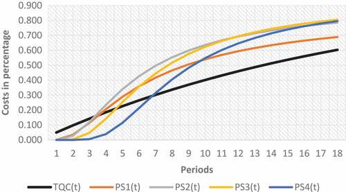
In Table 2 and Figure 10, in period 1, the target performance achieved, PI_i(1) for the number of performance indicators i (i = 1, 2, 3, 4) in a business process is 70.3, 48.1, 22.3, and 6.2% respectively. Thus, the cost savings obtained, PS_i(1) are 0.01, 0.00, 0.00, and 0.00% respectively. This result shows that with a target level of performance indicator of 80% (β = 0.80), in period 1, the company loses. The company obtains economic benefits, EB_i(t) for each number of performance indicators i (I = 1,2,3, and 4) are in periods 4, 4, 5 and 7 respectively.

5. Discussion

For β = 0.95, the greater the number of performance indicators, the greater the cost savings and the faster the return period on the quality investments. In addition, companies that set a high target level of performance will have the larger cost savings. Thus, the bigger the number of indicators and the higher the target level of performance, the bigger the economic benefits and the shorter the return period on the quality investments.

Conversely, if the target level of performance is low, for example, β = 0.80, the greater the number of performance indicators, the smaller the cost savings and the longer the return period on the quality investment. In Table 2 and Figure 10, for β = 0.80, companies must be careful when deciding the number of performance indicators. Because the results of the model behaviour show that a large number of indicators does not guarantee greater cost savings. In this numerical experiment, three is the recommended number of performance indicators, because after period 12, the company obtains a higher cost savings compared to the number of performance indicators 1, 2 or 4.

The mathematical model developed serves to integrate the dynamic quality cost model (Kim & Nakhai, 2008) and the concept of getting a return from a static quality cost investment (Bester, 1999), and to answer the conceptual model of investment for a quality improvement program (Øvretveit, 2000), through measuring the cost of improving quality, achievement of target performance, and the economic benefits obtained from cost savings on a business process from period to period. This model can be used to answer questions from Regina and Brito (2018) which state that quality improvement programs often do not show a direct reduction in costs. In the model developed, the cost of quality improvement programs can be directly reduced through cost savings obtained from the achievement of target performances. In addition, this model answers questions from a number of companies that in the long run, quality improvement programs affect the company’s financial performance (Sturm et al., 2019).

6. Conclusion

The economic benefits of implementing a quality improvement program are influenced by the amount of investment in quality improvement programs, the number of performance indicators and target levels, and the weight of the contributions from performance indicators in a business process to the total contribution of all business processes in manufacturing companies. For higher levels of target performance, the number of indicators increases, and the cost savings are greater. However, for lower levels of target performance, an increasing number of indicators does not guarantee that the greater savings will be obtained. For this reason, the company must be right when deciding the target level of the performance indicator.

6.1. Theoretical contributions

This model is the development of a dynamic quality cost model (Kim & Nakhai, 2008), where the model only discusses the relationship between the cost of quality improvement and the quality level. But this research model adds measurements of economic benefits from the investment results of quality improvement costs to achieve operational target performance and estimates of the investment return period of quality improvement programs from period to period. In addition, in contrast to research with relevant topics, the majority of which uses an empirical research approach, this study uses a mathematical model approach along with model parameters that allow companies to directly estimate the relationship between quality costs spent, economic benefits obtained, and the period of return on investment.

6.2. Managerial implications

Top management can use this model to assist in making decisions about the optimal budget for quality improvement programs and for determining the level of target performance in a business process. This decision is needed, with the consideration that quality improvement investments must provide profits and returns in a short time. The company should determine the value of the parameters such as target level and the number of performance indicators. Thus, the company can see the extent to which the quality improvement program is feasible if measured from the quality costs incurred and the economic impacts obtained.

6.3. Limitations of the research and future research directions

Because this study is only limited to the discussion of one business process in a manufacturing company, the next study needs to consider how the performance of a business process affects the performance of subsequent business processes. For example, the performance in the inbound logistics process affects the performance in the production process, while the performance in the production process affects the performance of the outbound logistics process, etc. Thus, future research is the development of a model which considers the interdependent relationship among business processes within a manufacturing company.

Additional information

Funding

The authors received no direct funding for this research.

Notes on contributors

Muhammad Rosiawan

Muhammad Rosiawan was granted his Master’s Degree in Industrial Engineering from Institut Teknologi Bandung, Indonesia. He actively assists several organisations in implementing management system standards. His research interests include cost of quality and integrated management system.

Moses Laksono Singgih

Moses Laksono Singgih is a professor of productivity and quality at the Department of Industrial Engineering at Institut Teknologi Sepuluh Nopember. He has a Master’s Degree in Industrial Engineering, from the Institut Teknologi Bandung, Indonesia and a Ph.D in Industrial Economics, University of Queensland, Australia. His current research interest is in productivity and quality in manufacturing systems.

Erwin Widodo

Erwin Widodo was granted his Master’s Degree from Ritsumeikan University of Kyoto and his Doctoral Degree from Hiroshima University both in Japan. His expertise is in multi-player decision-making in industry especially by using game theory. He actively joins several international associations related to his field, i.e. IAEng, IEOM, as well as a board member in several international journals such as IJISE, Cogent Engineering, etc.

References

- Angel, L. C., & Chandra, M. J. (2001). Performance implications of investments in continuous quality improvement. International Journal of Operations & Production Management, 21(1951), 108–15. doi:10.1108/01443570110358486
- Antunes, M. G., Quirós, J. T., & Justino, M. R. (2018). Total quality management and quality certification : Effects in organisational performance. International Journal Services and Operations Management, 29(4), 439–461. doi:10.1504/IJSOM.2018.090452
- Bester, Y. (1999). Qualimetrics and qualieconomics. The TQM Magazine, 11(6), 425–436. doi:10.1108/09544789910287755
- Chopra, A., & Garg, D. (2012). Introducing models for implementing cost of quality system. The TQM Journal, 24(6), 498–504. doi:10.1108/17542731211270061
- Fons, L. A. S. (2011). Measuring economic effects of quality management systems. The TQM Journal, 23(4), 458–474. doi:10.1108/17542731111139527
- Goswami, M., Kumar, G., & Ghadge, A. (2019). An integrated Bayesian – Markovian framework for ascertaining cost of executing quality improvement programs in manufacturing industry. International Journal of Quality & Reliability Management, 36, 1229–1242. doi:10.1108/IJQRM-10-2018-0280
- International Organization for Standardization. (2013). Economic benefits of standards- ISO methodology 2.0. Geneva: ISO Central Secretariat.
- Juran, J. M., & Godfrey, A. B. (1998). Juran’s quality control handbook. New York, NY: McGrawHill.
- Kerfai, N., Ghadhab, B. B., & Malouche, D. (2016). Performance measurement and quality costing in Tunisian manufacturing companies. The TQM Journal, 28(4), 588–596. doi:10.1108/TQM-10-2013-0119
- Kim, S., & Nakhai, B. (2008). The dynamics of quality costs in continuous improvement. International Journal of Quality & Reliability Management, 25(8), 842–859. doi:10.1108/02656710810898649
- Malik, T. M., Khalid, R., Zulqarnain, A., & Iqbal, S. A. (2016). Cost of quality : Findings of a wood products ’ manufacturer. The TQM Journal, 28(1), 2–20. doi:10.1108/TQM-01-2014-0014
- Øvretveit, J. (2000). The economics of quality – A practical approach. International Journal of Health Care Quality Assurance, 13(5), 200–207. doi:10.1108/09526860010372803
- Pursglove, A. B., & Dale, B. G. (1995). Developing a quality costing system: Key features and outcomes. Omega, 23(5), 567–575. doi:10.1016/0305-0483(95)00027-L
- Regina, M., & Brito, L. A. L. (2018). Operational capabilities in an emerging country : Quality and the cost trade-off effect. International Journal of Quality & Reliability Management, 35(8), 1617–1638. doi:10.1108/IJQRM-04-2017-0061
- Sawan, R., Low, J. F., & Schiffauerova, A. (2018). Quality cost of material procurement in construction projects. Engineering, Construction and Architectural Management, 25(8), 974–988. doi:10.1108/ECAM-04-2017-0068
- Scarpin, M. R. S., & Brito, L. A. L. (2017). Operational capabilities in an emerging country: Quality and the cost trade-off effect. International Journal of Quality & Reliability Management, 17, 460–471.
- Schiffauerova, A., & Thomson, V. (2006). A review of research on cost of quality models and best practices. International Journal of Quality & Reliability Management, 23(6), 647–669. doi:10.1108/02656710610672470
- Setijono, D., & Dahlgaard, J. J. (2008). The value of quality improvements. International Journal of Quality & Reliability Management, 25(3), 292–312. Retrieved from http://www.emeraldinsight.com/doi/10.1108/02656710810854296
- Sohal, A., & Prajogo, D. (2012). ISO 9001: The drivers for installation and maintenance, Departmet of Management, Monash University and JAS-ANZ.
- Sturm, S., Kaiser, G., & Hartmann, E. (2019). Long-run dynamics between cost of quality and quality performance dynamics. International Journal of Quality & Reliability Management. doi:10.1108/IJQRM-05-2018-0118
- Visawan, D., & Tannock, J. (2004). Simulation of the economics of quality improvement in manufacturing: A case study from the Thai automotive industry. International Journal of Quality and Reliability Management, 21(6), 638–654. doi:10.1108/02656710410542043