Pseudo-spectral optimal control of stochastic processes using Fokker Planck equation

Abstract

Motivated by the successful implementation of Pseudo-spectral (PS) methods in optimal control problems (OCP), a new technique is introduced to control the probability density function (PDF) of the state of the 1-D system described by a stochastic differential equation (SDE). In this paper, the Fokker Planck equation (FPE) is used to model the time evolution of the PDF of the stochastic process. Using FPE instead of SDE, changes the problem of stochastic optimal control to a deterministic one. FPE is a parabolic PDE. Solving an OCP with PDE constraint is computationally a difficult task. We use two strategies to efficiently solve this OCP problem: firstly, we use PS methods in order to transform the OCP to a non-linear programming (NLP) with fewer discretization points but higher order of accuracy, and secondly, we utilize Genetic algorithm (GA) to solve this large-scale NLP in a more efficient approach than gradient-based optimization methods. The simulation results based on Monte-Carlo simulations prove the performance of the proposed method.

Keywords:

• Pseudo-spectral optimal control
• Fokker Planck equation
• stochastic process
• genetic algorithm
• Legendre pseudo-spectral method

PUBLIC INTEREST STATEMENT

Fokker Planck equation describes the time evolution of the trajectories of the stochastic differential equation. The FPE optimal control is an alternative approach to stochastic optimal control of the SDEs. Unlike, optimal control of the SDEs, FPE optimal control is a deterministic approach to solve a stochastic process. In this paper, the FPE optimal control is considered and instead of controlling the trajectories of the stochastic system, the probability density function of this trajectories have been controlled. The paper proposed a pseudo-spectral discretization strategy in combination with genetic algorithm to reduce the computational complexity of the FPE optimal control.

1. Introduction

Stochastic optimal control is one of the main subfields of control theory. It is introduced due to considering more realistic models where many systems in different branches of science are subjected to randomness. It is the subject of study in traffic control (Zhong, Sumalee, Pan, & Lam, 2014), airspace industry (Okamoto & Tsuchiya, 2015), cancer chemotherapy (Coldman & Murray, 2000), cyber security systems in computer science (Shang, 2013, 2012), etc. When the system randomness is bounded and the bounds are known, the problem of finding a suitable control action can be dealt with robust control approaches (Doyle, Francis, & Tannenbaum, 2013; Wu & Lee, 2003; Zhou & Doyle, 1998). While the bounds of uncertainty are unknown and the probability distribution of the randomness is available, the stochastic framework should be carried out in optimal control (Åström, 2012; Herzallah, 2018; Sell, Weinberger, & Fleming, 1988; Touzi, 2012). There is a vast amount of literature on stochastic optimal control of linear systems with additive noise where the certainty equivalence property leads to the separation principle in stochastic control (Bar-Shalom & Tse, 1974; Mohammadkhani, Bayat, & Jalali, 2017). Under certain conditions, separation principle asserts that finding a control action for a stochastic system can be restated as designing a stable observer and a stable controller. In the other words, a stochastic problem can be recast as two deterministic problems. Linear quadratic Gaussian control (LQG) is one of the most prominent stochastic control methods. It is simply the combination of Kalman filter as an observer and a linear quadratic controller.

In spite of much research on the subject of separation principle for nonlinear systems (Atassi & Khalil, 1999; Khalil, 2008), no general separation principle exists for nonlinear systems. Rich theoretical foundations in the literature regarding the deterministic optimal control encourage control engineers to convert stochastic optimal control into a corresponding deterministic one. One approach to remodel a stochastic process into a deterministic counterpart is using Fokker Planck equation (FPE). FPE is a parabolic PDE that models the time evolution of probability density function (PDF) of a stochastic process. PDF of the states of a stochastic process fully characterize the statistical behaviour of the states. Under this scheme, the control function is sought such that the PDF of the states reaches to a desired PDF in time.

Several studies have been published on stochastic optimal control using FPE in the literature. In Annunziato and Borzì (2010), the FPE framework for optimal control of the 1-D stochastic process was presented. Finite difference method is utilized for discretization of the OCP. In Annunziato and Borzì (2013), the authors argued the problem of stochastic optimal control of multidimensional systems and an efficient computational method based on Chang-Cooper scheme was proposed. In Fleig, Grüne, Pesch, and Altmüller (2014), some theoretical results regarding the existence and uniqueness of the solution of FPE were proved. Also, the existence and uniqueness of the solution of stochastic optimal control using FPE have been investigated; the numerical solution was based on finite difference method. In Annunziato and Borzì (2010, 2013) and Fleig et al. (2014), the control function is only the function of time, but in Fleig and Guglielmi, it is assumed to be state dependent as well as time dependent. In Buehler, Paulson, and Mesbah (2016), a stability constraint was integrated into the FP optimal control in order to guarantee the system stabilization in probability (Battilotti & De Santis, 2003). All the aforementioned papers implement receding horizon control strategy known as model predictive control (MPC) (Camacho & Bordons, 2012; Wang, 2009). To the best of our knowledge, the focus of the literature was not on the numerical discretization of Fokker Planck optimal control.

The main contribution of this work is on the discretization of the FPE optimal control problem (OCP) using Pseudo-spectral (PS method). PS optimal control is a fast computational method for solving general OCPs. It uses the foundations of PS theory to solve an OCP. The main reason that PS method is suitably fit to the OCPs is: (1) Efficient approximation method for integration in the cost function, solving ODE that governs the dynamic of the system and discretization of the state-space constraint (Fahroo & Ross, 2008; Gong et al., 2007; Gong, Kang, & Ross, 2006). (2) There is sufficient theoretical support for convergence and consistency of PS method for optimal control based on covector mapping principle (Gong, Ross, Kang, & Fahroo, 2008; Ross, 2005), also PS method is known to be one of the top three numerical solutions of PDEs (Trefethen, 2000). In this paper, instead of approximating ODE that describes the time evolution of the state of the system in a formal PS optimal control framework, we approximate the Fokker Planck PDE which is the dynamical constraint of the stochastic system.

It would be worth mentioning that not only many theoretical OCP have been solved by PS optimal control, it is also widely applied in practice. It has been successfully implemented in different NASA flight systems (Ross & Karpenko, 2012) and industrial and military applications (Gong et al., 2007). In this research, we utilize the Legendre PS method (Elnagar, Kazemi, & Razzaghi, 1995) based on Legendre-Gauss-Lobatto (LGL) points which is proven to be the most appropriate PS method for solving the finite time OCP with boundary conditions (Fahroo & Ross, 2008). Discretization of FP optimal control yields a large-scale non-linear programming (NLP) which is a hard computational problem. A new intuitive efficient technique based on Genetic algorithm (GA) is adapted to reduce the computational complexity of the NLP.

The paper is structured as follows: Section 2 gives a brief review of FPE optimal control with necessary assumptions and the main OCP is determined. PS method fundamentals are described in details in Section 3. In Section 4, the Methodology of FPE discretization and the proposed method is presented base on GA. Section 5 gives the numerical results of implementing the proposed method on three benchmark stochastic processes, and finally in Section 6, conclusions are provided and future works are described.

2. Fokker planck optimal control

A typical stochastic differential equation (SDE) is as follows:

(1) $d{X}_t=b(X_t,u_t,t)dt+\sigma (X_t,t)d{W}_{t}t\in [t_0,T]$(1)

(2) $X_t(t=t_0)=X_0$(2)

Where, $X_t\in \mathrm{\Omega }\subset R^n$ solves the stochastic differential Equation (1)(1) $d{X}_t=b(X_t,u_t,t)dt+\sigma (X_t,t)d{W}_{t}t\in [t_0,T]$(1) provided:

(3) $X_t=X_0+\underset{t_0}{\overset{T}{\int }}b(X_t,u_t,t)dt+\underset{t_0}{\overset{T}{\int }}\sigma (X_t,t)dw$(3)

$X_0$ is the initial condition, $W_t\in R^r$ is the Weiner process, $r$ is the dimension of Weiner process, $b(X_t,t):R^n\times [t_0,T]\to R^n$ is a vector valued drift function and $\sigma (X_t,t):R^n\times [t_0,T]\to R^{n\times r}$ is a vector valued diffusion function. $u_t\in R^m$ is the control function, which is considered to be the function of time. The first Integral in (3) is Lebesgue integral and the second one is Ito Integral. Here we consider 1-D SDE where $n=m=r=1$.

To ensure the existence and uniqueness of the solution of Equation (1)(1) $d{X}_t=b(X_t,u_t,t)dt+\sigma (X_t,t)d{W}_{t}t\in [t_0,T]$(1) , the following assumptions must be satisfied. For each realization of $W_t$, $\mathrm{\exists }C>0$, $\mathrm{\forall }x,y\in R$, $t\in [t_0,T]$, $u\in R$

$\left|b(x,u,t)-b(y,u,t)\left|+\right|\sigma (x,t)-\sigma (y,t)\left|\le C\right|x-y\right|$

$\left|b(x,u,t){|}^2+\right|\sigma (x,t){|}^2\le C^2(1+|x{|}^2)$

Definition 2.1 (The FPE initial boundary problem) the corresponding Fokker Planck equation of (1) is defined as follows:

(4) $\frac{\mathrm{\partial }p(x,t)}{\mathrm{\partial }t}+\sum _{i=1}^n\frac{\mathrm{\partial }(b(x,u,t)p(x,t))}{\mathrm{\partial }{x}_i}-\frac{1}{2}\sum _{i=1}^n\sum _{j=1}^n\frac{{\mathrm{\partial }}^2(a_{ij}(x,t)p(x,t))}{\mathrm{\partial }{x}_i\mathrm{\partial }{x}_j}=0inQ$(4)

with initial and boundary conditions:

$p(x,0)=\rho (x)in\mathrm{\Omega }$

$p(x,t)=0in\sum$

Where $p(x,t)$ is the PDF of $X_t$ at time $t$, $b$ and $\sigma$ are the drift and diffusion functions corresponding to SDE (1). $Q=\mathrm{\Omega }\times (t_0,T)$, $\sum =\mathrm{\partial }\mathrm{\Omega }\times (t_0,T)$ and $\rho (x=X_0)$ is the initial distribution. Also $a=\sigma (x,t)\sigma (x,t{)}^T$ is a positive symmetric matrix called diffusion matrix.

Remark 1 Equation (4)(4) $\frac{\mathrm{\partial }p(x,t)}{\mathrm{\partial }t}+\sum _{i=1}^n\frac{\mathrm{\partial }(b(x,u,t)p(x,t))}{\mathrm{\partial }{x}_i}-\frac{1}{2}\sum _{i=1}^n\sum _{j=1}^n\frac{{\mathrm{\partial }}^2(a_{ij}(x,t)p(x,t))}{\mathrm{\partial }{x}_i\mathrm{\partial }{x}_j}=0inQ$(4) is a parabolic type PDE with initial and boundary condition. According to the probability axioms, the solution of PDE (4) should satisfy:

$p(x,t)\ge 0,(x,t)\in Q$

$\underset{\mathrm{\Omega }}{\int }p(x,t)dx=1,t\ge t_0$

The existence and uniqueness of the Fokker Planck initial boundary value problem are addressed in (Fleig et al., 2014).

Definition 2.2 (The FPE optimal control problem): The Fokker Planck equation optimal control problem is a dynamic optimization problem with PDE constraint, it could be formulated as:

Problem 1

$u^{\ast }(p(x,t))={arg}_{u}minJ=\underset{0}{\overset{T}{\int }}(\frac{\alpha }{2}\mathrm{\Delta }(p(x,t),P_{ref}(x,t))+\frac{\beta }{2}||u(t)|{|}_R^2)dt$

Subject to:

(5a) $FPE(4)inQ$(5a)

(5b) $p(x,0)=\rho (x)in\mathrm{\Omega }$(5b)

(5c) $p(x,t)=0in\mathrm{\Sigma }$(5c)

(5d) $u\in U_{ad}=\{u\in U|u_a\le u\le u_b\}\subset U:=R$(5d)

where $\mathrm{\Delta }(t)$ is a measure of similarity between $p(x,t)$, PDF of state, and $P_{ref}(x,t)$, the desired PDF. $\alpha ,\beta \in R>0$ are the performance trade-off constants. $u_a,u_b\in R$ are upper and lower bounds on the admissible set of control $U_{ad}$. (5a) shows that the Problem. 1 is a dynamic optimization problem that should satisfy the FPE (4) as its constraint.

Remark 2: The FPE equation is a second-order PDE, and for solutions we need boundary condition. Condition (5c) is called absorbing boundary condition (Mohammadi, 2015). For absorbing boundary condition, the boundaries are chosen such that the probability on the boundaries is zero. The condition (5d) is control constraint condition. Due to physical restrictions in practical systems, the control signals cannot be arbitrary large, so imposing control constraint is necessary for most of OCP.

The existence of the solution of such OCP with PDE constraints is discussed in (Hinze, Pinnau, Ulbrich, & Ulbrich, 2008).

3. PS fundamentals

PS approximation was initially developed to solve PDEs. In this method, continuous functions are approximated in a finite set of nodes called collocation nodes. These nodes are selected in a way that guarantees the high accuracy of approximation. The main exclusivity of PS method is in the smart selection of collocation nodes. Assume that a real value function $f(t)$ is going to be approximated in $[-1,1]$ with some interpolants. The simplest but worst choices of nodes are equal distance nodes. But if a special set of nodes such as roots of derivative of Legendre polynomial known as LGL is chosen, the higher accuracy with fewer nodes can be achieved. The following inequality shows the impressive convergence speed of PS method.

(6) $||f(t)-I_{N}f(t)|{|}_{L^2}\le \frac{C}{N^m}$(6)

Where $I_{N}f(t)$ is the polynomial interpolation of $f(t)$. $C$ is a constant. $N$ is the number of collocation points and $m$ is the order of differentiability of $f(t)$. If $f(t)\in C^{\mathrm{\infty }}$ $(m=\mathrm{\infty })$ the polynomial converges at a spectral rate.

There are two types of numerical methods to solve an OCP, direct and indirect methods. Indirect methods use the calculus of variation such as Pontryagin minimum principle. These methods are usually hard to solve numerically. Direct methods are known as discretize-then-optimize methods. They are not based on the calculus of variation. In direct methods, the state and control function are approximated by function approximation such as polynomial approximation.

When an OCP is solved by direct methods, it is highly desirable to use few number of discretization point. A typical OCP consists of three mathematical equations: (1) Integration in the cost function; (2) Differential equation governing the system state evolution; and (3) Algebraic equations appear as the constraints. PS method is suitable for approximation of all three objects. The OCP studied in this paper is different from a typical PS OCP because instead of an ODE constraint, the PDE constraint is utilized which is the FPE.

There are a lot of theoretical proofs regarding the convergence, consistency and optimality of the solution of PS optimal control. It should be noted that these results are true for systems that are described by the ODE. In this paper, no theoretical proof has been proposed for FP PS optimal control but numerical results prove the validity of the method.

In this paper, we chose the Gauss PS method with Lagrange interpolant. Since the OCP is finite time, the LGL nodes are used for discretization. Here the necessary foundations of PS method for optimal control are discussed . We show that in PS framework, the differentiations in dynamic constraint of OCP, as well as integration in the cost function can be converted to algebraic equations.

3.1. Domain transformation

For Gauss-PS method when solving a finite-horizon OCP, the computational framework is $[-1,1]$, so variables such as time and states, should be scaled as follows:

Domain transformation of time

$t\in [t_0,t_f]$

(7) $\tau =Z(t)=\frac{2}{t_f-t_0}t-\frac{t_f+t_0}{t_f-t_0}$(7)

Domain transformation of $x$

$x\in [x_0,x_f]$

(8) $X=Y(x)=\frac{2}{x_f-x_0}x-\frac{x_f+x_0}{x_f-x_0}$(8)

3.2. Interpolation

Given $\tau =[{\tau }_0,{\tau }_1,...,{\tau }_{N_t}]$ and $X=[X_0,X_1,...,X_{N_x}]$, set of distinct points in $[-1,1]$, a standard Lagrange interpolant for control function $u(t)$ and $x(t)$ can be written as:

(9a) $u(t)\approx u^{N_t}(t)=\sum _{i=1}^{N_t}u({\tau }_i)L_i^{N_t}(\tau )$(9a)

(9b) $x(t)\approx x^{N_X}(t)=\sum _{i=1}^{N_X}x(X_i)L_i^x(X)$(9b)

Where $u^{N_t}(t)$ and $x^{N_X}(t)$ are a unique polynomial of degree $N_t$ and $N_X$, respectively. $L_i^{N_{\hspace{0.17em}}}(\tau )$ is the N-th order Lagrange polynomial

(10) $L_i^N(\tau )=\prod _{\genfrac{}{}{0ex}{}{j=1}{j\ne i}}^N\frac{\tau -{\tau }_j}{{\tau }_i-{\tau }_j}$(10)

that satisfies the Kronecker property $L_i^N({\tau }_j)={\delta }_{ij}$. This implies that $u({\tau }_j)=u^{N_t}({\tau }_j)$ and $x(X_j)=x^{N_X}(X_j)$. Also, the interpolation for PDF of state $p(x,t)$ can be written as second Lagrange form interpolant as follows:

(11) $p(x,t)\approx p^{N_t\times N_x}(x,t)=\sum _{i=0}^{N_x}\sum _{j=0}^{N_t}p(X_i,{\tau }_j)L_i(X)L_j(\tau )$(11)

3.3. Differentiation

3.3.1. Differentiation of one variable function

As discussed before, any function can be approximated using Lagrange interpolant on the set of LGL nodes $\tau =[{\tau }_0,{\tau }_1,...,{\tau }_{N_t}]$:

$f(x)\approx f^N(x)=\sum _{i=1}^{N}f({\tau }_i)L_i^N(x)$

Also it can be expressed as matrix multiplication form

(12) $f^N(x)=L^N(x)F$(12)

where $L^N(x)=[{L_1}^N(x),{L_2}^N(x),...,{L_N}^N(x)]$ and $F=[f({\tau }_0),f({\tau }_1),...,f({\tau }_N)]$ is the value of $f(x)$ at LGL nodes.

The first derivative of $f(x)$ using interpolation can be written as

(13) $\dot{f}(x)\approx {\dot{f}}^N(x)=\sum _{i=1}^{N}f({\tau }_i){\dot{L}}_i^N(x)$(13)

where ${\dot{L}}_i^N(\tau )$ can be expressed as

(14) ${\dot{L}}_i^N(\tau )=\sum _{j=1}^N{\dot{L}}_i^N({\tau }_j)L_j^N(\tau )$(14)

By these two equations, the derivative of $f(x)$ at the LGL nodes ${\tau }_k\in [-1,1]$ can be approximated as

(15) $\dot{f}({\tau }_k)\approx {\dot{f}}^N({\tau }_k)=\sum _{j=1}^N{D}_{kj}f({\tau }_j)$(15)

where in the matrix form it can be rewritten at all LGL node as

(16) $\dot{f}(x)\approx {\dot{f}}^N(x)=D_{N+1}F$(16)

where $D_{N+1}$ is a $(N+1)\times (N+1)$ matrix defined by:

(17) $D_{N+1}=[D_{kj}]=\left\{\begin{array}{c}\frac{L({\tau }_k)}{L({\tau }_j)}\frac{1}{{\tau }_k-{\tau }_j}if,k\ne j\\ \frac{N(N+1)}{4}if,k=j=0\\ \frac{-N(N+1)}{4}if,k=j=N\\ 0otherwise\end{array}\right.$(17)

It is obvious that the approximation of $\dot{f}(x)$ only depends on $f(x)$ . For unscaled nodes i.e. ${\tau }_k\in [a,b]$ the derivative of $f(x)$ at the LGL nodes is as follows:

(18) $f^n(x)\approx f^{n^{N_{\hspace{0.17em}}}}(x)={\left(\frac{2}{b-a}\right)}^n(D_{N+1}{)}^{n}F$(18)

where $n$ is the order of derivation.

3.3.2. Differentiation of two variable function

For $g(x,y):[a,b]\times [c,d]\to R$ with arbitrary number of LGL nodes, $N$ and $M$ in each direction the Lagrange form of interpolant is

$g(x,y)\approx g^{N\times M}(x,y)=\sum _{i=0}^N\sum _{j=0}^{M}g({\tau }_i,X_j)L_i(\tau )L_j(X)$

It can be written in matrix form as

(19) $g^{N\times M}(x,y)=(L^N(x)\otimes L^M(y))G$(19)

where $\otimes$ represents the tensor product and

$G=[g({\tau }_0,X_0),...,g({\tau }_0,X_M)|g({\tau }_1,X_0),...,g({\tau }_1,X_M)|...|g({\tau }_N,X_0),...,g({\tau }_N,X_M){]}^T$ is a $(N+1)\times (M+1)$ matrix representing values of $g(x,y)$ at the LGL nodes.

For the approximation of partial differential of $g(x,y)$with respect to $x$ we have:

(20) $\frac{d}{dx}g(x,y)=(\frac{d}{dx}{L}^N(x)\otimes L^M(y))G=\frac{2}{b-a}(L^N(x)D_{N+1}\otimes L^M(y))G$(20)

At the exact LGL nodes, the derivative can be written as

(21) $\frac{d}{dx}g(x,y)=\frac{2}{b-a}(D_{N+1}\otimes I_{M+1})G$(21)

where $I_{M+1}$ is an $(M+1)\times (M+1)$ identity matrix. The higher order derivative at the LGL nodes can be written as

(22) $\frac{d^n}{d{x}^n}g(x,y)=(\frac{2}{b-a}{)}^n((D_{N+1}{)}^n\otimes I_{M+1})G$(22)

The approximation of partial differential of $g(x,y)$ with respect to $y$ at the LGL nodes can be deduced as

(23) $\frac{d}{dy}g(x,y)=\frac{2}{d-c}(I_{N+1}\otimes D_{M+1})G$(23)

And for higher derivative order we have

(24) $\frac{d^n}{d{y}^n}g(x,y)={\left(\frac{2}{d-c}\right)}^n(I_{N+1}\otimes (D_{M+1}{)}^n)G$(24)

Similar operations on tensor have been also used in other works, e.g. (Shang, 2014).

3.4. Integration

In PS method, the integration is approximated by Gaussian quadrature rule.

(25) $\underset{-1}{\overset{1}{\int }}f(x)dx=\sum _{i=1}^N{w}_{i}f(x_i)$(25)

where in Gauss PS method $x_i,i=1,...,N$ are LGL nodes and $w_i,i=1,...,N$ are predetermined quadrature weights correspond to LGL nodes. For arbitrary domain of integration over $[a,b]$, the Gauss quadrature rule can be rewritten as

(26) $\underset{a}{\overset{b}{\int }}f(x)dx=\frac{b-a}{2}\sum _{i=1}^N{w}_{i}f(\frac{b-a}{2}x+\frac{a+b}{2})$(26)

4. PS discretization of FP optimal control

Using fundamentals that have been discussed in Section 3, all mathematical objects that form an OCP, i.e. Integration, PDE and constraints can be discretized using PS method. By defining the meshes in each direction, ${\pi }^{N_t}=\{{\tau }_0,{\tau }_1,...,{\tau }_{N_t}\}$ and ${\pi }^{N_X}=\{X_0,X_1,...,X_{N_X}\}$, we have a grid of meshes, ${\pi }^{N_t\times N_X}$, which the values of $p(x,t)$ and $u(t)$ should be defined in. Problem. 1 convert to Problem. 2 that can be solved by NLP tool.

Problem. 2

$min{J}^{N_t}(u^{N_t}(\tau ),x^{N_X}(X))=\frac{b-a}{2}\sum _{i=1}^{N_t}{w}_i\left(\frac{\alpha }{2}\mathrm{\Delta }({\tau }_i)+\frac{B}{2}||u({\tau }_i)|{|}_R^2\right)$

Subject to:

(27a) $\mathrm{\Psi }(u^{N_t}(\tau ),D_{N_t+1},D_{N_X+1})\times P=0$(27a)

(27b) $P{|}_{X_i,{\tau }_{0:N}=0}=\rho (X_i)$(27b)

(27c) $P{|}_{X_0=x_a,X_{N_X}=x_b,{\tau }_i}=0$(27c)

(27d) $u\in U_{ad}=\{u\in U|u_a\le u\le u_b\}\subset U:=R$(27d)

The solution of Problem. 2 is the vector

$Y_{[(N_t+1)(N_X+1)+(N_t+1)]\times 1}=[P_{1\times (N_t+1)(N_X+1)}^T;U_{1\times (N_t+1)}^T]$ i.e. the value of $p(x,t)$ and $u(t)$ at the LGL nodes. $P=[p(X_0,{\tau }_0),...,p(X_{N_X},{\tau }_0)|p(X_0,{\tau }_1),...,p(X_{N_X},{\tau }_1)|...|,p(X_0,{\tau }_N),...,p(X_{N_X},{\tau }_N){]}^T,U_{\hspace{0.17em}}=[u({\tau }_0),u({\tau }_1),...,u({\tau }_{N_t})]$

By calculation of these vectors and putting them in (15) and (3.2), the continuous functions $p(x,t)$ and $u(t)$ can be calculated.

The summation in Problem. 2 is the discretized counterpart of integral in Problem. 1. In this paper, for similarity of $p(x,t)$ to $P_{ref}(x,t)$ the correlation coefficient criteria is adopted as follows:

(28) $Delta({\tau }_i)={\sqrt{1-corrcoef(p(x,{\tau }_i),p_{ref}(x,{\tau }_i))}}_{\hspace{0.17em}}i=1,2,..,N_t$(28)

(27a) is the discretized model of FP equation which is a nonlinear algebraic equation.

Since $u^{N_t}(\tau )$ appears as the coefficients of $P$, the optimization is NLP. (27b) is the initial condition i.e. the initial PDF of the states . $P{|}_{X_i:X_{N_X},{\tau }_0=0}$ is defined as

(29) $P{|}_{X_i:X_{N_X},{\tau }_0=0}=[p(X_0,{\tau }_0),p(X_1,{\tau }_0),...,p(X_{N_X},{\tau }_0)]=[\rho (X_0),p(X_1),\cdots ,p(X_{N_X})]$(29)

Also in (27c), the zero boundary condition, $P{|}_{X_0=x_a,X_{N_X}=x_b,{\tau }_0:{\tau }_{N_t}}$ is defined as

(30) $P{|}_{X_0=x_a,X_{N_X}=x_b,{\tau }_0:{\tau }_{N_t}}=[p(X_0,{\tau }_0),p(X_0,{\tau }_1),...,p(X_0,{\tau }_{N_t})]=[p(X_{N_X},{\tau }_0),p(X_{N_X},{\tau }_1),\cdots ,p(X_{N_X},{\tau }_{N_t})]=[0,0,\cdots ,0]$(30)

The most challenging part of this optimization is converting the FPE to an algebraic equation i.e. finding $[\mathrm{\Psi }{]}_{(N_t+1)(N_X+1)\times (N_t+1)(N_X+1)}$ matrix . The procedure will be completely explained by different examples.

Problem. 2 is a large-scale nonlinear programming. The number of the unknowns is $N=(N_t+1)(N_X+1)+(N_t+1)$. In a typical problem, the number of meshes should be chosen as $N_t>10$ and $N_X>90$ which makes $N_t>{10}^3$. This large-scale optimization is computationally cumbersome to solve. In order to solve this problem, we intuitively reformulate Problem. 2 into a new algorithm and reduce the number of unknowns to just $N=N_t+1$ and uses genetic algorithm to find the optimal solution.

4.1. Genetic algorithm for PS-FP optimal control

In this section, we will not discuss the complete procedure of GA algorithm. It is assumed that the reader has basic knowledge about GA. For further information on GA see Whitley (1994).

The key steps of the GA-PS-FP optimal control algorithm are as follows:

1. Determine the Maximum iteration, population, percentage of mutation, crossover and other initial parameters of GA.

2. Consider $U_{\hspace{0.17em}}=[u({\tau }_0),u({\tau }_1),...,u({\tau }_{N_t})]$, control action at the LGL nodes, as individuals in GA.

3. Integrate (27a, 27b, 27c) into one linear algebraic equation $AP=B$ (FPE with initial and boundary value) with predefined values of $u^{N_t}({\tau }_i)$ as individuals. $A$ and $B$ are known Matrix and vector which are explained in the Appendix A.

4. Solve the integrated linear algebraic equation $P=A^{-1}B$

5. Calculate the fitness function of GA according to

   $J=\frac{b-a}{2}\sum _{i=1}^{N_t}{w}_i(\frac{\alpha }{2}\mathrm{\Delta }({\tau }_i)+\frac{B}{2}||u({\tau }_i)|{|}_R^2)$ Where $\mathrm{\Delta }({\tau }_i)$is defined in (28)

6. Iterate the GA until some convergence criteria have been satisfied.

Problem. 2 can be reformulated into Problem. 3 as follows:

Problem. 3

(31a) $min{J}^{N_t}(u^{N_t}(\tau ))=\frac{b-a}{2}\sum _{i=1}^{N_t}{w}_i\left(\frac{\alpha }{2}\mathrm{\Delta }({\tau }_i)+\frac{B}{2}||u({\tau }_i)|{|}_R^2\right)$(31a)

Subject to

(31b) $u\in U_{ad}=\{u\in U|u_a\le u\le u_b\}\subset U:=R$(31b)

Where $\mathrm{\Delta }({\tau }_i)=A^{-1}B-P_{ref}$ and

$P_{ref}=[p_{ref}(X_0,{\tau }_0),\cdots ,p_{ref}(X_{N_X},{\tau }_0)|p_{ref}(X_0,{\tau }_1),\cdots ,p_{ref}(X_{N_X},{\tau }_1)|\cdots |p_{ref}(X_0,{\tau }_N),\cdots ,p_{ref}(X_{N_X},{\tau }_N){]}^T$

The main advantage of this reformulation of optimization is reducing the number of unknowns to $N=N_t+1$. Also no NLP should be implemented to find the solution, instead for fitness evaluation a matrix inversion of size $(N_t+1)(N_X+1)$ must be solved.

Figure 1. Ornstein-Uhlenbleck process. (a) Desired PDF (Red) and Controlled PDF (Blue). (b) Control function Lagrange interpolation

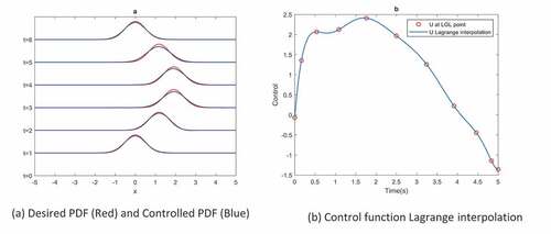
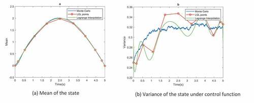
Figure 2. Ornstein-Uhlenbleck process. (a) Mean of the state. (b) Variance of the state under control function

5. Simulation results

In this section, two stochastic processes are simulated. The proposed algorithm is implemented to find the best control action. Finding the matrix $\mathrm{\Psi }$, which might be the most confusing part of the algorithm, is discussed in detail in each example. The interpolated control function is implemented to the SDEs and the Monte-Carlo runs extract the statistical characteristics of states by directly simulation of SDEs using Euler–Maruyama method (Higham, 2001). The Monte-Carlo simulation of SDEs, as well as distance between desired PDF and the PDF of the states, prove the validity of the proposed method.

Figure 3. Ornstein-Uhlenbleck process. Time evolution of probability density function of state under control function

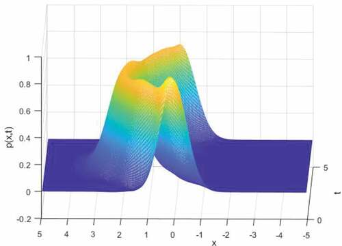
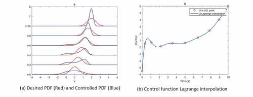
Figure 4. Typical nonlinear system

5.1. Ornstein-Uhlenbleck (OU) process

OU Process models the velocity of a massive Brownian particle under influence of friction. It is defined by

(32) $d{X}_t=(-r{X}_t+U)dt+\sigma d{W}_t$(32)

where $X$ is the velocity of the particle and $U$ is the momentum due to an external force which is the control action. The simulation parameters are determined in Table 1.

Table 1. Parameters of the simulated stochastic processes

Parameters	OU process	The typical nonlinear system
$t\in \left[t_0,t_f\right]$	$t_0=0,t_f=5$	$t_0=0,t_f=10$
$X\in \mathrm{\Omega }\in [X_0,X_f]$	$X_0=-5,X_f=5$	$X_0=-5,X_f=5$
$r$	1	1
$\sigma$	0.8	1
$P_{ref}\left(x,y\right)$	$\frac{\mathrm{e}\mathrm{x}\mathrm{p}\left(-\frac{{\left[x-2sin\left(\frac{\pi t}{5}\right)\right]}^2}{2{\left(0.5\right)}^2}\right)}{\sqrt{2\pi {\left(0.5\right)}^2}}$	$\frac{\mathrm{e}\mathrm{x}\mathrm{p}\left(-\frac{{\left[x-t/5\right]}^2}{2{\left(0.5\right)}^2}\right)}{\sqrt{2\pi {\left(0.5\right)}^2}}$
$\rho \left(x\right)$	$\frac{1}{\sqrt{2\pi {\left(0.5\right)}^2}}\mathrm{e}\mathrm{x}\mathrm{p}\left(-\frac{x^2}{2{\left(0.5\right)}^2}\right)$	$\frac{1}{\sqrt{2\pi {\left(1\right)}^2}}\mathrm{e}\mathrm{x}\mathrm{p}\left(-\frac{x^2}{2{\left(1\right)}^2}\right)$
$U_{ad}\in \left[u_a,u_b\right]$	$u_a=-4,u_b=4$	$u_a=-6,u_b=6$
$N_t$	10	10
$N_X$	100	100

By some simplifications, the corresponding FPE (40) can be written as:

(33) ${\mathrm{\partial }}_{t}p(x,t)-rp(x,t)-r{X}_t{\mathrm{\partial }}_{x}p(x,t)+U(t){\mathrm{\partial }}_{x}p(x,t)-\frac{1}{2}{\sigma }^2{\mathrm{\partial }}_{xx}p(x,t)=0$(33)

Figure 5. Typical nonlinear system

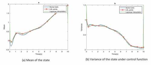
Figure 6. Typical nonlinear system. Time evolution of probability density function of state under control function

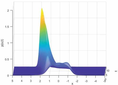
Figure 7. Typical nonlinear system with two stable equilibrium points with initial condition $\mathit{p}(x,t)=N(0,1)\mathbf{a}\mathbf{n}\mathbf{d}r=1;$

${\pi }^{N_t}=\{{\tau }_0,{\tau }_1,...,{\tau }_{N_t}\}\in [0,5]$ is chosen as the LGL nodes at time direction and ${\pi }^{N_X}=\{X_0,X_1,...,X_{N_X}\}\in [-5,5]$ as the LGL nodes at $x$ direction. The tensor product form of (33) using PS discretization at the LGL collocation points is as follows:

(34) $\begin{array}{rl}& \mathrm{\Psi }(u^{N_t}(\tau ),x^{N_X}(X),D_{N_t+1},D_{N_X+1})\times P=[\left(\frac{2}{t_f-t_e}{D}_{N_t+1}\otimes [I{]}_{(N_X+1)\times (N_X+1)}\right)\\ & -r[I{]}_{(N_t+1)\times (N_X+1)}-rdiag([\chi ])([I{]}_{(N_t+1)\times (N_t+1)}\otimes \frac{2}{x_f-x_0}{D}_{(N_X+1)})\\ & +diag([U])([I{]}_{(N_t+1)\times (N_t+1)}\otimes \frac{2}{x_f-x_0}{D}_{(N_X+1)})\\ & -\frac{1}{2}{\sigma }^2([I{]}_{(N_t+1)\times (N_t+1)}\otimes {\left(\frac{2}{x_f-x_0}\right)}^2(D_{(N_X+1)}{)}^2)]P=0\end{array}$(34)

Where $[\chi ]$and $[U]$ are $(N_t+1)(N_X+1)$ size vectors defines by

$[\chi ]=[X_0,\cdots ,X_{N_X}|X_0,\cdots ,X_{N_X}|\cdots |X_0,\cdots ,X_{N_X}{]}^T$

$[U]=[u({\tau }_0),\cdots ,u({\tau }_0)|\cdots |u({\tau }_{N_t}),\cdots ,u({\tau }_{N_t}){]}^T$

In $[\chi ]$, the vector $[X_0,...,X_{N_X}]$ repeats $N_t+1$ times. In $[U]$, the value of control action in each LGL node repeats $N_X+1$ times.

Figure 1 shows the distance between desired state PDF and the state PDF under control function and demonstrates the control function at the LGL nodes, also the interpolated control function is calculated by (10). Due to the linearity of the OU process, when the initial distribution is Gaussian, the PDF of the states are always Gaussian. So in order to test the optimal control function, it is implemented on OU and by Monte-Carlo simulations of the SDE in each time step, mean and variance at each time step is calculated. Euler–Maruyama Method is used to solve SDE in each Monte-Carlo run. Figure 2 compares the mean and variance of the states, obtained by MC simulations and FP equation. LGL points in Figure 2 represent the discretization points in time. Lagrange interpolation of this points is also demonstrated. It can be seen that the mean and variance obtained by FPE is consistent with MC simulation results. Figure 3 demonstrates the Barycentric Lagrange interpolation (Berrut & Trefethen, 2004) of $p(x,t)$ based on LGL nodes, it has been calculated at $120\times 120$ data points.

5.2. Typical nonlinear system with two stable equilibrium point

System (32) was a linear system, here we apply our method to a nonlinear system described as follows:

(35) $d{X}_t=(U+r{X}_t-{X_t}^3)dt+(\sigma X_t)d{W}_t$(35)

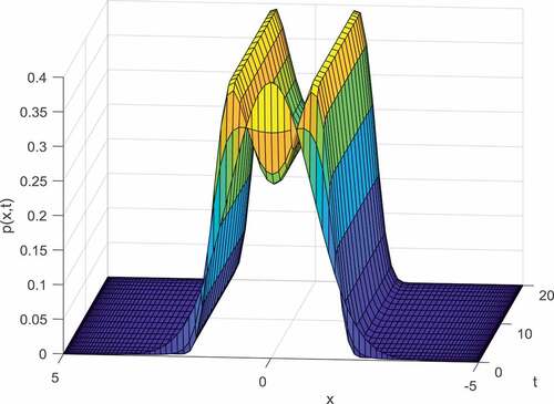
This system has 3 equilibrium points, one saddle point on $X_t=0$ and two stable points on $X_t=\pm \sqrt{r}$. As it is shown in Figure 7, the PDF of the states of autonomous system (35) with $U=0$, evolves in a bimodal Gaussian shape due to the existence of two stable Equilibrium points. The simulation parameter is summarized in Table 1.

The corresponding FPE of (35) is

(36) $\begin{array}{rl}& {\mathrm{\partial }}_{t}p(x,t)+(r-3{X_t}^2)p(x,t)+(r{X}_t-{X_t}^3+U(t)){\mathrm{\partial }}_{x}p(x,t)\\ & -\frac{1}{2}{\sigma }^2[2p(x,t)+4X_t{\mathrm{\partial }}_{x}p(x,t)+X_t^2{\mathrm{\partial }}_{xx}p(x,t)]=0\end{array}$(36)

Appendix B shows how to transform (36) to tensor product form. Figures 4 and 5 show that for nonlinear system, the proposed method succeeded to find optimal control functions and the FPE solution is consistent with MC simulations. Figure 6 demonstrates the transient PDF of the typical nonlinear system.

6. Conclusion

In this paper, a PS optimal control framework for the stochastic processes is presented. The stochastic optimal control is transformed to OCP by implementing FPE, then discretized in few collocation points by Gauss Legendre spectral discretization Method. In spite of utilizing spectral discretization, the deterministic OCP becomes a large-scaled optimization due to the discretization of FPE which is a PDE. A new technique is represented to solved this large-scaled problem in an efficient way using GA. Two benchmark stochastic processes were simulated and the results prove the validity of the proposed method. The advantages of the proposed method are high accuracy and few computational complexity in comparison with other OCP numerical method for stochastic processes. It is also implementable to nonlinear stochastic processes. The next steps in future researches are as follows:

• Proposing a theoretical framework to prove the optimality and uniqueness of the solution of this method.

• Utilizing other PDE numerical techniques such as separation of dimensional domain (Lynch, Rice, & Thomas, 1964) to solve more than 1-D stochastic process in a reasonable speed.

• Advanced numerical technique for large-scale sparse matrix inversion could be implemented to speed up the algorithm.

• Instead of GA algorithm, other metaheuristic optimization methods can be utilized to solve the large-scale NLP.

• Different choices of collocation points such as Chebyshev or Guass-Lobatto collocation points can be tested and compared together for PS discretization of FPE.

Additional information

Funding

The authors received no direct funding for this research.

Notes on contributors

Ali Namadchian

Ali Namadchian received the MSc degree in control theory and control engineering from the Islamic Azad University of Mashhad, Mashhad, Iran, in 2013. He is currently pursuing the PhD degree with the Department of Electrical and Control Engineering, Tafresh University, Tafresh, Iran. His current research interests include stochastic control, nonlinear control systems and optimal control.

Appendix A

Here we discuss how to integrate algebraic (27a) with initial and boundary constraints (27b, 27c) into just one algebraic equation. Consider Vector $W$ with the same size as vector $P$ . If in vector $P$ the value of arrays which are subjected to initial and boundary condition change to 1 and the rest to zero $W$will be obtained.

$P=[p(X_0,{\tau }_0),...,p(X_{N_X},{\tau }_1)|...|p(X_0,{\tau }_{N_t}),...,p(X_{N_X},{\tau }_{N_t}){]}^T$ The arrays of $P$ according to (29),(30) are subjected to constraint so $W$ is as follow

$W=[1,\cdots ,1|1,0,..,0,1|\cdots |1,0,\cdots ,0,1]$

We also define vector $V$ as “NOT” OF $W$i.e. in $W$all zeros change to 1 and vice versa

$V=[0,\cdots ,0|0,1,..,1,0|\cdots |0,1,\cdots ,1,0]$

We also define a vector with the same size of $P$ as follows

$B=[[\rho (X_0),...,\rho (X_{N_X}){]}^T|[0{]}_{(N_t+1)(N_X+1)-(N_X+1)\times 1}]$ Where

$[0{]}_{(N_t+1)(N_X+1)-(N_X+1)\times 1}$is a vector with size $(N_t+1)(N_X+1)-(N_X+1)$

with all elements equal to zero. Now (27a, 27b, 27c) can be integrated into one equation as follows

$AP=B$

Where A is

$A=diag(V)\mathrm{\Psi }+diag(W)$

Appendix B

(37) $\begin{array}{rl}& \mathrm{\Psi }(u^{N_t}(\tau ),x^{N_X}(X),D_{N_t+1},D_{N_X+1})\times P=[(\frac{2}{t_f-t_e}{D}_{N_t+1}\otimes [I](N_X+1)\times (N_X+1))\\ & +r[I{]}_{(N_t+1)\times (N_X+1)}-(3diag([\chi ]{)}^2)[I{]}_{(N_t+1)\times (N_X+1)}+(rdiag([\chi ])\\ & -diag([\chi ]{)}^3+diag([U]))([I{]}_{(N_t+1)\times (N_t+1)}\otimes \frac{2}{x_f-x_0}{D}_{(N_X+1)})\\ & -\frac{1}{2}{\sigma }^2(2[I{]}_{(N_t+1)\times (N_X+1)}+4diag([\chi ])([I{]}_{(N_t+1)\times (N_t+1)}\otimes \frac{2}{x_f-x_0}{D}_{(N_X+1)})\\ & +diag([\chi ]{)}^2([I{]}_{(N_t+1)\times (N_t+1)}\otimes (\frac{2}{x_f-x_0}{)}^2)(D_{(N_X+1)}{)}^2)]P=0\end{array}$(37)

References

- Annunziato, M., & Borzì, A. (2010). Optimal control of probability density functions of stochastic processes. Mathematical Modelling and Analysis, 15, 393–17. doi:10.3846/1392-6292.2010.15.393-407
- Annunziato, M., & Borzì, A. (2013). A Fokker–Planck control framework for multidimensional stochastic processes. Journal of Computational and Applied Mathematics, 237, 487–507. doi:10.1016/j.cam.2012.06.019
- Åström, K. J. (2012). Introduction to stochastic control theory. Courier Corporation. Mineola, NY.
- Atassi, A. N., & Khalil, H. K. (1999). A separation principle for the stabilization of a class of nonlinear systems. IEEE Transactions on Automatic Control, 44, 1672–1687. doi:10.1109/9.788534
- Bar-Shalom, Y., & Tse, E. (1974). Dual effect, certainty equivalence, and separation in stochastic control. IEEE Transactions on Automatic Control, 19, 494–500. doi:10.1109/TAC.1974.1100635
- Battilotti, S., & De Santis, A. (2003). Stabilization in probability of nonlinear stochastic systems with guaranteed region of attraction and target set. IEEE Transactions on Automatic Control, 48, 1585–1599. doi:10.1109/TAC.2003.816973
- Berrut, J.-P., & Trefethen, L. N. (2004). Barycentric lagrange interpolation. Siam Review, 46, 501–517. doi:10.1137/S0036144502417715
- Buehler, E. A., Paulson, J. A., & Mesbah, A. (2016). Lyapunov-based stochastic nonlinear model predictive control: Shaping the state probability distribution functions. American Control Conference (ACC), Boston, MA, USA, 2016 (pp. 5389–5394).
- Camacho, E. F., & Bordons, C. (2012). Model predictive control in the process industry. London: Springer Science & Business Media.
- Coldman, A. J., & Murray, J. (2000). Optimal control for a stochastic model of cancer chemotherapy. Mathematical Biosciences, 168, 187–200. doi:10.1016/S0025-5564(00)00045-6
- Doyle, J. C., Francis, B. A., & Tannenbaum, A. R. (2013). Feedback control theory. Courier Corporation. Mineola, NY.
- Elnagar, G., Kazemi, M. A., & Razzaghi, M. (1995). The pseudospectral Legendre method for discretizing optimal control problems. IEEE Transactions on Automatic Control, 40, 1793–1796. doi:10.1109/9.467672
- Fahroo, F., & Ross, I. M. (2008). Advances in pseudospectral methods for optimal control. AIAA guidance, navigation and control conference and exhibit, Honolulu, Hawaii (pp. 18–21).
- Fleig, A., Grüne, L., Pesch, H., & Altmüller, D.-M. N. (2014). Model predictive control for the Fokker-Planck equation (Master Thesis). Universitat Bayreuth.
- Gong, Q., Kang, W., Bedrossian, N. S., Fahroo, F., Sekhavat, P., & Bollino, K. (2007). Pseudospectral optimal control for military and industrial applications. Decision and Control, 46th IEEE Conference on 2007,New Orleans, LA, USA, (pp. 4128–4142).
- Gong, Q., Kang, W., & Ross, I. M. (2006). A pseudospectral method for the optimal control of constrained feedback linearizable systems. IEEE Transactions on Automatic Control, 51, 1115–1129. doi:10.1109/TAC.2006.878570
- Gong, Q., Ross, I. M., Kang, W., & Fahroo, F. (2008). Connections between the covector mapping theorem and convergence of pseudospectral methods for optimal control. Computational Optimization and Applications, 41, 307–335. doi:10.1007/s10589-007-9102-4
- Herzallah, R. (2018). Generalised probabilistic control design for uncertain stochastic control systems. Asian Journal of Control, 20, 2065–2074. doi:10.1002/asjc.v20.6
- Higham, D. J. (2001). An algorithmic introduction to numerical simulation of stochastic differential equations. SIAM Review, 43, 525–546. doi:10.1137/S0036144500378302
- Hinze, M., Pinnau, R., Ulbrich, M., & Ulbrich, S. (2008). Optimization with PDE constraints (Vol. 23). Netherlands: Springer Science & Business Media.
- Khalil, H. K. (2008). High-gain observers in nonlinear feedback control. Control, Automation and Systems, ICCAS 2008. International Conference on 2008, Seoul, South Korea,(pp. xlvii–lvii).
- Lynch, R. E., Rice, J. R., & Thomas, D. H. (1964). Direct solution of partial difference equations by tensor product methods. Numerische Mathematik, 6, 185–199. doi:10.1007/BF01386067
- Mohammadi, M. (2015). Analysis of discretization schemes for Fokker-Planck equations and related optimality systems.
- Mohammadkhani, M., Bayat, F., & Jalali, A. A. (2017). Robust output feedback model predictive control: A stochastic approach. Asian Journal of Control, 19, 2085–2096. doi:10.1002/asjc.v19.6
- Okamoto, K., & Tsuchiya, T. (2015). Optimal aircraft control in stochastic severe weather conditions. Journal of Guidance, Control, and Dynamics, 39, 77–85. doi:10.2514/1.G001105
- Ross, I. M. (2005). A historical introduction to the convector mapping principle. Proceedings of Astrodynamics Specialists Conference. Naval Postgraduate School (US).
- Ross, I. M., & Karpenko, M. (2012). A review of pseudospectral optimal control: From theory to flight. Annual Reviews in Control, 36, 182–197. doi:10.1016/j.arcontrol.2012.09.002
- Sell, G. R., Weinberger, H., & Fleming, W. (1988). Stochastic differential systems, stochastic control theory and applications. New York, NY: Springer New York.
- Shang, Y. (2012). Optimal attack strategies in a dynamic botnet defense model. Applied Mathematics & Information Sciences, 6, 29–33.
- Shang, Y. (2013). Optimal control strategies for virus spreading in inhomogeneous epidemic dynamics. Canadian Mathematical Bulletin, 56, 621–629. doi:10.4153/CMB-2012-007-2
- Shang, Y. (2014). Group pinning consensus under fixed and randomly switching topologies with acyclic partition (Vol. 9). United States: Networks & Heterogeneous Media.
- Touzi, N. (2012). Optimal stochastic control, stochastic target problems, and backward SDE (Vol. 29). New York, NY: Springer Science & Business Media.
- Trefethen, L. N. (2000). Spectral methods in MATLAB. Philadelphia, PA: SIAM.
- Wang, L. (2009). Model predictive control system design and implementation using MATLAB®. London: Springer Science & Business Media.
- Whitley, D. (1994). A genetic algorithm tutorial. Statistics and Computing, 4, 65–85. doi:10.1007/BF00175354
- Wu, J. L., & Lee, T. T. (2003). Robust H∞ control problem for general nonlinear systems with uncertainty. Asian Journal of Control, 5, 168–175. doi:10.1111/j.1934-6093.2003.tb00108.x
- Zhong, R. X., Sumalee, A., Pan, T. L., & Lam, W. H. (2014). Optimal and robust strategies for freeway traffic management under demand and supply uncertainties: An overview and general theory. Transportmetrica A: Transport Science, 10, 849–877. doi:10.1080/23249935.2013.871094
- Zhou, K., & Doyle, J. C. (1998). Essentials of robust control (Vol. 104). Upper Saddle River, NJ: Prentice hall.