Equivalent conditions of finite-time time-varying output-feedback control for discrete-time positive time-varying linear systems

Abstract

This paper studies the issue of finite-time time-varying output-feedback control for positive time-varying discrete-time linear systems. Finite-time stability for the systems with positivity is defined. To make sure that the system can be finite-time stable with positivity, an analysis condition is established first, and then two conditions for solving the static output-feedback controller are derived in this work where all the obtained results are necessary and sufficient conditions. An iterative algorithm for solving the controller is developed and finally, an example is given in the simulation to verify the effectiveness of our results and algorithm.

Keywords:

• Discrete-time systems
• finite-time stability
• finite-time control
• positive time-varying linear systems
• time-varying output feedback

PUBLIC INTEREST STATEMENT

This work develops aheuristic iteration algorithm for finite-time stabilization of positive system, which could help electrical engineers to design positive circuits rapidly. This algorithm has great potential in pharmacology, epidemiology, population biology and communication networks.

1. Introduction

In the control community, finite-time stability is a very useful and practical property of control systems, quite different from the classical Lyapunov stability that is considered in a period being infinite. A control system has the property of finite-time stability; if the initial state is given a bound, the state stays and does not leave certain bounds during a specified time interval. Such a property is commonly considered in some practical cases where, for example, large values of the state of control systems may lead to saturation (Amato et al., 2014; Mirabdollahi & Haeri, 2019). Unlike the Lyapunov asymptotic stability of control systems, finite-time stability is a notion that has some distinct characterizations. In other words, it is possible that an asymptotically stable system may not have the finite-time stability; for example, the transient states may exceed some prescribed bounds. Also, a system that has the property of finite-time stability can be an unstable system. For the fundamental results on finite-time stability, one can refer to some early literature (Dorato, 1961; Kamenkov, 1953; Lebedev, 1954). Finite-time stability analysis or finite-time stability synthesis for general linear systems has been further investigated in recent years. The finite-time stability issue for linear time-varying continuous-time systems with finite jumps was studied by Amato et al. (2009). In the work by Amato et al. (2010b), for linear time-varying continuous-time systems, finite-time stability analysis was analyzed and controller design was also studied. The finite-time control problem for linear time-invariant and time-varying discrete-time systems was investigated by Amato and Ariola (2005) and Amato et al. (2010a), respectively, where only sufficient conditions of finite-time stabilization were provided.

Due to its importance in practical application, finite-time stability and finite-time stable controller design have been studied for different kinds of dynamic systems (Ren et al., 2018; Song et al., 2016). A special class of systems known as positive system has also been studied recently (Ogura et al., 2019; Phat & Sau, 2018; Shang et al., 2019; C. Wang & Zhao, 2019; Xue & Li, 2015). A dynamic system has the positive property if the state with a nonnegative initial value always stays in the nonnegative orthant for all inputs that are nonnegative (Farina & Rinaldi, 2011). Positive systems are extensively present in medicine, social science, biology and engineering (Bapat et al., 1997; Farina & Rinaldi, 2011; Haddad et al., 2010). In recent years, the research on positive systems has attracted a significant amount of interest (see Ebihara et al., 2020; Hong, 2019; J. J. R. Liu et al., 2020; L.-J. Liu et al., 2018; P. Wang & Zhao, 2020; Wu et al., 2019; Yang et al., 2019 and the references therein). Also, finite-time stability analysis and synthesis for positive systems was investigated in a large number of articles; for instance, the positive Markov jump linear systems are considered by Zhu et al. (2017) and the positive linear time-invariant discrete-time systems are investigated by Xue and Li (2015). Different from the previous work by Xue & Li (2015) and Zhu et al. (2017), here, we focus on the positive time-varying discrete-time linear systems. This kind of system has been studied in the recent work (Kaczorek, 2015) where the positivity and classical Lyapunov asymptotic stability were discussed. However, the issue of finite-time stability and stabilization for positive time-varying discrete-time linear systems has not been well studied yet. Designing a finite-time static output-feedback controller for this kind of system is quite challenging as both the finite-time stability and positivity have to be considered in the synthesis. The two requirements will lead to a difficult non-convex issue in computation. The main contributions of this paper are summarized as follows:

• •   Necessary and sufficient conditions of finite-time stability and static output-feedback stabilization for positive linear time-varying discrete-time systems are derived.

• •   An effective iterative algorithm for controller design is developed for solution.

The remaining parts of this paper are organized as follows. Some mathematical preliminaries for time-varying discrete-time linear systems with positivity and definition of the positive finite-time time-varying output-feedback stabilization problem are given in Section 2. In Section 3, finite-time stability and finite-time controller design conditions using static output-feedback control are derived and an iterative algorithm is developed for solution. In Section 4, the effectiveness and applicability of the obtained results and the corresponding algorithm are shown by an illustrative example. Finally, some remarks are concluded in Section 5.

Notations. The notation $\mathbb{R}$ is used to represent the set of real numbers; ${\mathbb{R}}^n$ is used to denote the $n$-dimensional Euclidean space; ${\mathbb{R}}^{m\times n}$ is used to represent the set of $m\times n$ matrices with all entries belonging to $\mathbb{R}$. It is assumed throughout this paper that the dimensions of all matrices are compatible for algebraic operations if it is not explicitly stated. $I$ is used to denote the identity matrix with appropriate dimension. The transpose of matrix $A$ is denoted by $A^{\mathrm{T}}$. In this paper, for two given real matrices $Z$ and $W$ that are symmetric, $Z\ge W$ (respectively, $Z>W$) is used to represent that $Z-W$ is positive semi-definite (respectively, positive definite). $|\cdot |$ denotes the Euclidean norm for vectors. For vector $x(m)\in {\mathbb{R}}^n$ and matrix $U>0\in {\mathbb{R}}^{n\times n}$, $\parallel x(m){\parallel }_U$ denotes the weighted norm $x^{\mathrm{T}}(m)Ux(m)$. ${\mathbb{N}}_0$ denotes the set of natural numbers while ${\mathbb{N}}_{+}$ denotes the set of natural numbers without zero. For matrix $A\in {\mathbb{R}}^{m\times n}$, $[A{]}_{ij}$ denotes the $i$th row and $j$th column element of $A$. The notation $A⪰0$ (respectively, $A\succ 0$) represents that all its elements satisfy $[A{]}_{ij}\ge 0$ (respectively, $[A{]}_{ij}>0$). $A\in {\mathbb{R}}^{m\times n}$ is a nonnegative matrix if all its all elements are nonnegative, which is represented by $A⪰0$.

2. Preliminaries

Consider the following time-varying discrete-time linear system:

(1) $\left\{\begin{array}{c}x(m+1)=A(m)x(m)+B(m)u(m)\\ y(m)=C(m)x(m),m\in {\mathbb{N}}_0\end{array}\right.$(1)

where $x(m)\in {\mathbb{R}}^r$, $u(m)\in {\mathbb{R}}^q$ and $y(m)\in {\mathbb{R}}^p$ denote the system state, input and measured output, respectively. $A(m)\in {\mathbb{R}}^{r\times r}$, $B(m)\in {\mathbb{R}}^{r\times q}$ and $C(m)\in {\mathbb{R}}^{p\times r}$ denote the system matrices of appropriate dimensions. Before we discuss on system (1) with positivity, some characterizations regarding the positivity property of system (1) are given as follows (Bapat et al., 1997; Farina & Rinaldi, 2011; Haddad et al., 2010; Kaczorek, 2015).

Definition 1. System (1) is called (internally) positive if for any nonnegative initial state and input, the state trajectory and output always remain nonnegative for all time.

Lemma 1 System (1) is (internally) positive if and only if matrices $A(m)⪰0$, $B(m)⪰0$ and $C(m)⪰0$ for all $m\in {\mathbb{N}}_0$.

In the following, system (1) is assumed to be positive. Given the positive system in (1), we use the following time-varying output-feedback controller:

$u(m)=G(m)y(m),m\in {\mathbb{N}}_0$

and a closed-loop system is derived:

(2) $x(m+1)=A_{\mathrm{c}\mathrm{l}}(m)x(m),m\in {\mathbb{N}}_0$(2)

where $A_{\mathrm{c}\mathrm{l}}(m):=A(m)+B(m)G(m)C(m)$.

According to the results by Amato et al. (2010a), the finite-time stability for system (1) is defined as follows.

Definition 2 System (2) is positive and finite-time stable $\mathrm{w}.\mathrm{r}.\mathrm{t}.$ $(\gamma$, $U$, $J)$, where matrix $U>0$ and constant $J\in {\mathbb{N}}_{+}$, if

$x(0)\ge 0,x^{\mathrm{T}}(0)Ux(0)\le 1\Rightarrow x(m)\le 0,x^{\mathrm{T}}(m)Ux(m)\le {\gamma }^2,\mathrm{\forall }m\in \{1,\dots ,J\}.$

In this work, the finite-time static output-feedback controller design issue for system (1) with positivity is considered as follows.

Problem PFTSOFC (Positive Finite-time Static Output-feedback Control): Given a positive system (1), given any $x(0)⪰0$, solve a time-varying controller $\{G(m){\}}_{m=0}^{J-1}$ such that the system (2) is 1) positive, that is, $x(m)⪰0$ for all $m\in \{1$, $\dots$, $J\}$, and 2) having the finite-time stability property $\mathrm{w}.\mathrm{r}.\mathrm{t}.$ $(\gamma$, $U$, $J)$ where matrix $U>0$ and $J\in {\mathbb{N}}_{+}$.

3. Main results

This section gives some theoretical results regarding positivity, finite-time stability and finite-time controller design for positive linear time-varying discrete-time systems. Then an iterative algorithm is developed for finding a static output-feedback controller.

From Lemma 1, it follows that system (2) is positive if and only if matrix $A_{\mathrm{c}\mathrm{l}}(m)⪰0$, $\mathrm{\forall }t\in {\mathbb{N}}_0$. For designing the finite-time stabilizing controller of system (1) without positivity, an equivalent analysis condition guaranteeing that the system is finite-time stable has been established by Amato et al. (2010a). Obviously, solving Problem PFTSOFC for system (1) requires that the system is finite-time stable with positivity. Therefore, by employing the result by Amato et al. (2010a) and considering the positivity property of systems, an equivalent condition for solving Problem PFTSOFC is concluded in the following.

Theorem 1. Problem PFTSOFC $\mathrm{w}.\mathrm{r}.\mathrm{t}.$ $(\gamma$, $U$, $J)$ where matrix $U>0$ and $J\in {\mathbb{N}}_{+}$ is solvable for $\{G(m){\}}_{m=0}^{J-1}$ if and only if there exist real symmetric positive definite matrices $\{P_h(m){\}}_{m=0}^h$, $\mathrm{\forall }h\in \{1$, $2$, $\dots$, $J\}$ such that

$(\mathrm{i})$ $A_{\mathrm{c}\mathrm{l}}(m)⪰0$, $\mathrm{\forall }m\in \{0$, $1$, $\dots$, $J-1\}$,

$(\mathrm{i}\mathrm{i})$ $A_{\mathrm{c}\mathrm{l}}^{\mathrm{T}}(m)P_h(m+1)A_{\mathrm{c}\mathrm{l}}(m)-P_h(m)<0$, $\mathrm{\forall }h\in \{1$, $2$, $\dots$, $J\}$ and $m\in \{0$, $1$, $\dots$, $h-1\}$,

$(\mathrm{i}\mathrm{i}\mathrm{i})$ $P_h(h)\ge U$, $\mathrm{\forall }h\in \{1,\dots ,J\}$,

$(\mathrm{i}\mathrm{v})$ $P_h(0)<{\gamma }^{2}U$, $\mathrm{\forall }h\in \{1,\dots ,J\}$.

Expanding the condition $(\mathrm{i}\mathrm{i})$ of Theorem 1, we have $(\mathrm{i}\mathrm{i})$ $(A(m)+B(m)G(m)C(m){)}^{\mathrm{T}}{P}_h(m+1)(A(m)+B(m)G(m)C(m))-P_h(m)<0$ where $G(m)$ is coupled with $P_h(m+1)$. To decouple the controller $G(m)$ from the finite-time matrix variable $P_h(m+1)$, an equivalent condition corresponding to Theorem 1 is derived as follows.

Theorem 2. Problem PFTSOFC $\mathrm{w}.\mathrm{r}.\mathrm{t}.$ $(\gamma$, $U$, $J)$ where matrix $U>0$ and $J\in {\mathbb{N}}_{+}$ is solvable for $\{G(m){\}}_{m=0}^{J-1}$ if and only if there exist positive scalars $\{q(m){\}}_{m=0}^{J-1}$ and real symmetric positive definite matrices $\{P_h(m){\}}_{m=0}^h$, $\mathrm{\forall }h\in \{1$, $2$, $\dots$, $J\}$ such that

$(\mathrm{i})$ $A_{\mathrm{c}\mathrm{l}}(m)⪰0$, $\mathrm{\forall }m\in \{0$, $1$, $\dots$, $J-1\}$,

$(\mathrm{i}\mathrm{i})$

(3) ${\mathrm{\Psi }}_h(m):=\left[\begin{array}{cc}\begin{array}{c}{A}^{\mathrm{T}}(m)P_h(m+1)A(m)-P_h(m)\\ -q(m)C^{\mathrm{T}}(m)G^{\mathrm{T}}(m)G(m)C(m)\end{array}& A^{\mathrm{T}}(m)P_h(m+1)B(m)+C^{\mathrm{T}}(m)G^{\mathrm{T}}(m)q(m)\\ B^{\mathrm{T}}(m)P_h(m+1)A(m)+q(m)G(m)C(m)& B^{\mathrm{T}}(m)P_h(m+1)B(m)-q(m)I\end{array}\right]<0$(3)

for all $h\in \{1,2,\dots ,J\}$ and $m\in \{0,1,\dots ,h-1\}$,

$(\mathrm{i}\mathrm{i}\mathrm{i})$ $P_h(h)\ge U$, $\mathrm{\forall }h\in \{1,\dots ,J\}$,

$(\mathrm{i}\mathrm{v})$ $P_h(0)<{\gamma }^{2}U$, $\mathrm{\forall }h\in \{1,\dots ,J\}$.

Proof. Since $q(m)\succ 0$, one can obtain the following conclusion: condition $(\mathrm{i})$ $A(m)q(m)+B(m)G(m)q(m)C(m)=A_{\mathrm{c}\mathrm{l}}(m)q(m)⪰0$ is equivalent to condition $(\mathrm{i})$ $A_{\mathrm{c}\mathrm{l}}(m)⪰0$ in Theorem 1.

Define the set of non-singular matrices as

$T(m):=\left[\begin{array}{cc}I& 0\\ G(m)C(m)& I\end{array}\right],\mathrm{\forall }m\in \{0,1,\dots ,J-1\}.$

Multiplying both sides of ${\mathrm{\Psi }}_h(m)$ by $T^{\mathrm{T}}(m)$ and $T(m)$, respectively, yields the following inequality:

(4) ${\mathrm{\Phi }}_h(m):=\left[\begin{array}{cc}{A}_{\mathrm{c}\mathrm{l}}^{\mathrm{T}}(m)P_h(m+1)A_{\mathrm{c}\mathrm{l}}(m)-P_h(m)& A_{\mathrm{c}\mathrm{l}}^{\mathrm{T}}(m)P_h(m+1)B(m)\\ B^{\mathrm{T}}(m)P_h(m+1)A_{\mathrm{c}\mathrm{l}}(m)& B^{\mathrm{T}}(m)P_h(m+1)B(m)-q(m)I\end{array}\right]<0.$(4)

It follows from the first leading principal submatrix of ${\mathrm{\Phi }}_h(m)$ that $A_{\mathrm{c}\mathrm{l}}^{\mathrm{T}}(m)P_h(m+1)A_{\mathrm{c}\mathrm{l}}(m)-P_h(m)<0$, for all $h\in \{1,2,\dots ,J\}$ and $m\in \{0,1,\dots ,h-1\}$, which indicates that the condition $(\mathrm{i}\mathrm{i})$ in Theorem 1 holds.

If $A_{\mathrm{c}\mathrm{l}}^{\mathrm{T}}(m)P_h(m+1)A_{\mathrm{c}\mathrm{l}}(k)-P_h(m)<0$, for all $h\in \{1,2,\dots ,J\}$ and $m\in \{0,1,\dots ,h-1\}$ holds, there must exist positive scalars $q(m)$ such that $-q(m)I+B^{\mathrm{T}}(m)P_h(m+1)B(m)-B^{\mathrm{T}}(m)P_h^{\mathrm{T}}(m+1)A_{\mathrm{c}\mathrm{l}}(m)$ $(A_{\mathrm{c}\mathrm{l}}^{\mathrm{T}}(m)P_h(m+1)A_{\mathrm{c}\mathrm{l}}(m)-P_h(m){)}^{-1}{A}_{\mathrm{c}\mathrm{l}}^{\mathrm{T}}(m)P_h(m+1)B(m)<0$, for all $h\in \{1,2,\dots ,J\}$ and $m\in \{0,1,\dots ,h-1\}$ holds. By Schur complement equivalence, it follows that ${\mathrm{\Phi }}_h(m)<0$, which further indicates that ${\mathrm{\Psi }}_h(m)=T^{-\mathrm{T}}(m){\mathrm{\Phi }}_h(m)$$T^{-1}(m)<0$, for all $h\in \{1,2,\dots ,J\}$ and $m\in \{0,1,\dots ,h-1\}$. Therefore, condition $(\mathrm{i}\mathrm{i})$ here is equivalent to the condition $(\mathrm{i}\mathrm{i})$ in Theorem 1. $\text{boxempty}$

Remark 1 By observing (3) in Theorem 2, it can be seen that controller $G(m)$ has been decoupled from $P(m+1)$ successfully without introducing any conservatism.

The nonlinear quadratic term $C^{\mathrm{T}}(m)G^{\mathrm{T}}(m)G(m)C(m)$ in ${\mathrm{\Psi }}_h(m)$ makes it difficult to compute the controller effectively. To solve the controller $\{G(m){\}}_{m=0}^{N-1}$, an equivalent condition corresponding to Theorem 2, which will lead to a convex programming algorithm, is obtained as follows.

Theorem 3. Problem PFTSOFC $\mathrm{w}.\mathrm{r}.\mathrm{t}.$ $(\gamma$, $U$, $N)$ where matrix $U>0$ and $N\in {\mathbb{N}}_{+}$ is solvable for $\{G(m){\}}_{m=0}^{J-1}$ if and only if there exist matrices $\{Y(m){\}}_{m=0}^{N-1}$, positive scalars $\{q(m){\}}_{m=0}^{N-1}$ and real symmetric positive definite matrices $\{P_h(m){\}}_{m=0}^h$, $\mathrm{\forall }h\in \{1$, $2$, $\dots$, $N\}$ such that

$(\mathrm{i})$ $A(m)q(m)+B(m)Y(m)C(m)⪰0$, $\mathrm{\forall }m\in \{0,1,\dots ,N-1\}$,

$(\mathrm{i}\mathrm{i})$

(5) ${\mathrm{\Gamma }}_h(m):=\left[\begin{array}{cc}\mathrm{\Omega }(m)& A^{\mathrm{T}}(m)P_h(m+1)B(m)+C^{\mathrm{T}}(m)L^{\mathrm{T}}(m)\\ B^{\mathrm{T}}(m)P_h(m+1)A(m)+Y(m)C(m)& B^{\mathrm{T}}(m)P_h(m+1)B(m)-q(m)I\end{array}\right]<0$(5)

for all $h\in \{1,2,\dots ,J\}$ and $m\in \{0,1,\dots ,h-1\}$,

$(\mathrm{i}\mathrm{i}\mathrm{i})$ $P_h(h)\ge U$, $\mathrm{\forall }h\in \{1,\dots ,N\}$,

$(\mathrm{i}\mathrm{v})$ $P_h(0)<{\gamma }^{2}U$, $\mathrm{\forall }h\in \{1,\dots ,N\}$

where $\mathrm{\Omega }(m):=A^{\mathrm{T}}(m)P_h(m+1)A(m)-P_h(m)-M^{\mathrm{T}}(m)Y(m)C(m)-C^{\mathrm{T}}(m)L^{\mathrm{T}}(m)M(k)+q(m)M^{\mathrm{T}}(m)M(m)$.

Under the conditions, one can get the controller as $G(m)=Y(m)/q(m)$, $\text{forallm}\in \{0$, $1$, $\dots$, $N-1\}$.

Proof. Notice that $G(m)=Y(m)/q(m)$, $\mathrm{\forall }m\in \{0$, $1$, $\dots$, $N-1\}$ implies that $Y(m)=G(m)q(m)$, $\mathrm{\forall }m\in \{0$, $1$, $\dots$, $N-1\}$. Then we have $(\mathrm{i})$ $A_{\mathrm{c}\mathrm{l}}(m)q(m)=A(m)q(m)+B(m)Y(m)C(m)=A(m)q(m)+B(m)G(m)q(m)C(m)⪰0$, $\mathrm{\forall }m\in \{0$, $1$, $\dots$, $N-1\}$.

Moreover, since $q(m)\succ 0$ and $(Y(m)C(m)-q(m)M(m){)}^{\mathrm{T}}(Y(m)C(m)-q(m)M(m))/q(m)\ge 0$, we have $-q(m)C^{\mathrm{T}}(m)G^{\mathrm{T}}(m)$$G(m)C(m)=-C^{\mathrm{T}}(m)L^{\mathrm{T}}(m)Y(m)C(m)/q(m)\le -M^{\mathrm{T}}(m)Y(m)C(m)-C^{\mathrm{T}}(m)L^{\mathrm{T}}(m)M(m)+q(m)M^{\mathrm{T}}(m)M(m)=\mathrm{\Omega }(m)$. Therefore, we have ${\mathrm{\Psi }}_h(m)\le {\mathrm{\Gamma }}_h(m)<0$, for all $h\in \{1,2,\dots ,J\}$ and $m\in \{0,1,\dots ,h-1\}$ if (5) holds.

When $M(m)=G(m)C(m)$, we have $-q(m)C^{\mathrm{T}}(m)G^{\mathrm{T}}(m)G(m)C(m)=-M^{\mathrm{T}}(m)Y(m)C(m)-C^{\mathrm{T}}(m)L^{\mathrm{T}}(m)M(m)+q(m)M^{\mathrm{T}}(m)$ $M(m)$. In this case, we have ${\mathrm{\Gamma }}_h(m)={\mathrm{\Psi }}_h(m)<0$, for all $h\in \{1,2,\dots ,J\}$ and $m\in \{0,1,\dots ,h-1\}$, if (3) holds. $\text{boxempty}$

Remark 2. In Theorem 2, the static output-feedback controller $G(m)$ is explicitly given, while in Theorem 3 it is not, but can be solved implicitly by parameterizing two additional variables $Y(m)$ and $q(m)$. Theorems 2 and 3 are equivalent to Theorem 1.

If system (1) is a general linear system without the positivity constraint, then one can directly derive the following corollary for the general Finite-time Control Problem:

Corollary 1. Finite-time Control Problem $\mathrm{w}.\mathrm{r}.\mathrm{t}.$ $(\gamma$, $U$, $J)$ where matrix $U>0$ and $J\in {\mathbb{N}}_{+}$ is solvable for $\{G(m){\}}_{m=0}^{J-1}$ if and only if there exist matrices $\{Y(m){\}}_{m=0}^{J-1}$, positive scalars $\{q(m){\}}_{m=0}^{J-1}$ and symmetric matrices $\{P_h(m){\}}_{m=0}^h$, $\mathrm{\forall }h\in \{1$, $2$, $\dots$, $N\}$ such that:

$(\mathrm{i})$

${\bar{\mathrm{\Gamma }}}_h(m):=\left[\begin{array}{cc}\bar{\mathrm{\Omega }}(m)& A^{\mathrm{T}}(m)P_h(m+1)B(m)+C^{\mathrm{T}}(m)L^{\mathrm{T}}(m)\\ B^{\mathrm{T}}(m)P_h(m+1)A(m)+Y(m)C(m)& B^{\mathrm{T}}(m)P_h(m+1)B(m)-q(m)I\end{array}\right]<0$

for all $h\in \{1,2,\dots ,J\}$ and $m\in \{0,1,\dots ,h-1\}$,

$(\mathrm{i}\mathrm{i})$ $P_h(h)\ge U$, $\mathrm{\forall }h\in \{1,\dots ,J\}$,

$(\mathrm{i}\mathrm{i}\mathrm{i})$ $P_h(0)<{\gamma }^{2}U$, $\mathrm{\forall }h\in \{1,\dots ,J\}$

where $\bar{\mathrm{\Omega }}(m):=A^{\mathrm{T}}(m)P_h(m+1)A(m)-P_h(m)+-M^{\mathrm{T}}(m)Y(m)C(m)-C^{\mathrm{T}}(m)L^{\mathrm{T}}(m)M(m)+q(m)M^{\mathrm{T}}(m)M(m)$.

Under the conditions, one can get the controller as $G(m)=Y(m)/q(m)$, $\text{forallm}\in \{0$, $1$, $\dots$, $J-1\}$.

Remark 3. Different from the finite-time output-feedback control results by Amato and Ariola (2005) and Amato et al. (2005, 2010a) where only sufficient conditions for the solution of the problem are derived, Corollary 1 provides a necessary and sufficient condition for solving the general finite-time static output-feedback control problem.

Though ${\mathrm{\Gamma }}_h(m)$ in Theorem 3 is related to the nonlinear variable term, it becomes a linear matrix inequality (LMI) when matrix M(m) is known. It can be seen from many works (Amato et al., 2010a; Song et al., 2017; Xie et al., 2017; Zong et al., 2013) that the LMI approach is effective for solving finite-time stability problems. In light of this fact, we define the LMI as ${\mathrm{\Gamma }}_h(m)<\gamma I$ $\mathrm{w}.\mathrm{r}.\mathrm{t}.$ matrix $M(m)$ and scalar $\gamma$, and try to minimize $\gamma$. Then the minimum value of $\gamma$ is achieved when $M(m)=G(m)C(m)$. Based on this idea, by virtue of the theoretical results in Theorem 3, a heuristic iteration algorithm is developed and given in Algorithm PFTSOFC.

Algorithm PFTSOFC:

Step 1: Set $j=1$ and ${\gamma }^{(0)}=0$. Solve $\{M^{(j)}(m){\}}_{m=0}^{J-1}$ such that

(6) $x(m+1)=(A(m)+B(m)M^{(j)}(m))x(m),\mathrm{\forall }m\in \{0,1,\dots ,J\}$(6)

is finite-time stable $\mathrm{w}.\mathrm{r}.\mathrm{t}.$ $(\gamma$, $U$, $J)$.

Step 2: Fix $M(m)=M^{(j)}(m)$, minimize ${\mu }^{(j)}$

$\mathrm{s}.\mathrm{t}.\left\{\begin{array}{c}q(m)\succ 0,\mathrm{\forall }m\in \left\{0,1,\dots ,J-1\right\}\\ A(m)q(m)+B(m)Y(m)C(m)⪰0,\mathrm{\forall }m\in \left\{0,1,\dots ,J-1\right\}\\ {\mathrm{\Gamma }}_h(m)<{\mu }^{(j)}I,\mathrm{\forall }h\in \left\{1,2,\dots ,J\right\},\mathrm{\forall }m\in \left\{0,1,\dots ,h-1\right\}\\ \begin{array}{c}{P}_h(h)\ge U,\mathrm{\forall }h\in \left\{1,\dots ,J\right\}\\ P_h(0)<{\gamma }^{2}U,\mathrm{\forall }h\in \left\{1,\dots ,J\right\}\end{array}\end{array}\right.$

Step 3: If ${\mu }^{(j)}⪰0$, a solution is obtained: $G(m)=Y(m)/q(m)$, $\mathrm{\forall }m\in \{0$, $1$, $\dots$, $J-1\}$. STOP. Otherwise, go to the next step.

Step 4: If $|{\mu }^{(j)}-{\mu }^{(j-1)}|/{\mu }^{(j)}\prec \theta$, where $\theta$ is a given positive number, then it does not find a solution. STOP. Otherwise, set $j=j+1$, update $M^{(j)}(m)$ as $M^{(j)}(m)=Y(m)C(m)/q(m)$, then go to Step 2.

Remark 4. Step 1 in Algorithm PFTSOFC aims at finding the state-feedback controller such that the closed-loop system in (6) is finite-time stable $\mathrm{w}.\mathrm{r}.\mathrm{t}.$ $(\gamma$, $U$, $N)$. Based on Theorem 2 (Amato et al., 2005), one can first solve the following LMIs $\mathrm{w}.\mathrm{r}.\mathrm{t}.$ $D(m)$ and $S(m)$:

$\left\{\begin{array}{c}\left[\begin{array}{cc}-D(m+1)& A(m)D(m)+B(m)S(m)\\ D(m)A^{\mathrm{T}}(m)+S^{\mathrm{T}}(m)B^{\mathrm{T}}(m)& -D(m)\end{array}\right]<0,\\ \mathrm{\forall }m\in \{0,1,\dots ,J-1\}\\ D(m)\le U^{-1},\mathrm{\forall }m\in \{1,\dots ,J\}\\ D(0)>\frac{1}{{\gamma }^2}{U}^{-1}\end{array}\right.$

and then obtain the state-feedback controller as $M^{(0)}(m)=S(m)D(m{)}^{-1}$, $\mathrm{\forall }m\in \{0,1,\dots ,J-1\}$.

4. Illustrative example

In order to show the efficacy of the obtained results and Algorithm PFTSOFC, an illustrative example is used in the simulation in this section. Consider a time-varying discrete-time linear system in system (1) with the following system matrices:

(7) $A(m)=\left[\begin{array}{cc}0.6992-\frac{1}{10m}& 0.3008\\ 0.1504& 0.8496+\frac{1}{10m}\end{array}\right],B(m)=\left[\begin{array}{c}0.16690\\ 0.01653\end{array}\right],C(m)=\left[\begin{array}{cc}1& 0\end{array}\right].$(7)

We solve Problem PFTSOFC with $\gamma =2$, $U=I$ and $J=10$. The initial matrices (state-feedback controller) are found in Step 1 and shown in Table 1 giving the response shown in Figure 1 from which we can see that the positivity of system is not guaranteed since $x_2(m)$ becomes negative. With the initial matrices, a feasible solution is obtained as shown in Table 1 and the corresponding weighted state norms and state response are shown in Figure 2 from which we can see that the state of system is nonnegative and the finite-time stability $\mathrm{w}.\mathrm{r}.\mathrm{t}.$ $(2$, $I$, $10)$ has been guaranteed according to Definition 2.

Figure 1. Weighted state norm and state response with a state-feedback controller ($x_1(0)=0.62$, $x_2(0)=0.78$).

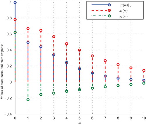
Figure 2. Weighted state norm and state response with a static output-feedback controller ($x_1(0)=0.62$, $x_2(0)=0.78$).

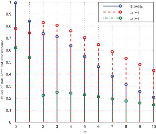
Table 1. Controller gains

$m$	$M(m)$	$K(m)$
0	$[-4.3455,-3.3795]$	$-1.2643$
1	$[-3.7204,-3.2416]$	$-3.5902$
2	$[-3.995,-3.1121]$	$-3.8898$
3	$[-4.1064,-3.0608]$	$-3.9896$
4	$[-4.1568,-3.0209]$	$-4.0395$
5	$[-4.1832,-2.9812]$	$-4.0695$
6	$[-4.1985,-2.9251]$	$-4.0895$
7	$[-4.2045,-2.8302]$	$-4.1037$
8	$[-4.1985,-2.6483]$	$-4.1144$
9	$[-4.1711,-2.2971]$	$-4.1228$

5. Conclusion

The positivity, finite-time stability and static output-feedback control for time-varying discrete-time linear system have been investigated in this work. Finite-time stability for positive linear time-varying discrete-time systems has been defined. For controller design, a necessary and sufficient condition guaranteeing the finite-time stability and positivity of the closed-loop system has been obtained at first. Two conditions that are equivalent to provide finite-time stability have been given such that the controller is decoupled from the finite-time matrix variable. Then an iterative algorithm has been developed for designing the controller such that the system can be finite-time stable with positivity. The theoretical results and algorithm have been verified by an illustrative example.

correction

This article has been republished with minor changes. These changes do not impact the academic content of the article.

Additional information

Funding

The authors received no direct funding for this research.

Notes on contributors

Jason J. R. Liu

All the authors of this work are or were members of Control and Automation Lab (CAL) of the University of Hong Kong with Prof. James Lam as the leader. The research areas of CAL include, but not limited to, model reduction, robust synthesis, delay systems, singular systems, stochastic systems, multidimensional systems, positive systems, networked control systems and vibration control.

James Lam

All the authors of this work are or were members of Control and Automation Lab (CAL) of the University of Hong Kong with Prof. James Lam as the leader. The research areas of CAL include, but not limited to, model reduction, robust synthesis, delay systems, singular systems, stochastic systems, multidimensional systems, positive systems, networked control systems and vibration control.

Xin Gong

All the authors of this work are or were members of Control and Automation Lab (CAL) of the University of Hong Kong with Prof. James Lam as the leader. The research areas of CAL include, but not limited to, model reduction, robust synthesis, delay systems, singular systems, stochastic systems, multidimensional systems, positive systems, networked control systems and vibration control.

Xiaochen Xie

All the authors of this work are or were members of Control and Automation Lab (CAL) of the University of Hong Kong with Prof. James Lam as the leader. The research areas of CAL include, but not limited to, model reduction, robust synthesis, delay systems, singular systems, stochastic systems, multidimensional systems, positive systems, networked control systems and vibration control.

Yukang Cui

All the authors of this work are or were members of Control and Automation Lab (CAL) of the University of Hong Kong with Prof. James Lam as the leader. The research areas of CAL include, but not limited to, model reduction, robust synthesis, delay systems, singular systems, stochastic systems, multidimensional systems, positive systems, networked control systems and vibration control.

References

- Amato, F., Ambrosino, R., Ariola, M., & Cosentino, C. (2009). Finite-time stability of linear time-varying systems with jumps. Automatica, 45(5), 1354–10. https://doi.org/10.1016/j.automatica.2008.12.016
- Amato, F., Ambrosino, R., Ariola, M., Cosentino, C., & De Tommasi, G. (2014). Finite-time Stability and Control (Vol. 453). Springer.
- Amato, F., & Ariola, M. (2005). Finite-time control of discrete-time linear systems. IEEE Transactions on Automatic Control, 50(5), 724–729. https://doi.org/10.1109/TAC.2005.847042
- Amato, F., Ariola, M., Carbone, M., & Cosentino, C. (2005). Finite-time output feedback control of discrete-time systems. Proceedings of 16th Triennial IFAC World Congress, 38(1), 514–519. https://doi.org/10.3182/20050703-6-CZ-1902.00486
- Amato, F., Ariola, M., & Cosentino, C. (2010a). Finite-time control of discrete-time linear systems: Analysis and design conditions. Automatica, 46(5), 919–924. https://doi.org/10.1016/j.automatica.2010.02.008
- Amato, F., Ariola, M., & Cosentino, C. (2010b). Finite-time stability of linear time-varying systems: Analysis and controller design. IEEE Transactions on Automatic Control, 55(4), 1003–1008. https://doi.org/10.1109/TAC.2010.2041680
- Bapat, R. B., Raghavan, T., & Bapat, R. B. (1997). Non-negative Matrices and Applications (Vol. 64). Cambridge University Press.
- Dorato, P. (1961). Short-time stability in linear time-varying systems (Technical Report). Polytechnic Inst of Brookklyn NY Microwave Research Institute.
- Ebihara, Y., Zhu, B., & Lam, J. (2020). The Lq/Lp Hankel norms of positive systems. IEEE Control Systems Letters, 4(2), 462–467. https://doi.org/10.1109/LCSYS.2019.2952622
- Farina, L., & Rinaldi, S. (2011). Positive Linear Systems: Theory and Applications (Vol. 50). John Wiley & Sons.
- Haddad, W. M., Chellaboina, V., & Hui, Q. (2010). Non-negative and Compartmental Dynamical Systems. Princeton University Press.
- Hong, M. T. (2019). An optimization approach to static output-feedback control of lti positive systems with delayed measurements. Journal of the Franklin Institute, 356(10), 5087–5103. https://doi.org/10.1016/j.jfranklin.2019.05.001
- Kaczorek, T. (2015). Positivity and stability of time-varying discrete-time linear systems. Proceedings of Asian conference on intelligent information and database systems (pp. 295–303). Springer.
- Kamenkov, G. (1953). On stability of motion over a finite interval of time. Journal of Applied Mathematics and Mechanics, 17(2), 529–540. https://doi.org/10.1016/0021-8928(68)90027-0
- Lebedev, A. (1954). The problem of stability in a finite interval of time. Journal of Applied Mathematics and Mechanics, 18(1), 75–94.
- Liu, J. J. R., Lam, J., & Shu, Z. (2020). Positivity-preserving consensus of homogeneous multiagent systems. IEEE Transactions on Automatic Control, 65(6), 2724–2729. https://doi.org/10.1109/TAC.2019.2946205
- Liu, L.-J., Karimi, H. R., & Zhao, X. (2018). New approaches to positive observer design for discrete-time positive linear systems. Journal of the Franklin Institute, 355(10), 4336–4350. https://doi.org/10.1016/j.jfranklin.2018.04.015
- Mirabdollahi, S., & Haeri, M. (2019). Multi-agent system finite-time consensus control in the presence of disturbance and input saturation by using of adaptive terminal sliding mode method. Cogent Engineering, 6(1), 1698689. https://doi.org/10.1080/23311916.2019.1698689
- Ogura, M., Kishida, M., & Lam, J. (2019). Geometric programming for optimal positive linear systems. IEEE Transactions on Automatic Control. https://doi.org/10.1109/TAC.2019.2960697
- Phat, V. N., & Sau, N. H. (2018). Exponential stabilisation of positive singular linear discrete-time delay systems with bounded control. IET Control Theory & Applications, 13(7), 905–911. https://doi.org/10.1049/iet-cta.2018.5150
- Ren, H., Zong, G., & Li, T. (2018). Event-triggered finite-time control for networked switched linear systems with asynchronous switching. IEEE Transactions on Systems, Man, and Cybernetics: Systems, 48(11), 1874–1884. https://doi.org/10.1109/TSMC.2017.2789186
- Shang, H., Qi, W., & Zong, G. (2019). Finite-time asynchronous control for positive discrete-time markovian jump systems. IET Control Theory & Applications, 13(7), 935–942. https://doi.org/10.1049/iet-cta.2018.5268
- Song, J., Niu, Y., & Wang, S. (2017). Robust finite-time dissipative control subject to randomly occurring uncertainties and stochastic fading measurements. Journal of the Franklin Institute, 354(9), 3706–3723. https://doi.org/10.1016/j.jfranklin.2016.07.020
- Song, J., Niu, Y., & Zou, Y. (2016). Finite-time sliding mode control synthesis under explicit output constraint. Automatica, 65, 111–114. https://doi.org/10.1016/j.automatica.2015.11.037
- Wang, C., & Zhao, Y. (2019). Performance analysis and control of fractional-order positive systems. IET Control Theory & Applications, 13(7), 928–934. https://doi.org/10.1049/iet-cta.2018.5225
- Wang, P., & Zhao, J. (2020). Stability and guaranteed cost analysis of switched positive systems with mode-dependent dwell time and sampling. IET Control Theory & Applications, 14(3), 378–385. https://doi.org/10.1049/iet-cta.2019.0466
- Wu, H., Lam, J., & Su, H. (2019). Global consensus of positive edge system with sector input nonlinearities. IEEE Transactions on Systems, Man, and Cybernetics: Systems, 1–10. https://doi.org/10.1109/TSMC.2019.2931411
- Xie, X., Lam, J., & Li, P. (2017). Finite-time H∞ control of periodic piecewise linear systems. International Journal of Systems Science, 48(11), 2333–2344. https://doi.org/10.1080/00207721.2017.1316884
- Xue, W., & Li, K. (2015). Positive finite-time stabilization for discrete-time linear systems. Journal of Dynamic Systems, Measurement, and Control, 137(1), 014502. https://doi.org/10.1115/1.4028141
- Yang, H., Zhang, J., Jia, X., & Li, S. (2019). Non-fragile control of positive Markovian jump systems. Journal of the Franklin Institute, 356(5), 2742–2758. https://doi.org/10.1016/j.jfranklin.2019.02.008
- Zhu, S., Wang, B., & Zhang, C. (2017). Delay-dependent stochastic finite-time l1 -gain filtering for discrete-time positive Markov jump linear systems with time-delay. Journal of the Franklin Institute, 354(15), 6894–6913. https://doi.org/10.1016/j.jfranklin.2017.07.008
- Zong, G., Yang, D., Hou, L., & Wang, Q. (2013). Robust finite-time H∞ control for Markovian jump systems with partially known transition probabilities. Journal of the Franklin Institute, 350(6), 1562–1578. https://doi.org/10.1016/j.jfranklin.2013.04.003